SU(5)+ADJOINT HIGGS AT FINITE TEMPERATURE

I present a three-dimensional effective theory that describes the high-temperature equilibrium behavior of the SU(5) theory accurately, but is much easier to study using non-perturbative methods than the original four-dimensional one. The effective theory is obtained by perturbatively integrating out the super-heavy Matsubara modes as well as the heavy temporal component of the gauge field. Regardless of the particle spectrum of the original theory, the resulting three-dimensional theory contains only a gauge field and an adjoint Higgs field. The phase diagram of the theory is analysed perturbatively and it is shown to have a cellular structure in three-dimensional parameter space.

1 GUT transition

If the Standard Model is a effective low-energy theory of a grand unified theory, there may have been a GUT phase transition in the very early universe. It would have taken place when the temperature was $T\sim 10^{16}$ GeV and would have had important cosmological effects.

Topological defects are necessarily created in the transition. Depending on the precise form of the GUT, these may be strings, domain walls or textures, but in any case there are monopoles, since the fundamental group of the Standard Model gauge group SU(3)$\times$SU(2)$\times$U(1) is non-trivial. The defects are important, since they can give rise to structure formation in the universe. However, the formation of a high density of monopoles is in conflict with standard cosmology and with observations. This monopole problem can be solved if the universe enters an exponentially expanding, inflationary phase in this or in some other transition taking place soon after the GUT one. Since GUTs do not conserve baryon number it is also possible that baryon asymmetry was generated. $B+L$ would be washed out later in the electroweak transition, but $B-L$ would remain. However, the simplest GUT candidate SU(5) does not violate $B-L$.

2 SU(5) dimensional reduction

From the low-energy physics one cannot deduce the form of the GUT. To understand the consequences of the transition even on a qualitative level, one still needs to have some concrete theory with which to make the calculations. The obvious choice is the SU(5) model suggested by Georgi and Glashow$\!{}^{{\bf?}}$, since it has the simplest structure. Furthermore, we drop the fermion fields and the fundamental Higgs field, since they are inessential when describing the transition. Thus we have a theory with a gauge field $A_{\mu}$ and an adjoint Higgs field $\Phi$. The Lagrangian of the theory is

$${\cal L}_{M}=-\frac{1}{2}{\rm Tr}F_{\mu\nu}F^{\mu\nu}+{\rm Tr}D_{\mu}\Phi D^{\mu}\Phi-m^{2}{\rm Tr}\Phi^{2}-\lambda_{1}({\rm Tr}\Phi^{2})^{2}-\lambda_{2}{\rm Tr}\Phi^{4},$$ (1)

where $D_{\mu}\Phi=\partial_{\mu}\Phi+ig[A_{\mu},\Phi].$

In the perturbative broken phase the system can be parametrized by the vector mass $M$, the SU(3) octet scalar mass $m_{8}$, the neutral scalar mass $m_{1}$ and the gauge coupling constant that is chosen to have the value $g\approx 0.39$ given by the running of the Standard Model coupling constants.

Since a gauge symmetry cannot be broken, the only non-perturbatively meaningful operators are gauge-invariant. Thus the simplest local fields are

$${\rm Tr}\Phi^{n},\quad{\rm Tr}F_{\mu\nu}\Phi^{(n-1)},\mbox{ where }2\leq n\leq 5.$$ (2)

In the broken phase these can be identified with the photon and a neutral scalar. In the symmetric phase all fields are composite.

To investigate the transition we start from the standard finite-temperature formalism. The temporal dimension gets replaced by a compact one, which can be integrated out perturbatively in dimensional reduction$\!{}^{{\bf?}}$. No infrared divergences appear in this calculation since they arise from the static modes which are still present in the effective three-dimensional theory. The calculation is performed by comparing one- and two-loop Green’s functions in the 4d finite-T theory and the 3d effective theory. Since the temporal component of the gauge field $A_{0}$ gets a heavy Debye mass, it can be also be integrated out. Thus we are left with an effective theory of the form

$${\cal L}=\frac{1}{2}{\rm Tr}F_{ij}F_{ij}+{\rm Tr}(D_{i}\overline{\Phi})^{2}+\overline{m}^{2}{\rm Tr}\overline{\Phi}^{2}+\overline{\lambda}_{1}({\rm Tr}\overline{\Phi}^{2})^{2}+\overline{\lambda}_{2}{\rm Tr}\overline{\Phi}^{4}.$$ (3)

The details of the calculation and the relations between 4d and 3d parameters are given in Ref.$\!{}^{{\bf?}}$.

The form of the effective potential does not depend on the original particle spectrum. All the fermions are integrated out since they have no static modes and all the other scalars get an effective mass from the thermal corrections and are integrated out along with the $A_{0}$ field. Thus their only contribution is to change the relation between the 3d and 4d parameters. This justifies the assumption that they are inessential in this context.

3 Effective theory

The parameters of the effective theory (3) are dimensionful. Thus we can use one of them to fix the scale and parametrize the theory by three dimensionless numbers

$$y=\frac{\overline{m}^{2}(\overline{g}^{2})}{\overline{g}^{4}},\quad x_{1}=\frac{\overline{\lambda}_{1}}{\overline{g}^{2}},\quad x_{2}=\frac{\overline{\lambda}_{2}}{\overline{g}^{2}}.$$ (4)

The theory is superrenormalizable and only the mass parameter must be renormalized. Its running can be calculated exactly in a two-loop perturbative calculation.

The relation between 4d and 3d parameters given in terms of the perturbative broken phase masses is

$$x_{1} \approx 0.21\frac{m_{1}^{2}}{M^{2}}-0.59\frac{m_{8}^{2}}{M^{2}}-0.012,\quad x_{2}\approx 2.52\frac{m_{8}^{2}}{M^{2}}-0.020,$$

$$y \approx 6.80+6.08\frac{m_{8}^{2}}{M^{2}}-1.45\frac{m_{8}^{4}}{M^{4}}+3.95\frac{m_{1}^{2}}{M^{2}}-0.038\frac{m_{1}^{4}}{M^{4}}$$ (5)

$$-0.12\frac{m_{8}^{2}m_{1}^{2}}{M^{4}}-21.9\frac{m_{1}^{2}}{T^{2}},$$

where the logarithmic divergence on the temperature is neglected. Thus, as temperature decreases, $x_{1}$ and $x_{2}$ stay constant and $y$ decreases. Thus $y$ can be interpreted as a measure of temperature.

The effective theory can be analysed in perturbation theory. There are three different phases,

$$\langle\Phi\rangle=0,\quad\langle\Phi\rangle\sim{\rm Diag}(2,2,2,-3,-3),\quad\langle\Phi\rangle\sim{\rm Diag}(1,1,1,1,-4).$$ (6)

Calculation of the two-loop effective potential in both of the broken phases gives the phase diagram shown if Fig. 1. As the universe cools down, the SU(5) symmetry is broken down to either SU(4)$\times$U(1) or SU(3)$\times$SU(2)$\times$U(1). The transitions between the phases are always first-order ones in perturbation theory. However, lattice simulations on analogous, but simpler models$\!{}^{{\bf?}}$ suggest that at large values of $x_{1}$ and $x_{2}$ there is a crossover instead of a transition. This is possible since there is no symmetry breakdown connected to this transition.

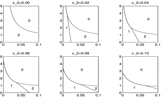
Figure 1: Cross-sections of the perturbative phase diagram of the effective theory at various values of $x_{2}$. Horizontal and vertical axes corresponds to $x_{1}$ and $y$, respectively. 0=symmetric phase, 1=SU(3)$\times$SU(2)$\times$U(1), 2=SU(4)$\times$U(1).

A numerical simulation would be the most reliable way to investigate the transition. On a lattice the theory (3) obtains the form

$${\cal L}_{\rm latt} = \frac{1}{a^{4}g^{2}}\sum_{i,j}{\rm Tr}\left[{\bf 1}-P_{ij}(x)\right]$$ (7)

$$+\frac{2}{a^{2}}\sum_{i}\left[{\rm Tr}\Phi(x)^{2}-{\rm Tr}\Phi(x)U_{i}(x)\Phi(x+i)U_{i}^{-1}(x)\right]$$

$$+m^{2}{\rm Tr}\Phi^{2}+\lambda_{1}({\rm Tr}\Phi^{2})^{2}+\lambda_{2}{\rm Tr}\Phi^{4},$$

where $a$ is the lattice spacing. Owing to superrenormalizability the lattice parameters can be related to the continuum ones with a two-loop calculation in lattice perturbation theory. In practice this means calculating the two-loop effective potential. This has been performed explicitly in Ref.$\!{}^{{\bf?}}$. This gives a connection between the 4d continuum and 3d lattice parameters.

At present there are no lattice simulations of this model. They would be interesting also independently of the original GUT model, since SU(5) has much more structure than e.g. SU(2). Thus its phase transition could exhibit some interesting non-perturbative phenomena.

4 Conclusions

We constructed explicitly a three-dimensional purely bosonic effective theory that describes the equilibrium behavior of the SU(5) GUT near the transition. We also analysed it perturbatively and found its phase diagram. However, lattice simulation is needed to get reliable information. To this end we calculated the relation between lattice and continuum parameters. However, no simulations have yet been made.

In analogous but simpler models the transition is a crossover for some parameter values. If the same is true here, it would change the picture of the GUT transition. If there is only a crossover, the cosmological consequences are much smaller than in the first-order case, since the system can stay near the equilibrium. In practice this rules out both baryogenesis and inflation in this transition, but does not cure the monopole problem, since the monopoles formed by thermal fluctuations still fall out of equilibrium and their density remains far too high.

References

References

- [1] H. Georgi and S.L. Glashow, Phys. Rev. Lett. 32, 438 (1974).
- [2] M. Laine, these proceedings; K. Kajantie, M. Laine, K. Rummukainen and M. Shaposhnikov, Nucl. Phys. B 458, 90 (1996) and references therein.
- [3] A. Rajantie, hep-ph/9702255, to be published in Nucl. Phys. B.
- [4] A. Hart, O. Philipsen, J.D. Stack and M. Teper, Phys. Lett. B 396, 217 (1997); K. Kajantie, M. Laine, K. Rummukainen and M. Shaposhnikov, hep-ph/9704416.
- [5] M. Laine and A. Rajantie, hep-lat/9705003.