hep-ph/9708350 PITHA 97/29

Next-to-Leading Order QCD Corrections
and Massive Quarks in $e^{+}e^{-}\to 3$ Jets

Arnd Brandenburg^, and Peter Uwer

Institut für Theoretische Physik, RWTH Aachen, D-52056 Aachen, Germany

Abstract:
We present in detail a calculation of the next-to-leading order QCD corrections to the process $e^{+}e^{-}\to 3$ jets with massive quarks. To isolate the soft and collinear divergencies of the four parton matrix elements, we modify the phase space slicing method to account for masses. Our computation allows for the prediction of oriented three jet events involving heavy quarks, both on and off the Z resonance, and of any event shape variable which is dominated by three jet configurations. We show next-to-leading order results for the three jet fraction, the differential two jet rate, and for the thrust distribution at various c.m. energies.

PACS numbers: 12.38.Bx, 13.87.Ce, 14.65.Fy

1 Introduction

High energy $e^{+}e^{-}$ annihilation experiments have proven to be a particularly clean testing ground for quantum chromodynamics (QCD), the theory of strong interactions. One of the key predictions of QCD has been the occurence of jets of hadrons in high energy reactions [1, 2]. Quantitatively, the observed hadronic events can be classified according to the number of jets. The most commonly used definitions of jets in $e^{+}e^{-}$ annihilation are based on iterative jet clustering algorithms. One begins with a set of final-state particles, and considers for each iteration the pair $\{i,j\}$ with the smallest value of a dimensionless measure $y_{ij}$. If this $y_{ij}$ is smaller than a preset cutoff $y_{cut}$, the pair is clustered into a single pseudoparticle according to a recombination rule. The procedure is repeated until $y_{ij}>y_{cut}$ for all pairs of (pseudo-)particles, at which point the remaining objects are called jets. In the perturbative calculation, the quantity $y_{ij}$ is constructed from the parton momenta.

There exist a number of jet observables that are well defined in QCD, and which can be calculated perturbatively as an expansion in the strong coupling $\alpha_{s}$. It is also possible to define a variety of quantities (so-called event shape variables) that depend on the final state structure and do not need the above concept of a jet. One of the well-known event shape variables is thrust [3]. The only requirement for such quantities is that they are infrared safe, i.e. they neither distinguish between a final state with one particle being soft and a final state where this particle is absent, nor between a final state with two collinear partons and a final state where these two collinear partons are clustered into a single hard pseudoparticle. Infrared safe quantities that are dominated by three jet configurations, and the three jet differential cross section (defined by the jet algorithm described above) are of interest, in particular because these quantities are in leading order (LO) proportional to $\alpha_{s}$. The next-to-leading order (NLO) QCD corrections to the production of three partons were computed more than fifteen years ago [4, 5, 6, 7] for massless quarks. Subsequently, these results have been implemented in numerical programs [8]–[13] and widely used for tests of QCD with jet physics. Also, a complete calculation for oriented three jet events with massless quarks was performed in [14, 15].

To date huge samples of jet events produced at the $Z$ resonance have been collected both at LEP and SLC. From these data large numbers of jet events involving $b$ quarks can be isolated with high purity using vertex detectors. While the mass of the $b$ quark can be neglected to good approximation in the computation of the total $b\bar{b}$ production rate at the $Z$ peak, the n-jet cross sections depend, apart from the c.m. energy $\sqrt{s}$, on an extra scale, namely the jet resolution parameter $y_{cut}$. For small $y_{cut}$ effects due to quark masses can be enhanced. It is therefore desirable for precision tests of QCD to use NLO matrix elements that include the full quark mass dependence. One can then also try to extract the mass of the $b$ quark from three jet rates involving $b$ quarks at the $Z$ peak, as suggested in [16], elaborated in [17], [18], and experimentally pursued by the DELPHI collaboration [19]. Further applications include precision tests of the asymptotic freedom property of QCD by means of three jet rates and event shape variables measured at various center-of-mass energies, also far below the $Z$ resonance [20]. For theoretical predictions concerning the production of top quark pairs at a future $e^{+}e^{-}$ collider, the inclusion of the full mass dependence is of course mandatory.

The three, four, and five jet rates involving massive quarks have been computed to leading order in $\alpha_{s}$ already some time ago [21, 22]. In reference [23], the NLO corrections to the production of a heavy quark pair plus a hard photon are given. Recently, results for the decay rate of the $Z$ boson and the $e^{+}e^{-}$ annihilation cross section at the $Z$ peak into three jets including mass effects at NLO have been reported [17], [24], [18]. Further, momentum correlations in $Z\to b\bar{b}X$ at NLO have been studied [25].

We have computed the complete differential distributions for $e^{+}e^{-}$ annihilation into three and four partons via a virtual photon or $Z$ boson at order $\alpha_{s}^{2}$, including the full quark mass dependence. This allows for order $\alpha_{s}^{2}$ predictions of oriented three jet events, and of any quantity that gets contributions only from three and four jet configurations. In this article, we would like to discuss this calculation in detail. We start in section 2 with an overview of the calculation. Section 3 contains a general kinematical analysis and the LO results for $e^{+}e^{-}\to 3$ jets including mass effects. The virtual corrections are discussed in section 4. They contain singularities that cancel against real soft and collinear contributions from four parton final states. To isolate the latter contributions, a modification of the phase space slicing method incorporating massive partons is developed in section 5. In section 6 we show numerical results. In particular, we compare for some observables the massive with the massless result. We summarize our results in section 7. An Appendix contains the analytical result for the virtual corrections to the three parton production rate.

2 Outline of the calculation

The calculation of an arbitrary quantity dominated by three jet configurations and involving a massive quark-antiquark pair to order $\alpha_{s}^{2}$ proceeds as follows:

We first have to compute the fully differential cross section for the partonic reaction

$$e^{+}e^{-}\to\gamma^{\ast},Z^{\ast}\to Q\bar{Q}g$$ (2.1)

at leading and next-to-leading order in $\alpha_{s}$. Here $Q$ denotes a massive quark and $g$ a gluon.

At leading order, the parton momenta can be identified with the jet momenta. If the identity of the particles making up the jets is known, we have for the differential three jet cross section

$$d\sigma_{1}(e^{+}e^{-}\to 3\ {\rm jets})=\Theta(y_{Q\bar{Q}}-y_{cut})\Theta(y_{Qg}-y_{cut})\Theta(y_{\bar{Q}g}-y_{cut})d\sigma_{1}(e^{+}e^{-}\to Q\bar{Q}g),$$ (2.2)

where the lower index 1 means the result in order $\alpha_{s}^{1}$, $\Theta$ is the Heaviside step function, $y_{cut}$ is the jet resolution parameter and $y_{ij}\in\{y_{Q\bar{Q}},y_{Qg},y_{\bar{Q}g}\}$ is determined by the experimental jet definition. For example

$$y_{ij}\ = \ \frac{2E_{i}E_{j}}{s}(1-\cos\theta_{ij})\ \ \ \ \ {\mbox{ for the JADE algorithm \cite[cite]{[\@@bibref{}{Ba86}{}{}]}}},$$

$$y_{ij}\ = \ \frac{2\ {\mbox{min}}\{E_{i}^{2},E_{j}^{2}\}}{s}(1-\cos\theta_{ij})\ \ \ \ \ {\mbox{ for the Durham algorithm \cite[cite]{[\@@bibref{}{Br90}{}{}]}}},$$ (2.3)

where $\theta_{ij}$ is the angle between jet $i$ and $j$ in the c.m. system. At higher order and in the experimental analysis, these definitions are supplemented by a recombination rule to form a pseudoparticle $k$ from a clustered pair $\{i,j\}$. For the above algorithms, one simply adds the four-momenta, $p_{k}=p_{i}+p_{j}$. (For a detailed discussion of these and other jet algorithms, see also [31].) If the particle content of one or more jets is not known, the LO calculation of a three-jet quantity from $d\sigma_{1}(e^{+}e^{-}\to Q\bar{Q}g)$ may involve an averaging over the different ways of assigning jet momenta to parton momenta.

The one-loop integrals, which appear in the NLO amplitude for (2.1), contain ultraviolet (UV) and infrared (soft and collinear) (IR) singularities. In the framework of dimensional regularization in $d=4-2\epsilon$ space-time dimensions, these singularities appear as poles in $\epsilon$. The UV singularities are removed by renormalization. Details will be given in section 4.

After renormalization, the virtual corrections to the differential cross section for (2.1) still contain IR singularities. These have to be cancelled by the singularities that are obtained upon phase space integration of the squared tree amplitudes for the production of four partons. The relevant processes are

$$e^{+}e^{-}\to\gamma^{\ast},Z^{\ast}\to Q\bar{Q}gg,$$ (2.4)

$$e^{+}e^{-}\to\gamma^{\ast},Z^{\ast}\to Q\bar{Q}q\bar{q},$$

$$e^{+}e^{-}\to\gamma^{\ast},Z^{\ast}\to Q\bar{Q}Q\bar{Q},$$

where $q$ denotes a light (massless) quark. The first two reactions of (2.4) give singular contributions in the three jet region when a parton becomes soft and/or two partons become collinear. The cancellation of the singularities has of course to be performed analytically. To this end, the soft and collinear poles of the relevant four parton matrix elements have to be explicitly isolated. We do this by modifying the so-called phase space slicing method [10] to account for masses. (For alternative methods, see, e.g., [11, 12, 13] and references therein.)

The idea of the phase space slicing method is to introduce an unphysical parameter $s_{min}$, which is much smaller than all relevant physical scales of the problem, e.g. $s_{min}\ll sy_{cut}$ for jet cross sections defined by the jet resolution $y_{cut}$. The parameter $s_{min}$ splits the four parton phase space into a region where all partons are “resolved” and a region where at least one parton is soft and/or two partons are collinear. In the massless case, a convenient definition of the resolved region is given by the requirement $s_{ij}>s_{min}$ for all invariants $s_{ij}=(p_{i}+p_{j})^{2}$. We will modify this definition to account for masses, see section 5, but still will use the terminology “resolved” and “unresolved” partons. In the regions with unresolved partons, soft and collinear approximations of the matrix elements, which hold exactly in the limit $s_{min}\to 0$, are used. The necessary integrations over the soft and collinear regions of phase space can then be carried out analytically in $d$ dimensions. One can thus isolate all the poles in $\epsilon$ and perform the cancellation of the IR singularities between real and virtual contributions, after which one takes the limit $\epsilon\to 0$ (cf. eq. (5)). The result is a finite differential cross section $d\sigma_{2}^{R}(e^{+}e^{-}\to Q\bar{Q}g)$ at order $\alpha_{s}^{2}$ for three resolved partons, which depends on $s_{min}$. Its contribution to a given three-jet quantity is specified by the experimental jet definition, which may involve an energy ordering, a tagging prescription, etc.

The contribution to a three jet quantity or to an event shape variable of the resolved part of the four parton cross sections $d\sigma_{2}^{R}(e^{+}e^{-}\to 4\ {\rm partons})$ is finite by itself and may be evaluated in $d=4$ dimensions, which greatly simplifies the algebra. Its contribution to three jet configurations also depends on $s_{min}$ and is obtained by recombining the four resolved partons into three jets according to some recombination scheme and by projecting the four parton phase space onto the experimentally specified three jet phase space.

Since the parameter $s_{min}$ is introduced in the theoretical calculation for technical reasons only and unrelated to any physical quantity, the sum of all contributions to any three jet observable must not depend on $s_{min}$. In the soft and collinear approximations one neglects terms which vanish as $s_{min}\to 0$. This limit can be carried out numerically. Since the individual contributions depend logarithmically on $s_{min}$, it is a nontrivial test of the calculation to demonstrate that the sum of resolved and unresolved contributions becomes independent of $s_{min}$ for small values of this parameter. Moreover, in order to avoid large numerical cancellations, one should determine the largest value of $s_{min}$ which has this property.

Schematically, we have for the differential three jet cross section involving massive quarks at order $\alpha_{s}^{2}$:

$$d\sigma_{2}(e^{+}e^{-}\to 3\ {\rm jets})\ = \ {\bf{\Theta}}\bigg{\{}d\sigma_{2}^{R}(e^{+}e^{-}\to Q\bar{Q}g)$$

$$+ \ \int\bigg{[}d\sigma_{2}^{R}(e^{+}e^{-}\to Q\bar{Q}gg)+d\sigma_{2}^{R}(e^{+}e^{-}\to Q\bar{Q}q\bar{q})$$

$$+ \ d\sigma_{2}^{R}(e^{+}e^{-}\to Q\bar{Q}Q\bar{Q})\bigg{]}\bigg{\}},$$ (2.5)

where ${\bf{\Theta}}$ contains the experimental jet definition, and the integration symbol contains the procedure of recombining resolved partons into jets and of projecting the four parton phase space onto the three jet phase space. Eq. (2) is schematic in the sense that the exact relation between a given three jet quantity and the parton cross sections depends on the experimental knowledge about the jets, as already mentioned above.

It should be emphasized that the notion of resolved/unresolved partons is unrelated to the physical jet resolution criterium or to any other relevant physical scale. In particular, we will use the freedom in defining the soft and collinear regions of phase space to simplify the necessary analytic integrations in $d$ dimensions. Explicit expressions for the resolved cross sections entering (2) will be derived in section 5.

The fully differential cross section for the production of two jets with massive quarks is known to order $\alpha_{s}$ already for some time [26]. For order $\alpha_{s}^{2}$ calculations of quantities that also get contributions from two jet configurations, the two loop amplitude for $e^{+}e^{-}\to Q\bar{Q}$ is needed. Results for the total cross section for $e^{+}e^{-}\to$ hadrons to order $\alpha_{s}^{2}$ with mass corrections are reviewed in [27]. (For recent results see also [28].) Since

$$\sigma(e^{+}e^{-}\to{\mbox{hadrons}}) = \sigma(e^{+}e^{-}\to{\mbox{2 jets}})+\sigma(e^{+}e^{-}\to{\mbox{3 jets}})$$ (2.6)

$$+ \sigma(e^{+}e^{-}\to{\mbox{4 jets}})+O(\alpha_{s}^{3}),$$

one can now also calculate the two jet cross section to this order, but not yet arbitrary differential distributions.

3 Kinematics and leading order results

In this section we review some of the basic kinematics relevant for the process

$$e^{+}(p_{+})e^{-}(p_{-})\rightarrow Z^{\ast},\gamma^{\ast}\rightarrow Q(k_{1})\bar{Q}(k_{2})g(k_{3})$$ (3.1)

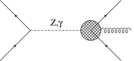
Figure 1: Amplitude for the process $e^{+}(p_{+})e^{-}(p_{-})\rightarrow Z^{\ast},\gamma^{\ast}\rightarrow Q(k_{1})\bar{Q}(k_{2})g(k_{3})$

and give the leading order results for the fully differential cross section for (3.1). The amplitude ${\cal T}$ for the reaction (3.1) (see also Fig. 1) can be written, to order $\alpha_{s}^{3/2}$ and to leading order in the electroweak couplings in the general form:

$${\cal T} = \frac{4\pi\alpha}{s}\Big{\{}\,\chi(s)\,\bar{v}(p_{+})(g_{v}^{e}\gamma_{\mu}-g_{a}^{e}\gamma_{\mu}\gamma_{5})u(p_{-})\,(g_{v}^{Q}V^{\mu}-g_{a}^{Q}A^{\mu}-\sum_{i}g_{a}^{i}A_{i}^{\mu})$$ (3.2)

$$+ \bar{v}(p_{+})\gamma_{\mu}u(p_{-})(-Q_{Q}V^{\mu})\Big{\}}.$$

In (3.2), $s=(p_{+}+p_{-})^{2}$, $Q_{Q}$ denotes the electric charge of the quark in units of $e=\sqrt{4\pi\alpha}$, and $g_{v}^{f}$, $g_{a}^{f}$ are the vector- and the axial-vector couplings of a fermion of type $f$, i.e.

$$g_{v}^{f}=T_{3}^{f}-2\,Q_{f}\,\sin^{2}\vartheta_{W},\quad\mbox{and}\quad g_{a}^{e}=T_{3}^{f}.$$

In particular, $g_{v}^{e}=-\frac{1}{2}+2\sin^{2}\vartheta_{W}$, $g_{a}^{e}=-\frac{1}{2}$ for an electron or $g_{v}^{b}=-\frac{1}{2}+\frac{2}{3}\sin^{2}\vartheta_{W}$, $g_{a}^{b}=-\frac{1}{2}$ for a bottom quark, with $\vartheta_{W}$ denoting the weak mixing angle. The function $\chi(s)$ is given by

$$\chi(s)=\frac{1}{4\sin^{2}\vartheta_{W}\cos^{2}\vartheta_{W}}\,\frac{s}{s-m_{Z}^{2}+im_{Z}\Gamma_{Z}},$$ (3.3)

where $m_{Z}$ and $\Gamma_{Z}$ stand for the mass and the width of the Z-boson. We have defined in (3.2) the amplitudes $V^{\mu},\ A^{\mu}$, and $A^{\mu}_{i}$, which contain the information on the decay of the vector boson into the three final state partons. The contribution $A^{\mu}_{i}$ is generated at order $\alpha_{s}^{3/2}$ by a quark triangle loop [32]. The sum runs over the different quark flavors. Only quark doublets with a mass-splitting give a non-vanishing contribution. At higher order in $\alpha_{s}$ there are additional terms in eq. (3.2) of the form $V_{i}^{\mu}$, which are absent at order $\alpha_{s}^{3/2}$ due to a non-abelian generalization of Furry’s theorem. Such additional terms are also present in the scattering amplitude for the four parton final state $q\bar{q}Q\bar{Q}$ with light quarks at the initial vertex at lowest order in $\alpha_{s}$.

The squared amplitude $|{\cal T}|^{2}$ can be written to order $\alpha_{s}^{2}$ in the compact form:

$$|{\cal T}|^{2} = \frac{16\pi^{2}\alpha^{2}}{s^{2}}\Big{[}L^{PC\mu\nu}H^{PC}_{\mu\nu}+L^{PV\mu\nu}H^{PV}_{\mu\nu}\Big{]}.$$ (3.4)

We restrict ourselves here to the relevant case of longitudinal polarization of electrons and/or positrons and neglect the lepton masses. The lepton tensors $L^{PC\mu\nu}$ and $L^{PV\mu\nu}$ take the usual form:

$$L^{PC\mu\nu} = \frac{1}{4}\mbox{Tr}[p\!\!\!/_{+}\gamma^{\mu}p\!\!\!/_{-}\gamma^{\nu}]=p_{+}^{\mu}p_{-}^{\nu}+p_{+}^{\nu}p_{-}^{\mu}-g^{\mu\nu}p_{+}p_{-},$$

$$L^{PV\mu\nu} = \frac{1}{4}\mbox{Tr}[\gamma_{5}p\!\!\!/_{+}\gamma_{\mu}p\!\!\!/_{-}\gamma_{\nu}]=-i\varepsilon^{\mu\nu}_{\ \ \rho\sigma}p_{+}^{\rho}p_{-}^{\sigma},$$ (3.5)

where $\varepsilon_{0123}=+1$. The tensors $H^{PC(PV)}_{\mu\nu}$ (which we call “parton tensors”) may be written as follows:

$$H^{PC(PV)}_{\mu\nu}\ = \ g^{VV}_{PC(PV)}H^{VV}_{\mu\nu}+g^{AA}_{PC(PV)}H_{\mu\nu}^{AA}+g_{PC(PV)}^{VA_{+}}H_{\mu\nu}^{VA_{+}}+\sum_{i}g_{PC(PV)}^{AA^{i}}H_{\mu\nu}^{AA^{i}}$$ (3.6)

$$+ \sum_{i}g_{PC(PV)}^{VA_{+}^{i}}H_{\mu\nu}^{VA_{+}^{i}}+g_{PC(PV)}^{VA_{-}}H_{\mu\nu}^{VA_{-}}+\sum_{i}g_{PC(PV)}^{VA_{-}^{i}}H_{\mu\nu}^{VA_{-}^{i}}.$$

The coupling constants are given explicitly by

$$g_{PC(PV)}^{VV} = Q_{Q}^{2}\,f_{PC(PV)}^{\gamma\gamma}+2\,g_{v}^{Q}\,Q_{Q}\,\mbox{Re}\chi(s)\,f_{PC(PV)}^{\gamma Z}+g_{v}^{Q\,2}\,|\chi(s)|^{2}\,f_{PC(PV)}^{ZZ},$$

$$g_{PC(PV)}^{AA} = g_{a}^{Q\,2}|\chi(s)|^{2}f_{PC(PV)}^{ZZ},$$

$$g_{PC(PV)}^{VA_{+}} = -g_{a}^{Q}\,Q_{Q}\,\mbox{Re}\,\chi(s)\,f_{PC(PV)}^{\gamma Z}-g_{v}^{Q}\,g_{a}^{Q}\,|\chi(s)|^{2}f_{PC(PV)}^{ZZ},$$

$$g_{PC(PV)}^{AA_{i}} = g_{a}^{Q}\,g_{a}^{i}|\chi(s)|^{2}f_{PC(PV)}^{ZZ},$$

$$g_{PC(PV)}^{VA_{+}^{i}} = -g_{a}^{i}\,Q_{Q}\,\mbox{Re}\,\chi(s)\,f_{PC(PV)}^{\gamma Z}-g_{v}^{Q}\,g_{a}^{i}\,|\chi(s)|^{2}f_{PC(PV)}^{ZZ},$$

$$g_{PC(PV)}^{VA_{-}} = i\,g_{a}^{Q}\,Q_{Q}\,\mbox{Im}\chi(s)f_{PC(PV)}^{\gamma Z},$$

$$g_{PC(PV)}^{VA_{-}^{i}} = i\,g_{a}^{i}\,Q_{Q}\,\mbox{Im}\chi(s)f_{PC(PV)}^{\gamma Z},$$ (3.7)

where

$$f_{PC}^{\gamma\gamma} = 1-\lambda_{-}\lambda_{+},$$

$$f_{PC}^{\gamma Z} = -(1-\lambda_{-}\lambda_{+})g_{v}^{e}+(\lambda_{-}-\lambda_{+})g_{a}^{e},$$

$$f_{PC}^{ZZ} = (1-\lambda_{-}\lambda_{+})(g_{v}^{e2}+g_{a}^{e2})-2(\lambda_{-}-\lambda_{+})g_{v}^{e}g_{a}^{e},$$

$$f_{PV}^{\gamma\gamma} = \lambda_{-}-\lambda_{+},$$

$$f_{PV}^{\gamma Z} = (1-\lambda_{-}\lambda_{+})g_{a}^{e}-(\lambda_{-}-\lambda_{+})g_{v}^{e},$$

$$f_{PV}^{ZZ} = (\lambda_{-}-\lambda_{+})(g_{v}^{e\,2}+g_{a}^{e\,2})-2\,(1-\lambda_{-}\lambda_{+})g_{v}^{e}\,g_{a}^{e},$$ (3.8)

with $\lambda_{-}$ ($\lambda_{+}$) denoting the longitudinal polarization of the electron (positron) beam.

The parton tensors $H^{VV}_{\mu\nu},H^{AA}_{\mu\nu},\ldots$ are related to the amplitudes $V_{\mu},A_{\mu}$ and $A^{i}_{\mu}$ in the following way (we do not write down explicitly the sum over the polarizations of the final states):

$$H_{\mu\nu}^{VV} = V_{\mu}V_{\nu}^{\ast},$$

$$H_{\mu\nu}^{AA} = A_{\mu}A_{\nu}^{\ast},$$

$$H_{\mu\nu}^{VA_{\pm}} = V_{\mu}A_{\nu}^{\ast}\pm A_{\mu}V_{\nu}^{\ast},$$

$$H_{\mu\nu}^{VA^{i}_{\pm}} = V_{\mu}A_{i\nu}^{\ast}\pm A_{i\mu}V_{\nu}^{\ast},$$

$$H_{\mu\nu}^{AA^{i}} = A_{\mu}A_{\nu}^{i\ast}+A^{i}_{\mu}A_{\nu}^{\ast}.$$ (3.9)

In massless QCD chiral symmetry implies that $H^{VV}_{\mu\nu}=H^{AA}_{\mu\nu}$ and $H_{\mu\nu}^{VA_{-}}=0$. The tensors $H_{\mu\nu}^{VA_{-}}$ and $H_{\mu\nu}^{VA_{-}^{i}}$ multiply factors that are formally of higher order in the electroweak coupling. Their contributions to the differential cross section for (3.1) are negligibly small.

The parton tensors $H_{\mu\nu}$ entering (3.4) contain the complete information about the orientation of the partons in the final state with respect to the beam axis and about their energy distribution. Although the parton tensors are good for calculational purposes, we find it more convenient for the phenomenological application to switch to a slightly different notation, which we adopt from ref. [32]. We write the $e^{+}e^{-}\to\gamma^{\ast},Z^{\ast}\to Q\bar{Q}g$ fully differential cross section (in $d=4$ dimensions), with no transverse beam polarization, as follows:

$$\frac{d^{4}\sigma}{dx\,d\bar{x}\,d\cos\theta\,d\phi}\ = \ \frac{3}{4\pi}\frac{\alpha_{s}}{\pi}\sigma_{\rm pt}\Big{[}F_{1}(1+\cos^{2}\theta)+F_{2}(1-3\cos^{2}\theta)+F_{3}\cos\theta$$ (3.10)

$$+ F_{4}\sin 2\theta\cos\phi+F_{5}\sin^{2}\theta\cos 2\phi+F_{6}\sin\theta\cos\phi$$

$$+ F_{7}\sin 2\theta\sin\phi+F_{8}\sin^{2}\theta\sin 2\phi+F_{9}\sin\theta\sin\phi\Big{]}\ ,$$

where

$$\sigma_{\rm pt}\ =\ \sigma(e^{+}e^{-}\to\gamma^{*}\to\mu^{+}\mu^{-})\ =\ \frac{4\pi\alpha^{2}}{3s}\ .$$ (3.11)

In (3.10), $x=2kk_{1}/s$ and $\bar{x}=2kk_{2}/s$ are the scaled energies of the quark and antiquark in the $Z$ rest system, $\theta$ is the angle between the electron direction and the quark direction, and $\phi$ is the (signed) angle between the $e^{+}e^{-}Q$ plane and the $Q\bar{Q}g$ plane. The functions $F_{i}$ are easily obtained by contracting the parton tensors $H_{\mu\nu}$ with suitable tensors built from the final state momenta and $g_{\mu\nu}$.

The functions $F_{7},\ F_{8}$ and $F_{9}$ are generated by absorptive parts in the scattering amplitude, i.e. they are zero in tree-approximation. In addition they vanish for massless quarks at one loop order [33], [14]. For the nonvanishing LO functions $F_{i}$ we have:

$$F_{i}^{(0)} = g_{PC}^{VV}F_{i}^{(0),VV}+g_{PC}^{AA}F_{i}^{(0),AA}\ \ \ \ \ (i=1,2,4,5),$$

$$F_{j}^{(0)} = g_{PV}^{VA_{+}}F_{j}^{(0),VA_{+}}\ \ \ \ \ (j=3,6).$$ (3.12)

Using the abbreviations

$$z=\frac{m^{2}}{s},\ \ \ \ \ B=\frac{1}{(1-x)(1-\bar{x})},\ \ \ \ \ x_{g}=2-x-\bar{x},$$ (3.13)

where $m$ is the quark mass, we find:

$$F_{1}^{(0),VV} = B\bigg{\{}{x^{2}+\bar{x}^{2}\over 2}+z\left[-3(x+\bar{x})^{2}+8(x+\bar{x})+2x\bar{x}(1-x_{g})-6\right]B-2z^{2}x_{g}^{2}B\bigg{\}},$$

$$F_{1}^{(0),AA} = F_{1}^{(0),VV}+zB\bigg{\{}(x+\bar{x})^{2}-10(1-x_{g})+6zx_{g}^{2}B\bigg{\}},$$

$$F_{2}^{(0),VV} = \frac{1}{x^{2}-4z}\bigg{\{}1-x_{g}-z(-3x^{2}+\bar{x}^{2}-2x\bar{x}+2x-2\bar{x}+2)B$$

$$- 2z^{2}[2x^{3}-13x^{2}-5\bar{x}^{2}+2x\bar{x}(4x+3\bar{x}-11)+20x+12\bar{x}-8]B^{2}+8z^{3}x_{g}^{2}B^{2}\bigg{\}},$$

$$F_{2}^{(0),AA} = \frac{1-x_{g}}{x^{2}-4z}-\frac{z(1-\bar{x})[x^{3}-5x^{2}-3\bar{x}^{2}+x\bar{x}(2x+\bar{x}-8)+8x+6\bar{x}-2]-2z^{2}x_{g}^{2}}{(1-\bar{x})^{2}(x^{2}-4z)},$$

$$F_{3}^{(0),VA_{+}} = \frac{2B}{\sqrt{x^{2}-4z}}\bigg{\{}x^{3}+2\bar{x}^{2}+x\bar{x}(-\bar{x}+2)-2\bar{x}-2z[x^{3}-8x^{2}-4\bar{x}^{2}$$

$$+ x\bar{x}(6x+5\bar{x}-16)+12x+8\bar{x}-4]B+8z^{2}x_{g}^{2}B\bigg{\}},$$

$$F_{4}^{(0),VV} = \frac{B\sqrt{(1-x)(1-\bar{x})(1-x_{g})-zx_{g}^{2}}}{(x^{2}-4z)(\bar{x}^{2}-4z)}\bigg{\{}\bar{x}^{2}[2(1-x_{g})-x\bar{x}]$$

$$+ \frac{2z}{1-\bar{x}}[4\bar{x}^{2}+x\bar{x}(3\bar{x}^{2}+x\bar{x}-6\bar{x}+6)-4x-8\bar{x}+4$$

$$- 4z(\bar{x}^{3}+x^{2}-2\bar{x}^{2}+x\bar{x}(\bar{x}+3)-4x)-16z^{2}x_{g}]\bigg{\}},$$

$$F_{4}^{(0),AA} = F_{4}^{(0),VV}+\frac{4zB\sqrt{(1-x)(1-\bar{x})(1-x_{g})-zx_{g}^{2}}}{x^{2}-4z}\bigg{\{}x^{2}-2(1-x_{g})+x\bar{x}\bigg{\}}$$

$$F_{5}^{(0),VV} = F_{2}^{(0),VV}-2zB\bigg{\{}1-x_{g}-zx_{g}^{2}B\bigg{\}}$$

$$F_{5}^{(0),AA} = F_{2}^{(0),AA}-zx_{g}^{2}B,$$

$$F_{6}^{(0),VA_{+}} = 4B\sqrt{\frac{(1-x)(1-\bar{x})(1-x_{g})-zx_{g}^{2}}{x^{2}-4z}}\bigg{\{}\bar{x}-\frac{2zx_{g}}{1-\bar{x}}\bigg{\}}.$$ (3.14)

Our results agree with the results of [37] and reduce in the massless case to those given in [32]. The increase in algebraic complexity due to the non-neglection of the quark mass is quite substantial already at LO.

4 Virtual corrections

The calculation of the virtual corrections for reaction (3.1) is straightforward albeit tedious. Non-neglection of the quark mass leads to a considerable complication of the algebra. In this section we give details on this part of the calculation.

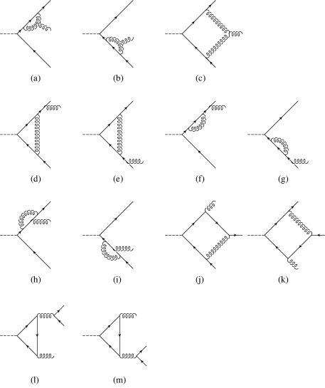
Figure 2: Loop diagrams.

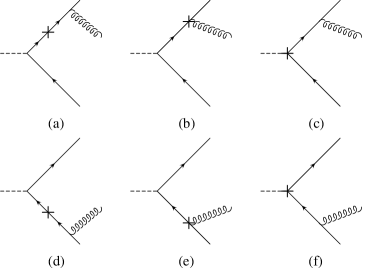
Figure 3: Counterterm diagrams.

We work in renormalized perturbation theory, i.e. start with a renormalized Lagrangian including counterterms to calculate the (truncated) renormalized Green function for reaction (3.1) in $d$ dimensions to order $\alpha_{s}^{3/2}$. The relevant one-loop diagrams are shown in figure 2, the counterterm diagrams are depicted in figure 3. The scattering amplitude,

$${\cal T}(e^{+}e^{-}\to Q\bar{Q}g)={\cal T}^{\scriptsize{\mbox{Born}}}(e^{+}e^{-}\to Q\bar{Q}g)+{\cal T}^{\scriptsize{\mbox{virtual}}}(e^{+}e^{-}\to Q\bar{Q}g)+O(\alpha_{s}^{2}),$$ (4.1)

follows from the renormalized truncated Green function by multiplication of UV finite wave function renormalization factors in accordance with the Lehmann-Symanzik-Zimmermann reduction formalism. Except for the quark mass renormalization, we work in the modified minimal subtraction (${\overline{\mbox{MS}}}$) scheme throughout. For the quark mass renormalization we consider both the on-shell scheme and the ${\overline{\mbox{MS}}}$ scheme. The relation between both schemes is given to order $\alpha_{s}$ by the well-known relation

$$m^{\rm pole}=m^{\scriptsize{\mbox{${\overline{\mbox{MS}}}$}}}(\mu)\left[1+\frac{\alpha_{s}(\mu)}{\pi}\left(\frac{4}{3}-2\ln\frac{m^{\scriptsize{\mbox{${\overline{\mbox{MS}}}$}}}(\mu)}{\mu}\right)\right],$$ (4.2)

where $\mu$ is the renormalization scale. It is somewhat more transparent to use the pole mass from the start and, if desired, switch to the ${\overline{\mbox{MS}}}$ scheme only at the very end of the calculation using (4.2). In an ab initio calculation with the ${\overline{\mbox{MS}}}$ mass one has to distinguish between the renormalized mass parameter of the propagators (which then by definition is the ${\overline{\mbox{MS}}}$ mass) and the mass of the external particles (which of course is always the pole mass).

Throughout the calculation presented in this work the background field gauge [38, 39] is used. This gauge simplifies the triple-gluon vertex and in addition a simple relation between the renormalization constants of the coupling $Z_{g}$ and the wave function of the gluon field $Z_{A}$ holds in the MS and ${\overline{\mbox{MS}}}$ schemes, namely

$$Z_{g}=Z_{A}^{-1/2}.$$ (4.3)

This implies also that the renormalization constants of the quark-gluon coupling $Z_{1F}$ and the quark wave function $Z_{\psi}$ are equal,

$$Z_{1F}=Z_{\psi}.$$ (4.4)

For the calculation of the loop diagrams the Passarino-Veltman method [40] is used to reduce the tensor integrals to scalar one-loop integrals. When doing the loop integration UV as well as IR singularities are present. Dimensional regularisation is employed to treat both. The formulas of [40] are generalized in order to account for the appearance of IR poles. The reduction of tensor integrals and the trace algebra in $d$ dimensions is carried out with two different programs: Form [41] and Reduce [42] are used independently for this part of the calculation and yield the same results.

Because of the presence of the axial-vector current, a prescription to handle the $\gamma_{5}$ matrices in $d$ dimensions has to be chosen. In the case of traces with two $\gamma_{5}$’s, we work with an anticommuting $\gamma_{5}$ in $d$ dimensions, which is known to be consistent [43]. By using the relation $\gamma_{5}^{2}=1$ we eliminate the $\gamma_{5}$’s from the traces. In the case of traces with only one $\gamma_{5}$ the situation is more complicated. Here we use the ’t Hooft-Veltman prescription [44]. It is well known that this prescription violates certain Ward identities, i.e. in the limit of vanishing quark masses chiral invariance is broken. To restore the chiral Ward identities, a special $\gamma_{5}$ counterterm has to be taken into account in higher order calculations. Explicitly, in our case the replacement [45]

$$\gamma_{\mu}\gamma_{5}\to Z_{5}^{ns}\frac{i}{3!}\varepsilon_{\mu\nu_{1}\nu_{2}\nu_{3}}\gamma^{\nu_{1}}\gamma^{\nu_{2}}\gamma^{\nu_{3}},\ {\mbox{ with }}Z_{5}^{ns}=1-\frac{\alpha_{s}}{\pi}C_{F}$$ (4.5)

restores the chiral Ward identities to order $\alpha_{s}^{3/2}$.

When calculating the loop integrals we find it useful to replace the box integrals in $d=4-2\epsilon$ dimensions by the box integrals in $6-2\epsilon$ dimensions plus a linear combination of the three-point integrals. This method [46] has the advantage that the IR singularities only appear in the three-point integrals, because the box integrals in 6 dimensions are IR finite. In this way the IR divergent part of the virtual corrections can be easily obtained. Further, the coefficient functions which multiply the loop integrals become algebraically less involved in this way.

We compute both the real and the imaginary part of the loop integrals by Feynman parametrization techniques. The imaginary parts of the integrals induce several contributions to the differential cross section (3.10) : The function $F_{9}$ is nonzero only through these imaginary parts, and the parity violating functions $F_{7}$ and $F_{8}$ get the dominant contributions from the imaginary parts of the one-loop integrals. Our results for the imaginary parts of the integrals agree with the results given in [36].

The explicit expressions for the virtual corrections to $F_{1}-F_{9}$ are too lengthy to be fully reproduced here. We will restrict our discussion of the analytic results to the function $F_{1}$, which determines in particular the three parton rate,

$$\frac{d^{2}\sigma}{dxd\bar{x}}=\frac{4\alpha_{s}}{\pi}\sigma_{\rm pt}F_{1}.$$ (4.6)

The virtual corrections to $F_{1}$ may be written as

$$F_{1}^{\scriptsize{\mbox{virtual}}}=g_{PC}^{VV}F_{1}^{\scriptsize{\mbox{virtual}},VV}+g_{PC}^{AA}F_{1}^{\scriptsize{\mbox{virtual}},AA}+\sum_{i}g_{PC}^{AA_{i}}F_{1}^{\scriptsize{\mbox{virtual}},AA_{i}}.$$ (4.7)

We can further decompose the first two terms in (4.7) as follows (recall that we already removed the UV poles by renormalization; the remaining poles are due to IR singularities):

$$F_{1}^{\scriptsize{\mbox{virtual}},VV(AA)} = -\frac{\alpha_{s}}{4\pi}N_{C}\bigg{\{}\frac{2}{\epsilon^{2}}+\frac{1}{\epsilon}\bigg{[}\frac{17}{3}+2\left(\ln\left(\frac{4\pi\mu^{2}}{s}\right)+\ln\left(zB\right)-\gamma\right)$$ (4.8)

$$- \frac{2n_{f}^{\rm ms}}{3N_{C}}-\frac{1}{N_{C}^{2}}\frac{1}{\beta}(2\beta-(1+\beta^{2})\ln(\omega)\bigg{]}\bigg{\}}F_{1}^{(0),VV(AA)}$$

$$+ F_{1}^{\scriptsize{\mbox{rest,singular}},VV(AA)}+F_{1}^{\scriptsize{\mbox{counter,finite}},VV(AA)}+F_{1}^{\scriptsize{\mbox{ext.,finite}},VV(AA)}$$

$$+ \frac{\alpha_{s}}{4\pi}N_{C}\left\{F_{1}^{{\rm lc},VV(AA)}+\frac{1}{N_{C}^{2}}F_{1}^{{\rm sc},VV(AA)}\right\}+{\cal O}(\epsilon),$$

where

$$\beta=\sqrt{1-\frac{4z}{1-x_{g}}},\ \ \ \ \ \omega=\frac{1+\beta}{1-\beta},$$ (4.9)

$n_{f}^{\rm ms}$ is the number of massless flavors, the functions $F_{1}^{(0),VV(AA)}$ are given in (3), and $z$, $B$ and $x_{g}$ have been defined in eq. (3.13). Further,

$$F_{1}^{\scriptsize{\mbox{rest,singular}},VV}\ = \ \frac{1}{\epsilon}\frac{\alpha_{s}}{4\pi}N_{C}x_{g}^{2}B,$$

$$F_{1}^{\scriptsize{\mbox{rest,singular}},AA}\ = \ \frac{1}{\epsilon}\frac{\alpha_{s}}{4\pi}N_{C}x_{g}^{2}B(1+2z).$$ (4.10)

The finite contributions from the counter terms and the external wave function factors are given in the on-shell mass renormalization scheme for one massive and $n_{f}^{\rm ms}$ massless flavors by:

$$F_{1}^{\scriptsize{\mbox{counter,finite}},VV} = -\frac{\alpha_{s}}{\pi}B\bigg{\{}\bigg{[}\ln(4\pi)-\gamma+\frac{4}{3}-\ln\left(\frac{zs}{\mu^{2}}\right)\bigg{]}$$

$$\times \bigg{[}x^{2}-zB(x^{3}+7x^{2}+5x\bar{x}(-x+2)-20x+7)$$

$$- 4z^{2}B^{2}(-4x^{3}+16x^{2}+2x^{2}\bar{x}^{2}+x\bar{x}(3x^{2}-17x+17)-23x+6)$$

$$- 8z^{3}x_{g}B^{2}(1-x)^{2}+(x\leftrightarrow\bar{x})\bigg{]}-x_{g}^{2}-zx_{g}^{3}B\bigg{\}},$$

$$F_{1}^{\scriptsize{\mbox{counter,finite}},AA} = F_{1}^{\scriptsize{\mbox{counter,finite}},VV}-\frac{\alpha_{s}}{\pi}zB\bigg{\{}\bigg{[}\ln(4\pi)-\gamma+\frac{4}{3}-\ln\left(\frac{zs}{\mu^{2}}\right)\bigg{]}$$

$$\times \bigg{[}3(x^{2}-8x+x\bar{x}+3)-2zB(x^{3}-24x^{2}+3x\bar{x}(x-6)+66x-28)$$

$$+ 24z^{2}x_{g}B^{2}(1-x)^{2}+(x\leftrightarrow\bar{x})\bigg{]}+3x_{g}(x+\bar{x})-2zx_{g}^{3}B\bigg{\}},$$

$$F_{1}^{\scriptsize{\mbox{ext.,finite}},VV} = -\frac{\alpha_{s}}{12\pi}\bigg{\{}\bigg{[}(11N_{C}-2n_{f}^{\rm ms})(\ln(4\pi)-\gamma)-2\ln\left(\frac{zs}{\mu^{2}}\right)\bigg{]}F_{1}^{(0),VV}$$

$$- (11N_{C}-2n_{f}^{\rm ms})\frac{x_{g}^{2}B}{2}\bigg{\}},$$

$$F_{1}^{\scriptsize{\mbox{ext.,finite}},AA} = -\frac{\alpha_{s}}{12\pi}\bigg{\{}\bigg{[}(11N_{C}-2n_{f}^{\rm ms})(\ln(4\pi)-\gamma)-2\ln\left(\frac{zs}{\mu^{2}}\right)\bigg{]}F_{1}^{(0),AA}$$ (4.11)

$$- (11N_{C}-2n_{f}^{\rm ms})\frac{x_{g}^{2}B(1+2z)}{2}\bigg{\}}.$$

The rather involved results for the finite leading-color ($F_{1}^{{\rm lc},VV(AA)}$) and subleading-color ($F_{1}^{{\rm sc},VV(AA)}$) contributions from the interference of the loop diagrams, Figs. 2(a)-(k), with the Born graphs are listed in the appendix. Finally,

$$\sum_{i}g_{PC}^{AA_{i}}F_{1}^{\scriptsize{\mbox{virtual}},AA_{i}}=g_{a}^{Q}|\chi(s)|^{2}f^{ZZ}_{PC}\frac{\alpha_{s}}{\pi}\frac{x+\bar{x}}{2}[1-zBx_{g}^{2}]\sum_{i}g_{a}^{i}{\mbox{Re}}I^{i}(x,\bar{x},z_{i}),$$ (4.12)

where $z_{i}=m_{i}^{2}/s$ denotes the square of the scaled mass of the quark in the fermion triangle of Figs. 2(l),(m) and $\sum_{i}g_{a}^{i}{\mbox{Re}}I^{i}(x,\bar{x},z_{i})$ can be obtained by simple substitutions from formulas (2.17) and (2.18) of [32] and will therefore not be given explicitly here. This contribution to $F_{1}$ is finite by itself and numerically very small [32].

5 The phase space slicing method for massive quarks

In this section we will describe how we modify the phase space slicing method in the presence of masses and derive explicit expressions for the resolved cross sections $d\sigma^{R}_{2}$ at NLO entering equation (2).

In the presence of massive quarks, the structure of collinear and soft poles of the four parton matrix elements is completely different as compared to the massless case. In particular, the nonzero quark mass serves as a regularizer for collinear singularities. Thus, the matrix elements contain fewer singular structures, but the presence of a quark mass leads to more complicated phase space integrals.

The contribution of the process $e^{+}e^{-}\to Q\bar{Q}Q\bar{Q}$ to the three jet differential cross section is free of singularities. Thus, for this subprocess, it is possible to define:

$$d\sigma_{2}^{R}(e^{+}e^{-}\to Q\bar{Q}Q\bar{Q})\ = \ d\sigma_{2}(e^{+}e^{-}\to Q\bar{Q}Q\bar{Q}).$$ (5.1)

The process $e^{+}e^{-}\to Q\bar{Q}q\bar{q}$ is singular in the three jet region only when the massless partons become collinear, whereas the contribution of $e^{+}e^{-}\to Q\bar{Q}gg$ contains both soft and collinear divergencies. We will first discuss the contributions of soft gluons.

The amplitude for ${\cal T}(e^{+}e^{-}\to Q(k_{1})\bar{Q}(k_{2})g(k_{3})g(k_{4}))$ can be written in terms of color-ordered subamplitudes:

$${\cal T}(e^{+}e^{-}\to Q\bar{Q}gg)=(T^{a_{3}}T^{a_{4}})_{c_{1}c_{2}}S_{1}+(T^{a_{4}}T^{a_{3}})_{c_{1}c_{2}}S_{2},$$ (5.2)

where $T^{a}$ denote color matrices, $a_{3},a_{4}$ the color of the gluons, and $c_{1},c_{2}$ the color of the quarks. For the squared matrix element (summed over colors and spins) we thus get

$$\sum_{\rm colors\atop q\bar{q}g-spins}|{\cal T}(e^{+}e^{-}\to Q\bar{Q}gg)|^{2}=\frac{N_{C}^{2}-1}{2}\frac{N_{C}}{2}\sum_{\rm q\bar{q}g-spins\atop\ }\left[|S_{1}|^{2}+|S_{2}|^{2}-\frac{1}{N_{C}^{2}}|S_{1}+S_{2}|^{2}\right]$$ (5.3)

The term $|S_{1}+S_{2}|^{2}$ in (5.3) contains the QED-like contributions.

In the limit where one gluon becomes soft, each of the terms in the squared matrix element (5.3) can be written as a factor multiplying the squared Born matrix element for $e^{+}e^{-}\to Q\bar{Q}g$:

$$\frac{N_{C}^{2}-1}{2}\frac{N_{C}}{2}\sum_{\rm q\bar{q}g-spins\atop\ }|S_{1}|^{2}\ \ {\buildrel k_{3}\to 0\over{\longrightarrow}} \ \ \frac{g_{s}^{2}N_{C}}{2}f_{l}(1,3,4)\sum_{\rm colors\atop q\bar{q}g-spins}|{\cal T}^{\scriptsize{\mbox{Born}}}(e^{+}e^{-}\to Q\bar{Q}g)|^{2},$$

$${\buildrel k_{4}\to 0\over{\longrightarrow}} \ \ \frac{g_{s}^{2}N_{C}}{2}f_{l}(2,4,3)\sum_{\rm colors\atop q\bar{q}g-spins}|{\cal T}^{\scriptsize{\mbox{Born}}}(e^{+}e^{-}\to Q\bar{Q}g)|^{2}.$$ (5.4)

Here $g_{s}$ denotes the strong coupling constant. The limiting behavior of the term $|S_{2}|^{2}$ follows from (5) by the exchange $(1\leftrightarrow 2)$. For the term subleading in the number of colors we have

$$-\frac{N_{C}^{2}-1}{4N_{C}}\sum_{\rm q\bar{q}g-spins\atop\ }|S_{1}+S_{2}|^{2}\ \ {\buildrel k_{3}\to 0\over{\longrightarrow}} \ \ -\frac{g_{s}^{2}}{2N_{C}}f_{sl}(1,3,2)\sum_{\rm colors\atop q\bar{q}g-spins}|{\cal T}^{\scriptsize{\mbox{Born}}}(e^{+}e^{-}\to Q\bar{Q}g)|^{2},$$

$${\buildrel k_{4}\to 0\over{\longrightarrow}} \ \ -\frac{g_{s}^{2}}{2N_{C}}f_{sl}(1,4,2)\sum_{\rm colors\atop q\bar{q}g-spins}|{\cal T}^{\scriptsize{\mbox{Born}}}(e^{+}e^{-}\to Q\bar{Q}g)|^{2}.$$ (5.5)

We have defined in (5), (5) the eikonal factors

$$f_{l}(i,s,k)\ = \ \frac{4t_{ik}}{t_{is}t_{sk}}-\frac{4m^{2}}{t_{is}^{2}},$$

$$f_{sl}(1,s,2)\ = \ \frac{4t_{12}}{t_{1s}t_{2s}}-\frac{4m^{2}}{t_{1s}^{2}}-\frac{4m^{2}}{t_{2s}^{2}},$$ (5.6)

where $t_{ij}=2k_{i}k_{j}$ and $m$ denotes the quark mass.

For notational convenience, we further define

$$\Theta_{isk}\ \equiv \ \Theta(t_{is}+t_{sk}-2s_{min}),$$

$$\overline{\Theta}_{isk}\ \equiv \ \Theta(2s_{min}-t_{is}-t_{sk}).$$ (5.7)

Bearing in mind the soft limits (5), let us consider the identity

$$|S_{1}|^{2}\ = \ \left(\Theta_{134}+\overline{\Theta}_{134}\right)\left(\Theta_{243}+\overline{\Theta}_{243}\right)|S_{1}|^{2}$$

$$= \ \left(\Theta_{134}\Theta_{243}+\overline{\Theta}_{134}+\overline{\Theta}_{243}-\overline{\Theta}_{134}\overline{\Theta}_{243}\right)|S_{1}|^{2}.$$ (5.8)

The first term in the second line of eq. (5) corresponds to the case where the energies of both gluons are bounded from below, i.e., neither of the gluons can become soft. (They can still become collinear, which will be discussed later.) The second and the third term give rise to soft gluon singularities in the three jet region. Finally, the last term describes the situation where both gluons are soft. This term therefore does not contribute to the differential three jet cross section, but to the ${\cal O}(\alpha_{s}^{2})$ two parton cross section. (Also the second and the third term contain such contributions and the negative sign of the fourth term compensates the double counting.)

We will now derive the complete contribution from soft gluons to the three jet cross section at NLO. We start by discussing the contribution from $|S_{1}|^{2}$. With our choice of the Heaviside functions defining the soft region, it is simple to analytically integrate the eikonal factors (5) in d dimensions over the soft gluon momentum. Let us consider the case where $k_{3}\to 0$ (second term in (5)). The case $k_{4}\to 0$ can be treated in complete analogy. Since the two gluons are identical particles, the overall soft factor multiplying the Born cross section for $e^{+}e^{-}\to Q\bar{Q}g$ is determined by considering the contributing from one soft gluon only and leaving out the identical particle factor $(1/2!)$. In the c.m. system of the heavy quark $Q(k_{1})$ and the hard gluon $g(k_{4})$, the eikonal factor reads

$$f_{l}(1,3,4)=\frac{1}{E_{3}^{2}E_{1}}\left(\frac{2\sqrt{t_{14}+m^{2}}}{(1+\cos\theta)(1-\beta_{14}\cos\theta)}-\frac{m^{2}}{E_{1}(1-\beta_{14}\cos\theta)^{2}}\right),$$ (5.9)

where $E_{1,3}$ are the heavy quark and soft gluon energies in that system, $\theta$ is the angle between the heavy quark and the soft gluon, and $\beta_{14}=t_{14}/(t_{14}+2m^{2})$. In the same system we have (with $d=4-2\epsilon$)

$$\overline{\Theta}_{134}\frac{d^{d-1}k_{3}}{(2\pi)^{d-1}2E_{3}}=\Theta(\frac{s_{min}}{\sqrt{t_{14}+m^{2}}}-E_{3})\frac{1}{8\pi^{2}}\frac{(4\pi)^{\epsilon}}{\Gamma(1-\epsilon)}E_{3}^{1-2\epsilon}(\sin\theta)^{-2\epsilon}dE_{3}d\cos\theta.$$ (5.10)

The integration over the soft gluon momentum $k_{3}$ can now be carried out without difficulty.

The soft contribution from $|S_{2}|^{2}$ is obtained in the same manner by switching the roles of the heavy quark $Q(k_{1})$ and the heavy antiquark $\bar{Q}(k_{2})$. For the term subleading in color, we write

$$|S_{1}+S_{2}|^{2}\ = \ \left(\Theta_{132}+\overline{\Theta}_{132}\right)\left(\Theta_{142}+\overline{\Theta}_{142}\right)|S_{1}+S_{2}|^{2}$$

$$= \ \left(\Theta_{132}\Theta_{142}+\overline{\Theta}_{132}+\overline{\Theta}_{142}-\overline{\Theta}_{132}\overline{\Theta}_{142}\right)|S_{1}+S_{2}|^{2}.$$ (5.11)

Since the amplitude $S_{1}+S_{2}$ is a QED-like contribution with massive quarks, it does not induce collinear but only soft singularities [47]. For $k_{3,4}\to 0$ we choose the quark-antiquark c.m. system to evaluate the eikonal factors. The complete soft factor $S$ multiplying the squared Born matrix element $\sum_{\rm colors\atop q\bar{q}g-spins}|{\cal T}^{\scriptsize{\mbox{Born}}}(e^{+}e^{-}\to Q\bar{Q}g)|^{2}$ which we obtain by adding all contributions reads, if we relabel the remaining hard gluon momentum with $k_{3}$:

$$S\ = \ \frac{\alpha_{s}}{4\pi}\,N_{C}\,\,\frac{1}{\Gamma(1-\epsilon)}\,\left(\frac{4\pi\mu^{2}}{s_{min}}\right)^{\epsilon}\Bigg{[}\Bigg{\{}\left(\frac{s_{min}}{t_{13}+m^{2}}\right)^{-\epsilon}\Bigg{(}\frac{1}{\epsilon^{2}}-\frac{1}{\epsilon}\bigg{[}\ln\left(1+\frac{t_{13}}{m^{2}}\right)$$

$$+ 2\,\ln(2)-1\bigg{]}-\frac{\pi^{2}}{6}+2\ln^{2}(2)-2\ln(2)+\Big{[}2\ln(2)+\frac{2m^{2}}{t_{13}}+1\Big{]}\,\ln\left(1+\frac{t_{13}}{m^{2}}\right)$$

$$- \ \frac{1}{2}\ln^{2}\left(1+\frac{t_{13}}{m^{2}}\right)-2\,\mbox{Li}_{2}\left(\frac{t_{13}}{t_{13}+m^{2}}\right)\Bigg{)}+(t_{13}\leftrightarrow t_{23})\Bigg{\}}$$

$$- \ \frac{1}{N_{C}^{2}}\left(\frac{s_{min}}{t_{12}+2m^{2}}\right)^{-\epsilon}\frac{1}{\beta}\Bigg{(}\frac{1}{\epsilon}\left[\,2\beta-(1+\beta^{2})\ln(\omega)\right]-4\beta\ln(2)+2\ln(\omega)$$

$$+ \ 2\ln(2)(1+\beta^{2})\ln(\omega)-\frac{1+\beta^{2}}{2}\ln^{2}(\omega)-2(1+\beta^{2})\mbox{Li}_{2}\left(\frac{2\beta}{1+\beta}\right)\Bigg{)}\Bigg{]}+{\cal O}(\epsilon),$$ (5.12)

where $\beta$ and $\omega$ have been defined in terms of the scaled quark and antiquark c.m. energies $x,\bar{x}$ in (4.9). (We have $t_{12}=s(1-x_{g}-2z)$, $t_{13}=s(1-\bar{x})$, $t_{23}=s(1-x)$.)

The leading color contribution $|S_{1}|^{2}+|S_{2}|^{2}$ to the matrix element (5.3) also contains collinear singularities. We isolate them by writing

$$\Theta_{134}\Theta_{243}|S_{1}|^{2}\ = \ \big{[}\Theta_{134}\Theta_{243}-\Theta(t_{13}-2s_{min})\Theta(t_{24}-2s_{min})\Theta(s_{min}-t_{34})\big{]}|S_{1}|^{2}$$

$$+ \ \Theta(t_{13}-2s_{min})\Theta(t_{24}-2s_{min})\Theta(s_{min}-t_{34})|S_{1}|^{2}.$$ (5.13)

The first term in (5) is now free of singularities over the whole four parton phase space allowed by the Heaviside functions, while the second term contains the contribution of two collinear gluons which are both not soft. By construction we thus avoid an overlap of the soft and the collinear part of phase space. The resolved part of the differential cross section for $e^{+}e^{-}\to Q\bar{Q}gg$ entering (2) may thus be defined as:

$$d\sigma_{2}^{R}(e^{+}e^{-}\to Q\bar{Q}gg)\ = \ \frac{1}{2s}\frac{1}{2!}\left[\prod_{i=1}^{4}\frac{d^{3}k_{i}}{(2\pi)^{3}2E_{i}}\right](2\pi)^{4}\delta(k-\sum_{i=1}^{4}k_{i})$$

$$\times \ \frac{N_{C}^{2}-1}{2}\frac{N_{C}}{2}\sum_{\rm q\bar{q}g-spins\atop\ }\bigg{\{}-\frac{1}{N_{C}^{2}}\Theta_{132}\Theta_{142}|S_{1}+S_{2}|^{2}$$

$$+ \ \left[\Theta_{134}\Theta_{243}-\Theta(t_{13}-2s_{min})\Theta(t_{24}-2s_{min})\Theta(s_{min}-t_{34})\right]|S_{1}|^{2}$$

$$+ \ \left[\Theta_{234}\Theta_{143}-\Theta(t_{23}-2s_{min})\Theta(t_{14}-2s_{min})\Theta(s_{min}-t_{34})\right]|S_{2}|^{2}.\bigg{\}}$$

The remaining calculation is completely analogous to the massless case [10]; we include it here for completeness.

In the limit $k_{3}\parallel k_{4}$ we define

$$k_{3}{\buildrel k_{3}\|k_{4}\over{\longrightarrow}}\xi k_{h},$$

$$k_{4}{\buildrel k_{3}\|k_{4}\over{\longrightarrow}}(1-\xi)k_{h},$$ (5.15)

with $k_{h}=k_{3}+k_{4}$. In this limit,

$$\frac{N_{C}^{2}-1}{2}\frac{N_{C}}{2}\sum_{\rm q\bar{q}g-spins\atop\ }|S_{1}|^{2}\ \ {\buildrel k_{3}\|k_{4}\over{\longrightarrow}} \ \ \frac{g_{s}^{2}N_{C}}{2}f^{gg\to g}\sum_{\rm colors\atop q\bar{q}g-spins}|{\cal T}^{\scriptsize{\mbox{Born}}}(e^{+}e^{-}\to Q\bar{Q}g)|^{2},$$ (5.16)

where

$$f^{gg\to g}=\frac{2}{t_{34}}\frac{1+\xi^{4}+(1-\xi)^{4}}{\xi(1-\xi)}$$ (5.17)

is proportional to the Altarelli-Parisi splitting function. The collinear behavior of $|S_{2}|^{2}$ is identical to (5.16), leading to an overall factorization of the squared matrix element (5.3) in the collinear limit. Further, with $t_{13}=\xi t_{1h},\ t_{24}=(1-\xi)t_{2h}$ in this limit,

$$\Theta(t_{13}-2s_{min})\Theta(t_{24}-2s_{min})\Theta(s_{min}-t_{34})\frac{d^{d-1}k_{3}}{(2\pi)^{d-1}2E_{3}}\frac{d^{d-1}k_{4}}{(2\pi)^{d-1}2E_{4}}=$$ (5.18)

$$\Theta(\xi t_{1h}-2s_{min})\Theta((1-\xi)t_{2h}-2s_{min})\Theta(s_{min}-t_{34})$$

$$\frac{1}{16\pi^{2}}\frac{(4\pi)^{\epsilon}}{\Gamma(1-\epsilon)}\left[t_{34}\xi(1-\xi)\right]^{-\epsilon}dt_{34}d\xi\frac{d^{d-1}k_{h}}{(2\pi)^{d-1}2E_{h}}.$$

After integration over $\xi$ and $t_{34}$, summing the contributions from $|S_{1}|^{2}$ and $|S_{2}|^{2}$, and relabelling $k_{h}\to k_{3}$, we get for the collinear factor $C^{gg}$ multiplying $\sum_{\rm colors\atop q\bar{q}g-spins}|{\cal T}^{\scriptsize{\mbox{Born}}}(e^{+}e^{-}\to Q\bar{Q}g)|^{2}$ (a statistical factor 1/2! is included):

$$C^{gg}\ = \ \frac{\alpha_{s}}{2\pi}\,N_{C}\,\,\frac{1}{\Gamma(1-\epsilon)}\,\left(\frac{4\pi\mu^{2}}{s_{min}}\right)^{\epsilon}\Bigg{\{}\frac{1}{\epsilon}\left[\ln(\xi_{1})+\ln(\xi_{2})+\frac{11}{6}\right]$$

$$- \ \frac{\pi^{2}}{3}+\frac{67}{18}-\frac{1}{2}\ln^{2}(\xi_{1})-\frac{1}{2}\ln^{2}(\xi_{2})\Bigg{\}}+{\cal O}(\epsilon),$$ (5.19)

where $\xi_{1}=2s_{min}/t_{13},\ \xi_{2}=2s_{min}/t_{23}$.

As mentioned before, the contribution of the process $e^{+}e^{-}\to Q(k_{1})\bar{Q}(k_{2})q(k_{3})\bar{q}(k_{4})$ to the three jet cross section is singular only when the two massless quarks become collinear. To isolate the singular term, we use

$$|{\cal T}(e^{+}e^{-}\to Q\bar{Q}q\bar{q})|^{2}=\left[\Theta(t_{34}-s_{min})+\Theta(s_{min}-t_{34})\right]|{\cal T}(e^{+}e^{-}\to Q\bar{Q}q\bar{q})|^{2}.$$ (5.20)

For the resolved part of the cross section we may therefore write

$$d\sigma_{2}^{R}(e^{+}e^{-}\to Q\bar{Q}q\bar{q})\ = \ \Theta(t_{34}-s_{min})d\sigma_{2}(e^{+}e^{-}\to Q\bar{Q}q\bar{q}).$$ (5.21)

In the phase space region defined by $\Theta(s_{min}-t_{34})$, we use the collinear limit

$$\sum_{\rm colors\atop q\bar{q}g-spins}|{\cal T}(e^{+}e^{-}\to Q\bar{Q}q\bar{q})|^{2}\ {\buildrel k_{3}\|k_{4}\over{\longrightarrow}}\ \frac{g_{s}^{2}n_{f}^{\rm ms}}{2}f^{q\bar{q}\to g}\sum_{\rm colors\atop q\bar{q}g-spins}|{\cal T}^{\scriptsize{\mbox{Born}}}(e^{+}e^{-}\to Q\bar{Q}g)|^{2},$$ (5.22)

where

$$f^{q\bar{q}\to g}=\frac{2}{t_{34}}\frac{\xi^{2}+(1-\xi)^{2}-\epsilon}{1-\epsilon},$$ (5.23)

and $n_{f}^{\rm ms}$ is the number of massless flavors. After integration over the collinear phase space we get for the collinear factor $C^{q\bar{q}}$ multiplying the squared Born matrix element for $e^{+}e^{-}\to Q\bar{Q}g$:

$$C^{q\bar{q}}=\frac{\alpha_{s}}{2\pi}n_{f}^{\rm ms}\frac{1}{\Gamma(1-\epsilon)}\left(\frac{4\pi\mu^{2}}{s_{min}}\right)^{\epsilon}\left\{-\frac{1}{3\epsilon}-\frac{5}{9}\right\}+{\cal O}(\epsilon).$$ (5.24)

We have thus derived the following differential cross sections for three resolved partons entering (2):

$$d\sigma_{2}^{R}(e^{+}e^{-}\to Q\bar{Q}g)\ = \ \frac{1}{2s}\left[\prod_{i=1}^{3}\frac{d^{3}k_{i}}{(2\pi)^{3}2E_{i}}\right](2\pi)^{4}\delta(k-\sum_{i=1}^{3}k_{i})\Theta_{132}$$

$$\times \lim_{\epsilon\to 0}\bigg{\{}{\cal T}^{\scriptsize{\mbox{Born}}}(e^{+}e^{-}\to Q\bar{Q}g){\cal T}^{\scriptsize{\mbox{virtual}}}(e^{+}e^{-}\to Q\bar{Q}g)^{\ast}+{\mbox{h.c.}}$$

$$+ \ \bigg{[}S+C^{gg}+C^{q\bar{q}}\bigg{]}|{\cal T}^{\scriptsize{\mbox{Born}}}(e^{+}e^{-}\to Q\bar{Q}g)|^{2}\bigg{\}}.$$ (5.25)

In particular, we have for the function $F_{1}$ defined in (3.10), (4.6), which determines double differential cross section for three resolved partons:

$$F_{1}=F_{1}^{(0)}+F_{1}^{(1)}+O(\alpha_{s}^{2}),$$ (5.26)

with $F_{1}^{(0)}$ given in (3), (3), and

$$F_{1}^{(1)}=\lim_{\epsilon\to 0}\bigg{\{}F_{1}^{\scriptsize{\mbox{virtual}}}+F_{1}^{\scriptsize{\mbox{soft+collinear}}}\bigg{\}},$$ (5.27)

where $F_{1}^{\scriptsize{\mbox{virtual}}}$ has been listed in (4.7)–(4) and

$$F_{1}^{\scriptsize{\mbox{soft+collinear}}}=\bigg{[}S+C^{gg}+C^{q\bar{q}}\bigg{]}\bigg{\{}F_{1}^{(0)}-\epsilon\bigg{[}g_{PC}^{VV}\frac{x_{g}^{2}B}{2}+g_{PC}^{AA}\frac{x_{g}^{2}B(1+2z)}{2}\bigg{]}\bigg{\}}.$$ (5.28)

One can easily verify that $F_{1}^{(1)}$ is finite (the poles in $F_{1}^{\scriptsize{\mbox{virtual}}}$ and $F_{1}^{\scriptsize{\mbox{soft+collinear}}}$ exactly cancel). The dependence of $F_{1}^{(1)}$ on $s_{min}$ cancels in its contribution to an observable quantity (like the three jet cross section) against the $s_{min}$ dependence from the contributions of four resolved partons in the limit $s_{min}\to 0$. The latter are obtained numerically starting from expressions (5.1), (5), and (5.21). Examples will be given in the next section. We have derived analytic expressions also for all the other functions $F_{i}^{(1)},\ i=2,\ldots,9$ which enter the fully differential cross section (3.10) for three resolved partons at NLO; but we will discuss them elsewhere [48].

6 Numerical results

In this section we show results for some observables involving massive quarks. We carry out the necessary numerical integrations of our matrix elements with the help of Vegas [49]. All quantities are calculated by expanding in $\alpha_{s}$ to NLO accuracy.

The three jet cross section for $b$ quarks as a function of the jet resolution parameter $y_{cut}$ in the JADE and Durham scheme as well as an observable sensitive to the mass of the $b$ quark at the $Z$ pole have already been presented in [24]. Here we start our discussion by demonstrating the independence of physical quantities on the parameter $s_{min}$ as $s_{min}\to 0$. We choose as an example the three jet fraction for $b$ quarks,

$$f_{3}^{b}(y_{cut})=\frac{\sigma_{3}^{b}(y_{cut})}{\sigma_{tot}^{b}}.$$ (6.1)

In (6.1), the numerator $\sigma_{3}^{b}$ is defined as the three jet cross section for events in which at least two jets containing a $b$ or $\bar{b}$ quark remain after the clustering procedure. This requirement ensures that the cross section stays finite also in the limit $m_{b}\to 0$. The contribution of the process $e^{+}e^{-}\to Z,\gamma^{*}\to q\bar{q}g^{*}\to q\bar{q}b\bar{b}$ to the three jet cross section with one tagged $b$ quark develops large logarithms $\ln(m_{b}^{2})$ – which find no counterpart in the virtual corrections against which they can cancel – when the $b\bar{b}$ pair is clustered into a single jet. In principle, there are two distinct possibilities to handle this problem: One may either impose suitable experimental requirements/cuts to get rid of events with two light quark jets and one jet containing a $b\bar{b}$ pair (the definition for $\sigma_{3}^{b}$ chosen by us is an example for this), or one can improve the fixed order calculation by absorbing the large logarithm into a fragmentation function for a gluon into a heavy quark. A detailed discussion of this issue will be presented elsewhere [50]. Note that $\sigma_{tot}^{b}$ has to be calculated only to order $\alpha_{s}$ for the NLO prediction of $f_{3}^{b}$; hence the prescription to handle the $g^{\ast}\to b\bar{b}$ contribution does not affect the evaluation of the denominator of (6.1) at this order.

Figs. 4 and 5 show the three jet fraction $f_{3}^{b}$ in the JADE and Durham scheme at NLO as a function of $y_{min}=s_{min}/(sy_{cut})$ at a fixed value of $y_{cut}=0.03$ and $\sqrt{s}=m_{Z}=91.187$ GeV. The error bars are due to the numerical integration. For the renormalization scale we take in these plots $\mu=\sqrt{s}$. As to the mass parameter, we use $m^{\scriptsize{\mbox{${\overline{\mbox{MS}}}$}}}_{b}(\mu)$ defined in the ${\overline{\mbox{MS}}}$ scheme at the scale $\mu$. The asymptotic freedom property of QCD predicts that this mass parameter decreases when being evaluated at a higher scale. (A number of low energy determinations of the $b$ quark mass have been made; see for instance [51, 52, 53, 54] and references therein.) With $m^{\scriptsize{\mbox{${\overline{\mbox{MS}}}$}}}_{b}(\mu=m_{b})=4.36$ GeV [52] and $\alpha_{s}(m_{Z})=0.118$ [55] as an input and employing the standard renormalization group evolution of the coupling and the quark masses, we use the value $m^{\scriptsize{\mbox{${\overline{\mbox{MS}}}$}}}_{b}(\mu=m_{Z})=3$ GeV. One clearly sees that $f_{3}^{b}$ reaches a plateau for small values of $y_{min}$. The error in the numerical integration becomes bigger as $y_{min}\to 0$. In order to keep this error as small as possible without introducing a systematic error from using the soft and collinear approximations, we take in the following $y_{min}=10^{-2}$ for the JADE algorithm and $y_{min}=0.5\times 10^{-2}$ for the Durham algorithm. At these values, the dominant $s_{min}$-dependent individual contributions from three and four resolved partons are about a factor of 2.5 (JADE) and 4 (Durham) larger than the sum.

In Figs. 6 and 7 we plot $f_{3}^{b}$ as a function of $y_{cut}$ at LO and NLO, again at $\sqrt{s}=m_{Z}$. The QCD corrections to the LO result are quite sizable as known also in the massless case. The renormalization scale dependence (where $\mu$ is varied between $m_{Z}/2$ and $2m_{Z}$), which is also shown in Figs. 6 and 7, is modest in the whole $y_{cut}$ range exhibited for the Durham and above $y_{cut}\sim 0.01$ for the JADE algorithm. Below this value perturbation theory does not yield reliable results in the JADE scheme. In Figs. 8 and 9 we take a closer look on the scale dependence of $f_{3}^{b}$, now using the on-shell mass renormalization scheme. We vary the scale $\mu$ between $m_{Z}/16$ and $2m_{Z}$ for a fixed value $y_{cut}=0.2\times 10^{-3/10}\approx 0.1$ and on-shell masses $m^{\rm pole}_{b}=3$ GeV and $m^{\rm pole}_{b}=5$ GeV. In Fig. 8 we see that the scale dependence of the LO result (which is solely due to the scale dependence of $\alpha_{s}$ at this order) in the JADE algorithm amounts to about 100% in the $\mu$ interval shown. The inclusion of the $\alpha_{s}^{2}$ corrections reduces the scale dependence significantly; the NLO result for $f_{3}^{b}$ at $\mu=2m_{Z}$ is about 30% smaller than the NLO result at $\mu=m_{Z}/16$. In the case of the Durham algorithm, the difference between $f_{3}^{b}$ at $\mu=2m_{Z}$ and at $\mu=m_{Z}/16$ is reduced from about 100% at LO to about 10% at NLO.

The effect of the $b$ quark mass may be illustrated by looking at the double ratio

$${\cal C}(y_{cut})=\frac{f_{3}^{b}(y_{cut})}{f_{3}^{{\rm incl.}}(y_{cut})},$$ (6.2)

where the denominator is the three jet fraction when summing over all active quark flavors, which is given to a very good approximation by the massless NLO result [4]- [9]. Similar double ratios have been studied in [24] and [16], [17], [18]. In Fig. 10 we plot ${\cal C}$ as a function of the c.m. energy at $y_{cut}=0.08$ for the JADE algorithm. The running of $\alpha_{s}$ is taken into account in the curves, where we again use as an input $\alpha_{s}(\mu=m_{Z})=0.118$. For the dashed (LO) and full (NLO) curve we use the running mass $m^{\scriptsize{\mbox{${\overline{\mbox{MS}}}$}}}_{b}$ with $m^{\scriptsize{\mbox{${\overline{\mbox{MS}}}$}}}_{b}(\mu=m_{Z})=3$ GeV. For all energies, the renormalization scale is set to $\mu=\sqrt{s}$. For comparison we also show the LO result for a fixed value of the $b$ quark mass $m_{b}=4.7$ GeV (dash-dotted curve), which is the corresponding value of the pole mass. One clearly sees that the effect of the $b$ quark mass gets larger for smaller c.m. energies.

Another interesting quantity to study mass effects is the differential two jet rate [56] defined as

$$D_{2}(y)=\frac{f_{2}(y)-f_{2}(y-\Delta y)}{\Delta y},$$ (6.3)

where $f_{2}(y)$ is the two jet fraction at $y=y_{cut}$ for a given jet algorithm. The advantage of $D_{2}$ over the three jet fraction $f_{3}$ lies in the fact that the statistical errors in bins of $D_{2}(y)$ are independent from each other since each event enters the distribution only once. To order $\alpha_{s}^{2}$, $D_{2}(y)$ can be calculated from the three- and four jet fractions using the identity

$$1=f_{2}+f_{3}+f_{4}+O(\alpha_{s}^{3}).$$ (6.4)

We define

$${\cal D}(y)=\frac{D_{2}^{b}(y)}{D_{2}^{\rm incl}(y)},$$ (6.5)

where we – as in the case of the quantity ${\cal C}$ – use the massless NLO result to evaluate the denominator. We plot our results for ${\cal D}(y)$ in Figs. 11 and 12, again for $\sqrt{s}=\mu=m_{Z}$. The full circles show the NLO results for $m^{\scriptsize{\mbox{${\overline{\mbox{MS}}}$}}}_{b}(\mu=m_{Z})=3$ GeV. For the $O(\alpha_{s}^{2})$ contribution of $f_{3}^{b}(y_{cut})$ to ${\cal D}$ we use a fit to the numerical results. For comparison, the squares (triangles) are the LO results for $m_{b}=3$ GeV ($m_{b}=5$ GeV). The horizontal bars show the size of the bins in $y_{cut}$. The effects of the $b$ quark mass are of the order of 5% or larger at small values of $y_{cut}$.

Finally we discuss an event shape variable which does not depend on the jet finding algorithm, namely thrust [3], defined as the sum of the lengths of the longitudinal momenta of the final state particles relative to the axis ${\bf n}$ chosen to maximize this sum,

$$T={\mbox{max\ }}\frac{\sum_{i}|{\bf k}_{i}\cdot{\bf n}|}{\sum_{i}|{\bf k}_{i}|}.$$ (6.6)

We may write the thrust distribution for $b$ quarks as

$$\frac{1}{\sigma_{\rm tot}^{b}}\frac{d\sigma^{b}}{dT}=\frac{\alpha_{s}}{2\pi}c_{1}+\left(\frac{\alpha_{s}}{2\pi}\right)^{2}c_{2}+O\left(\alpha_{s}^{3}\right).$$ (6.7)

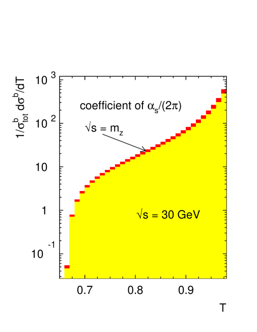
Figure 13: Coefficient $c_{1}$ of the thrust distribution (6.7) for $b$ quarks at $\sqrt{s}=m_{Z}$ (upper curve) and $\sqrt{s}=30$ GeV (lower curve).

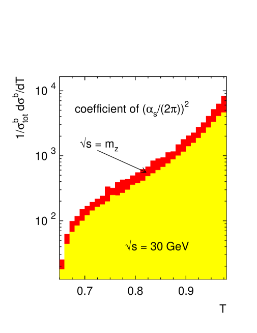
Figure 14: Coefficient $c_{2}$ of the thrust distribution (6.7) for $b$ quarks at $\sqrt{s}=m_{Z}$ (upper curve) and $\sqrt{s}=30$ GeV (lower curve).

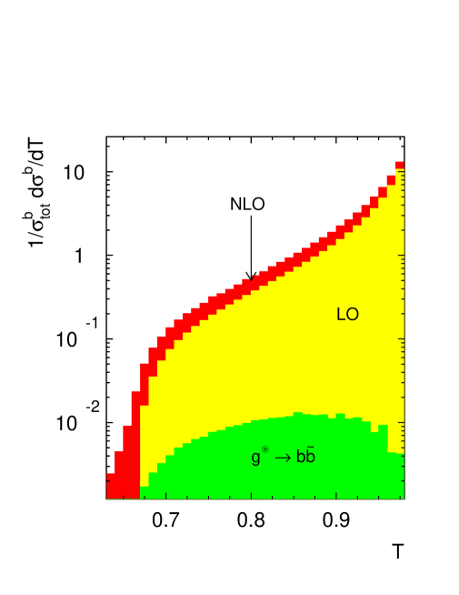
Figure 15: The thrust distribution (6.7) at $\sqrt{s}=30$ GeV. Shown separately is the contribution from the process $e^{+}e^{-}\to q\bar{q}g^{\ast}\to q\bar{q}b\bar{b}$.

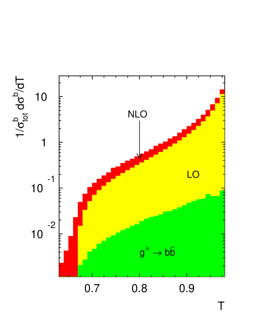
Figure 16: Same as Fig. 15, but at $\sqrt{s}=m_{Z}$.

In the massless calculation at $\mu=\sqrt{s}$, the coefficients $c_{1}$ and $c_{2}$ are independent of the c.m. energy. This changes in the massive case as shown in Figs. 13 and 14. For these and the following plots of the thrust distribution we exclude the singular two-jet region near $T=1$. We use a slicing parameter $s_{min}=1{\mbox{\ GeV}}^{2}$. We now only require the tagging of one $b$ quark and omit the contributions from the process $e^{+}e^{-}\to q\bar{q}g^{\ast}\to q\bar{q}b\bar{b}$. In Fig. 15 we plot the thrust distribution (6.7) at $\sqrt{s}=\mu=30$ GeV with $\alpha_{s}(\mu=\sqrt{s})=0.142$ and $m^{\scriptsize{\mbox{${\overline{\mbox{MS}}}$}}}_{b}(\mu=\sqrt{s})=3.33$ GeV. Shown separately (and not included in the NLO histogram) is the contribution from $e^{+}e^{-}\to q\bar{q}g^{\ast}\to q\bar{q}b\bar{b}$ calculated “naively”, i.e. directly from the matrix element without imposing cuts. The LO and NLO thrust distributions for $b$ quarks at $\sqrt{s}=m_{Z}$ depicted in Fig. 16 are almost identical to the corresponding distributions at $\sqrt{s}=30$ GeV. The reason is that the change in the coefficients $c_{1,2}$ due to mass effects as exhibited in Figs. 13 and 14 is almost exactly compensated by the larger value of $\alpha_{s}$ at $\mu=30$ GeV. The contribution from $g^{\ast}\to b\bar{b}$ splitting is bigger at the higher energy scale.

7 Summary

In view of the large number of jet events collected both at LEP and SLC it is desirable for precision tests of QCD to use NLO partonic matrix elements that include the full quark mass dependence. We have presented in this article the necessary ingredients to calculate any jet quantity that gets contributions from three- and four jet final states involving massive quarks at order $\alpha_{s}^{2}$. In particular, we have derived an explicit analytic expression for the virtual corrections to $e^{+}e^{-}\to Q\bar{Q}g$. Our approach involves a modification of the phase space slicing method incorporating massive quarks. The independence of physical quantities on the slicing parameter $s_{min}$ is a crucial test of the overall consistency and has been carefully checked. As to numerical results we have evaluated the three jet fraction for $b$ quarks and compared it to the inclusive three jet fraction evaluated for massless quarks at different c.m. energies. We have further studied the dependence of our results on the renormalization scale. If we take this dependence as an estimate of the neglected higher order corrections, we may conclude that they are of moderate size, in particular in the case of jet rates computed using the Durham algorithm. A particularly interesting quantity to study mass effects is the differential two jet rate. At the $Z$ pole and for small $y_{cut}$, the effects of the $b$ quark mass are of the order of 5% or larger. As a final example we studied the thrust distribution for $b$ quark samples at $\sqrt{s}=m_{Z}$ and $\sqrt{s}=30$ GeV. Future work will include the calculation of several other three jet quantities, in particular also parity violating observables.

Appendix A Appendix

In (4.8), we defined the finite contributions $F_{1}^{{\rm lc},VV(AA)}$ and $F_{1}^{{\rm sc},VV(AA)}$ to the function $F_{1}^{{\rm virtual},VV(AA)}$, which are generated by the interference of the loop diagrams Figs. 2(a)-(k) with the Born graphs. In this appendix, we give explicit expressions for these contributions in terms of finite parts of one-loop integrals times coefficient functions. For the two- and three-point loop integrals we use the notation of [40], i.e. all integrals are labelled with respect to the following box integrals:

$$D_{0} = \frac{1}{i\pi^{2}}\int\!\!\frac{\left(2\pi\mu\right)^{-2\epsilon}d^{4-2\epsilon}l}{(l^{2}+i\varepsilon)((l+k_{3})^{2}+i\varepsilon)((l+k_{13})^{2}-m^{2}+i\varepsilon)((l-k_{2})^{2}-m^{2}+i\varepsilon)},$$

$$D_{0}^{{\rm sc},1} = \frac{1}{i\pi^{2}}\int\!\!\frac{\left(2\pi\mu\right)^{-2\epsilon}d^{4-2\epsilon}l}{(l^{2}+i\varepsilon)((l+k_{1})^{2}-m^{2}+i\varepsilon)((l+k_{13})^{2}-m^{2}+i\varepsilon)((l-k_{2})^{2}-m^{2}+i\varepsilon)},$$

$$D_{0}^{{\rm sc},2} = D_{0}^{{\rm sc},1}\big{|}_{k_{1}\leftrightarrow k_{2}},$$ (A.1)

with $k_{1}^{2}=k_{2}^{2}=m^{2}$, $k_{3}^{2}=0$, and $k_{13}=k_{1}+k_{3}$. In the following, $C_{0}(1,2,3)$ denotes the integral obtained from $D_{0}$ by omitting the fourth denominator, etc. The nonvanishing one-point function is defined by $A(zs)=(2\pi\mu)^{-2\epsilon}\int\!\!d^{d}l[l^{2}-m^{2}+i\varepsilon]^{-1}$. As stated in section 4, we eliminate the above scalar box integrals in $d=4-2\epsilon$ dimensions in favor of the box integrals in $d=6-2\epsilon$ dimensions.

We write

$$F_{1}^{{\rm lc},VV(AA)} = d_{d=6}^{VV(AA)}{\mbox{Re}}\,D_{0}^{d=6}$$ (A.2)

$$+ c_{123}^{VV(AA)}{\mbox{Re}}\,\overline{C}_{0}(1,2,3)+c_{124}^{VV(AA)}{\mbox{Re}}\,\overline{C}_{0}(1,2,4)$$

$$+ c_{134}^{{\rm lc},VV(AA)}{\mbox{Re}}\,C_{0}(1,3,4)+c_{234}^{{\rm lc},VV(AA)}{\mbox{Re}}\,C_{0}(2,3,4)$$

$$+ b_{13}^{{\rm lc},VV(AA)}{\mbox{Re}}\,\overline{B}_{0}(1,3)+b_{24}^{{\rm lc},VV(AA)}{\mbox{Re}}\,\overline{B}_{0}(2,4)$$

$$+ b_{14}^{{\rm lc},VV(AA)}{\mbox{Re}}\,\overline{B}_{0}(1,4)+b_{34}^{{\rm lc},VV(AA)}{\mbox{Re}}\,\overline{B}_{0}(3,4)$$

$$+ a^{{\rm lc},VV(AA)}{\mbox{Re}}\,\overline{A}+k^{{\rm lc},VV(AA)}.$$

$$F_{1}^{{\rm sc},VV(AA)} = \tilde{d}_{d=6}^{VV(AA)}{\mbox{Re}}\,D_{0}^{{\rm sc},1,d=6}+\tilde{d^{\prime}}_{d=6}^{VV(AA)}{\mbox{Re}}\,D_{0}^{{\rm sc},2,d=6}$$ (A.3)

$$+ \tilde{c}_{123}^{VV(AA)}{\mbox{Re}}\,C_{0}^{{\rm sc},1}(1,2,3)+\tilde{c}_{134}^{VV(AA)}{\mbox{Re}}\,C_{0}^{{\rm sc},2}(1,3,4)$$

$$+ \tilde{c}_{124}^{VV(AA)}{\mbox{Re}}\,\overline{C}_{0}^{{\rm sc},1}(1,2,4)+c_{134}^{{\rm sc},VV(AA)}{\mbox{Re}}\,C_{0}(1,3,4)$$

$$+ c_{234}^{{\rm sc},VV(AA)}{\mbox{Re}}\,C_{0}(2,3,4)+\tilde{c}_{234}^{VV(AA)}{\mbox{Re}}\,C_{0}^{{\rm sc},1}(2,3,4)$$

$$+ b_{13}^{{\rm sc},VV(AA)}{\mbox{Re}}\,\overline{B}_{0}(1,3)+b_{24}^{{\rm sc},VV(AA)}{\mbox{Re}}\,\overline{B}_{0}(2,4)$$

$$+ b_{14}^{{\rm sc},VV(AA)}{\mbox{Re}}\,\overline{B}_{0}(1,4)+b_{34}^{{\rm sc},VV(AA)}{\mbox{Re}}\,\overline{B}_{0}(3,4)$$

$$+ \tilde{b}_{24}^{VV(AA)}{\mbox{Re}}\,\overline{B}^{{\rm sc},1}_{0}(2,4)+a^{{\rm sc},VV(AA)}{\mbox{Re}}\,\overline{A}+k^{{\rm sc},VV(AA)}.$$

The symbol $\overline{I}$ means that the finite part of the UV or IR divergent integral $I$ is to be taken.

The real parts of the integrals appearing in (A.2) and (A.3) read (recall that $z=m^{2}/s,\ x_{g}=2-x-\bar{x}$):

$${\mbox{Re}}\,D_{0}^{d=6} = \frac{\pi}{sx_{g}}\Bigg{\{}\frac{(1-\bar{x})\alpha}{(\alpha-x_{+}^{s})(\alpha-x_{-}^{s})}\left[-\frac{\pi^{2}}{6}+\mbox{Li}_{2}\left(\frac{\alpha-1}{\alpha}\right)\right]$$ (A.4)

$$+ \frac{(1-\bar{x})x_{+}^{s}}{(\alpha-x_{+}^{s})(x_{+}^{s}-x_{-}^{s})}\Bigg{[}\,\frac{\pi^{2}}{6}-\mbox{Li}_{2}\left(\frac{x_{+}^{s}-1}{x_{+}^{s}}\right)+\mbox{Li}_{2}\left(\frac{x_{+}^{s}-1}{x_{+}^{s}-\rho}\right)$$

$$+ \mbox{Li}_{2}\left(\frac{x_{+}^{s}-\rho}{x_{+}^{s}}\right)-\mbox{Li}_{2}\left(\frac{1-\rho-x_{+}^{s}}{1-x_{+}^{s}}\right)-\mbox{Li}_{2}\left(\frac{-x_{+}^{s}}{1-x_{+}^{s}-\rho}\right)$$

$$+ \frac{1}{2}\ln^{2}\left(\frac{x_{+}^{s}}{x_{+}^{s}-\rho}\right)-\frac{1}{2}\ln^{2}\left(\frac{1-x_{+}^{s}}{1-\rho-x_{+}^{s}}\right)\,\Bigg{]}$$

$$+ \frac{(1-\bar{x})x_{-}^{s}}{(\alpha-x_{-}^{s})(x_{-}^{s}-x_{+}^{s})}\Bigg{[}\,\frac{\pi^{2}}{6}-\mbox{Li}_{2}\left(\frac{x_{-}^{s}-1}{x_{-}^{s}}\right)+\mbox{Li}_{2}\left(\frac{x_{-}^{s}-1}{x_{-}^{s}-\rho}\right)$$

$$+ \mbox{Li}_{2}\left(\frac{x_{-}^{s}-\rho}{x_{-}^{s}}\right)-\mbox{Li}_{2}\left(\frac{1-\rho-x_{-}^{s}}{1-x_{-}^{s}}\right)-\mbox{Li}_{2}\left(\frac{-x_{-}^{s}}{1-x_{-}^{s}-\rho}\right)$$

$$+ \frac{1}{2}\ln^{2}\left(\frac{x_{-}^{s}}{x_{-}^{s}-\rho}\right)-\frac{1}{2}\ln^{2}\left(\frac{1-x_{-}^{s}}{1-\rho-x_{-}^{s}}\right)\,\Bigg{]}\Bigg{\}}$$

$$+ (x\leftrightarrow\bar{x}),$$

$$\mbox{Re}\,C_{0}(1,2,3) = \frac{1}{2s}\frac{1}{1-\bar{x}}\Bigg{\{}\frac{1}{\epsilon^{2}}-\frac{1}{\epsilon}\left[\gamma+\ln\left(\frac{sz(\zeta-1)^{2}}{4\pi\mu^{2}}\right)\right]$$ (A.5)

$$- \frac{1}{12}\Bigg{(}15\pi^{2}+24\,\mbox{Li}_{2}\left(\frac{1}{\zeta}\right)+12\ln^{2}(\zeta)$$

$$- 6\left[\gamma+\ln\left(\frac{sz(\zeta-1)^{2}}{4\pi\mu^{2}}\right)\right]^{2}\Bigg{)}\Bigg{\}},$$

$$\mbox{Re}\,C_{0}(1,2,4) = \mbox{Re}\,C_{0}(1,2,3)\Big{|}_{x\leftrightarrow\bar{x}},$$ (A.6)

$$\mbox{Re}\,C_{0}(1,3,4) = -\frac{1}{s}\frac{1}{x_{+}^{s}-x_{-}^{s}}\,\Bigg{\{}-\frac{1}{2}\ln^{2}\left(\frac{x_{+}^{s}}{x_{+}^{s}-\rho}\right)+\frac{1}{2}\ln^{2}\left(\frac{x_{+}^{s}-1}{x_{+}^{s}+\rho-1}\right)$$ (A.7)

$$- \mbox{Li}_{2}\left(\frac{x_{+}^{s}-1}{x_{+}^{s}-\rho}\right)+\mbox{Li}_{2}\left(\frac{x_{+}^{s}}{x_{+}^{s}+\rho-1}\right)+\mbox{Li}_{2}\left(\frac{x_{+}^{s}-1}{x_{+}^{s}}\right)$$

$$- \mbox{Li}_{2}\left(\frac{x_{+}^{s}-\rho}{x_{+}^{s}}\right)+\mbox{Li}_{2}\left(\frac{x_{+}^{s}+\rho-1}{x_{+}^{s}-1}\right)\Bigg{\}}+(x_{+}^{s}\leftrightarrow x_{-}^{s}),$$

$$\mbox{Re}\,C_{0}(2,3,4) = \mbox{Re}\,C_{0}(1,3,4)\Big{|}_{x\leftrightarrow\bar{x}},$$ (A.8)

$$\mbox{Re}\,B_{0}(1,3) = \frac{1}{\epsilon}-\gamma-\ln\left(\frac{z\zeta s}{4\pi\mu^{2}}\right)+\frac{\zeta-1}{\zeta}\ln\left(\frac{\zeta}{\zeta-1}\right)+\frac{1}{\zeta}\ln(\zeta)+2,$$ (A.9)

$$\mbox{Re}\,B_{0}(2,4) = \mbox{Re}\,B_{0}(1,3)\Big{|}_{x\leftrightarrow\bar{x}},$$ (A.10)

$$\mbox{Re}\,B_{0}(1,4) = \frac{1}{\epsilon}-\gamma-\ln\left(\frac{zs}{4\pi\mu^{2}}\right)+2,$$ (A.11)

$$\mbox{Re}\,B_{0}(3,4) = \frac{1}{\epsilon}-\gamma-\ln\left(\frac{zs}{4\pi\mu^{2}}\right)+2+(1-2\rho)\ln\left(\frac{\rho}{1-\rho}\right),$$ (A.12)

$$\mbox{Re}\,A(zs) = zs\left(\frac{1}{\epsilon}-\gamma-\ln\left(\frac{zs}{4\pi\mu^{2}}\right)+1\right),$$ (A.13)

$$\mbox{Re}\,C_{0}^{{\rm sc},1}(1,2,4) = \frac{1}{s}\,\frac{1}{1-x_{g}}\,\,\frac{1}{1-2\eta}\Bigg{\{}\,\frac{1}{\epsilon}\,\ln\left(\frac{\eta}{1-\eta}\right)$$ (A.14)

$$- 2\,\mbox{Li}_{2}\left(\frac{\eta}{1-\eta}\right)-\frac{1}{2}\ln^{2}\left(\frac{\eta}{1-\eta}\right)-\frac{2}{3}\pi^{2}$$

$$- \ln\left(\frac{\eta}{1-\eta}\right)\left[\gamma+\ln\left(\frac{(1-x_{g})s}{4\pi\mu^{2}}\right)+2\ln(1-2\eta)\right]\Bigg{\}},$$

$$\mbox{Re}\,C_{0}^{{\rm sc},1}(1,2,3) = \frac{1}{s}\,\frac{1}{1-\bar{x}}\left\{\mbox{Li}_{2}\left(\frac{1}{\zeta}\right)+\frac{1}{2}\ln^{2}(\zeta)-\frac{\pi^{2}}{6}\right\},$$

$$\mbox{Re}\,C_{0}^{{\rm sc},2}(1,3,4) = \mbox{Re}\,C_{0}^{{\rm sc},1}(1,2,3)\Big{|}_{x\leftrightarrow\bar{x}},$$ (A.15)

$$\mbox{Re}\,C_{0}^{{\rm sc},1}(2,3,4) = \frac{1}{sx_{g}}\Bigg{\{}\frac{1}{2}\ln^{2}\left(\frac{\rho}{1-\rho}\right)-\frac{1}{2}\ln^{2}\left(\frac{\eta}{1-\eta}\right)\Bigg{\}},$$ (A.16)

$${\mbox{Re}}\,D_{0}^{{\rm sc},1,d=6} = \frac{\pi}{2[(1-x_{g})(1-x)(1-\bar{x})-zx_{g}^{2}]}$$ (A.17)

$$\times \bigg{\{}(1-\bar{x})(1-x_{g})(1-x_{g}-4z)$$

$$\times [-s(1-\bar{x})\mbox{Re}\,D_{0}^{{\rm sc},1,d=4-2\epsilon}+\mbox{Re}\,C_{0}^{{\rm sc},1}(1,2,4)]$$

$$+ [(1-\bar{x})(1-x_{g})-2zx_{g}]$$

$$\times [(1-\bar{x})\mbox{Re}\,C_{0}^{{\rm sc},1}(1,2,3)-x_{g}\mbox{Re}\,C_{0}^{{\rm sc},1}(2,3,4)]$$

$$+ (1-\bar{x})[-\bar{x}(1-x_{g})+2z(x+\bar{x})]\mbox{Re}\,C_{0}(1,3,4)\bigg{\}},$$

$${\mbox{Re}}\,D_{0}^{{\rm sc},2,d=6} = {\mbox{Re}}\,D_{0}^{{\rm sc},1,d=6}\Big{|}_{x\leftrightarrow\bar{x}},$$ (A.18)

$$\mbox{Re}\,B_{0}^{{\rm sc},1}(2,4) = \frac{1}{\epsilon}-\gamma-\ln\left(\frac{zs}{4\pi\mu^{2}}\right)+2+(1-2\eta)\ln\left(\frac{\eta}{1-\eta}\right),$$ (A.19)

where

$$\alpha = \frac{1-x}{x_{g}},$$ (A.20)

$$\zeta = \frac{1-\bar{x}+z}{z},$$ (A.21)

$$\rho = \frac{1}{2}(1-\sqrt{1-4z}),$$ (A.22)

$$x_{\pm}^{s} = \frac{1}{2}(\bar{x}\pm\sqrt{\bar{x}^{2}-4z}),$$ (A.23)

$$x_{\mp}^{t} = 1-\frac{1}{2}(x\pm\sqrt{x^{2}-4z}),$$ (A.24)

$$\eta = \frac{1}{2}\left(1-\sqrt{1-\frac{4z}{1-x_{g}}}\right),$$ (A.25)

and (cf. [57])

$$\mbox{Re}\,D_{0}^{{\rm sc},1,d=4-2\epsilon} = \frac{1}{s^{2}}\,\frac{1}{1-\bar{x}}\,\frac{1}{1-x_{g}}\,\frac{1}{1-2\eta}$$ (A.26)

$$\times \Bigg{\{}\left[\frac{1}{\epsilon}-\gamma-\ln\left(\frac{sz(\zeta-1)^{2}}{4\pi\mu^{2}}\right)\right]\ln\left(\frac{\eta}{1-\eta}\right)-\pi^{2}$$

$$- 2\,\mbox{Li}_{2}\left(1-\frac{\eta}{1-\eta}\frac{\rho}{1-\rho}\right)-2\,\mbox{Li}_{2}\left(1-\frac{\eta}{1-\eta}\frac{1-\rho}{\rho}\right)$$

$$+ \mbox{Li}_{2}\left(1-\frac{\eta^{2}}{(1-\eta)^{2}}\right)-\ln^{2}\left(\frac{\rho}{1-\rho}\right)\Bigg{\}}.$$

The coefficient functions read (where $B=1/(1-x)/(1-\bar{x})$, and $\beta$ and $\omega$ have been defined in (4.9)):

$$d_{d=6}^{VV}\ = \ \frac{sB[1-x_{g}-zx_{g}^{2}B]}{\pi}\bigg{\{}x^{2}$$

$$+ \ 4zB\left[-2x^{2}+5x+x\bar{x}(x-2)-2-z(2x^{2}+3(1-2x)+x\bar{x})\right]+({x\leftrightarrow\bar{x}})\bigg{\}},$$

$$c_{123}^{VV}\ = \ -\frac{s}{1-x}\bigg{\{}x^{2}+2zB[-3x^{2}+8x+2x\bar{x}(x-2)-3-zx_{g}^{2}]+({x\leftrightarrow\bar{x}})\bigg{\}},$$

$$c_{124}^{VV}\ = \ c_{123}^{VV}\Big{|}_{x\leftrightarrow\bar{x}},$$

$$c_{134}^{{\rm lc},VV}\ = \ -\frac{zs}{1-x}\bigg{\{}\frac{-4z(1+2z)}{1-\bar{x}}-\frac{2x^{2}+2x\bar{x}-12x+9-4\bar{x}-\bar{x}^{2}}{1-x}$$

$$- \ \frac{z[13x^{2}-34x-12\bar{x}+8x\bar{x}+25-8z(2x+\bar{x}-3)]}{(1-x)^{2}}$$

$$+ \frac{1}{\bar{x}^{2}-4z}[-x^{2}-x^{2}\bar{x}+8x-6x\bar{x}+9\bar{x}-7$$

$$+ z(36x-x^{2}-60+29\bar{x}-10x\bar{x})+8z^{2}(x+\bar{x}-6)]$$

$$- \ \frac{3}{(\bar{x}^{2}-4z)^{2}}[-(1-x)^{2}\bar{x}+z(8x^{2}-20x-16\bar{x}+20x\bar{x}-5x^{2}\bar{x}+12)$$

$$+ \ 4z^{2}(x^{2}-10x-5\bar{x}+2x\bar{x}+12)+16z^{3}]\bigg{\}},$$

$$c_{234}^{{\rm lc},VV}\ = \ c_{134}^{{\rm lc},VV}\Big{|}_{x\leftrightarrow\bar{x}},$$

$$b_{13}^{{\rm lc},VV}\ = \ \frac{3z}{1-x}-\frac{z(1-x)}{2(1-\bar{x})^{2}}+\frac{-1+2z(5-2x)+4z^{2}(x-4)+16z^{3}}{2(1-\bar{x})(1-4z)}$$

$$- \ \frac{-1+x+2z(1-x)+z^{2}(x-2)+2z^{3}}{2(1-\bar{x}+z)(1-z)(1-x)}+\frac{1}{2(1-x)(1-z)(1-4z)(\bar{x}^{2}-4z)}$$

$$\times \ [-(1-x)(1-x_{g}+3x\bar{x})+z(37-26x+14x\bar{x}-11x^{2}\bar{x}-2x^{2}-18\bar{x})$$

$$+ \ z^{2}(124x+4x^{2}\bar{x}-112+x^{2}+100\bar{x}-48x\bar{x})$$

$$+ \ 2z^{3}(-120+2x^{2}\bar{x}+5\bar{x}+10x\bar{x})+8z^{4}(2x\bar{x}+32-12x-11\bar{x})+64z^{5}]$$

$$- \frac{3z}{(1-x)(\bar{x}^{2}-4z)^{2}}[(1-x)(2x-3x\bar{x}+5\bar{x}-2)$$

$$+ \ z(-6x^{2}-12x\bar{x}+x^{2}\bar{x}+28x+16\bar{x}-24)+4z^{2}(-6+2x+\bar{x})],$$

$$b_{24}^{{\rm lc},VV}\ = \ b_{13}^{{\rm lc},VV}\Big{|}_{x\leftrightarrow\bar{x}},$$

$$b_{14}^{{\rm lc},VV}\ = \ -\frac{B}{16}\bigg{\{}2x^{5}-3x^{4}-x^{3}-40x+x\bar{x}(2x^{3}+2x^{2}+5x\bar{x}-43x+36)+8$$

$$+ \ 8zB[-x^{4}+7x^{3}+8x^{2}-48x+x\bar{x}(x^{3}+x^{2}\bar{x}-4x^{2}-3x\bar{x}-x+20)+20]$$

$$+ \ 64z^{2}B^{2}[-3x^{3}+12x^{2}-18x+x\bar{x}(x^{2}\bar{x}+x^{2}-8x-x\bar{x}+11)+5]$$

$$+ \ 128z^{3}B^{2}x_{g}(1-x)^{2}\bigg{\}}$$

$$+ \ \frac{xB}{8(x^{2}-4z)}[x^{6}-8x^{4}+24x^{3}-30x^{2}+22x-6$$

$$+ \ \bar{x}(x^{5}+4x^{4}-27x^{3}+48x^{2}-44x+12)+\bar{x}^{2}(4x^{3}-17x^{2}+22x-6)]$$

$$+ \ \frac{3x^{3}[x^{2}+x\bar{x}-2(1-x_{g})]^{2}}{16(1-\bar{x})(x^{2}-4z)^{2}}+(x\leftrightarrow\bar{x}),$$

$$b_{34}^{{\rm lc},VV}\ = \ \frac{B}{8}\bigg{\{}2x^{4}+x\bar{x}(2x^{2}+x-6)-5x^{3}-2x^{2}-12x+8$$

$$+ \ 8zB[x\bar{x}(x^{2}+x\bar{x}-11x+16)-x^{3}+12x^{2}-28x+10+2zx_{g}^{2}]$$

$$- \ \frac{1}{x^{2}-4z}[2x^{6}-2x^{5}-7x^{4}+28x^{3}-36x^{2}+28x-8$$

$$+ \ 2\bar{x}(x^{5}+2x^{4}-18x^{3}+32x^{2}-30x+8)+\bar{x}^{2}(6x^{3}-25x^{2}+32x-8)]\bigg{\}}$$

$$- \ \frac{3x^{2}[x^{2}+x\bar{x}-2(1-x_{g})]^{2}}{8(1-\bar{x})(x^{2}-4z)^{2}}+(x\leftrightarrow\bar{x}),$$

$$a^{{\rm lc},VV}\ = \ \frac{B}{2s}\bigg{\{}B[-11x^{2}+24x+2x\bar{x}(4x-7)-7]+4zB^{2}[4x^{3}-2x^{2}\bar{x}^{2}-16x^{2}+23x$$

$$+ x\bar{x}(-3x^{2}+17x-17)-6-2zx_{g}(1-x)^{2}]-\frac{[x^{2}+x\bar{x}-2(1-x_{g})]^{2}}{(2-x)(x^{2}-4z)}$$

$$- \frac{2x^{3}-8x^{2}+12x-7+\bar{x}(2-x)^{2}}{(2-x)(1-x+z)}+(x\leftrightarrow\bar{x})\bigg{\}},$$

$$k^{{\rm lc},VV}\ = \ -\frac{1}{2}x_{g}^{2}B\left[\gamma-\ln\left(\frac{4\pi z\mu^{2}}{s(1-x)^{2}}\right)\right]+\frac{B}{8}\bigg{\{}x^{3}-16x^{2}+24x+3x\bar{x}(x-4)-8$$ (A.27)

$$+ 4zB[5x^{3}-15x^{2}+20x+x\bar{x}(7x-12)-5]$$

$$+ 16z^{2}B^{2}[-4x^{3}+2x^{2}\bar{x}^{2}+16x^{2}-23x+x\bar{x}(3x^{2}-17x+17)+6$$

$$+ 2zx_{g}(1-x)^{2}]-\frac{x[x^{2}+x\bar{x}-2(1-x_{g})]^{2}}{x^{2}-4z}\bigg{\}}+(x\leftrightarrow\bar{x}).$$

$$d_{d=6}^{AA}\ = \ d_{d=6}^{VV}+\frac{2zBs[1-x_{g}-zBx_{g}^{2}]}{\pi}\bigg{\{}x^{2}-10x+x\bar{x}+5$$

$$+ \ 6zB(2x^{2}-6x+x\bar{x}+3)+(x\leftrightarrow\bar{x})\bigg{\}},$$

$$c_{123}^{AA}\ = \ c_{123}^{VV}-\frac{2zs}{1-x}\bigg{\{}x^{2}-10x+x\bar{x}+5+3zBx_{g}^{2}+(x\leftrightarrow\bar{x})\bigg{\}},$$

$$c_{124}^{AA}\ = \ c_{123}^{AA}\Big{|}_{x\leftrightarrow\bar{x}},$$

$$c_{134}^{{\rm lc},AA}\ = \ c_{134}^{{\rm lc},VV}+\frac{6zs}{1-x}\bigg{\{}-\frac{4z^{2}}{1-\bar{x}}-\frac{z(x^{2}+\bar{x}^{2}-16(x+\bar{x})+2x\bar{x}+16)}{3(1-x)}$$

$$- \ \frac{-(1-x)^{2}(1-\bar{x})+2z(1-x)(3x+\bar{x}-9)+2z^{2}(2x-\bar{x}-7)}{3(\bar{x}^{2}-4z)}$$

$$+ \ \frac{12z^{2}(2x+\bar{x}-3)}{3(1-x)^{2}}-\frac{2z}{(\bar{x}^{2}-4z)^{2}}[(1-x)(x+3\bar{x}-2x\bar{x}-1)$$

$$+ \ z(-5x^{2}+x^{2}\bar{x}+20x+12\bar{x}-10x\bar{x}-16)+4z^{2}(2x+\bar{x}-5)]\bigg{\}},$$

$$c_{234}^{{\rm lc},AA}\ = \ c_{134}^{{\rm lc},AA}\Big{|}_{x\leftrightarrow\bar{x}},$$

$$b_{13}^{{\rm lc},AA}\ = \ b_{13}^{{\rm lc},VV}-z\bigg{\{}\frac{1+z}{1-x}+\frac{1-2z+8z^{2}}{(1-\bar{x})(1-4z)}+\frac{z(1-x)}{(1-\bar{x})^{2}}+\frac{(1-z)(1-x)-z^{2}}{(1-x)(1-\bar{x}+z)(1-z)}$$

$$+ \ \frac{1}{(1-x)(\bar{x}^{2}-4z)(1-z)(1-4z)}[-6x^{2}+14x-2x\bar{x}+\bar{x}-8$$

$$+ \ 2z(15x^{2}-31x+5x\bar{x}-4\bar{x}+13)+2z^{2}(-12x^{2}-12x\bar{x}+17\bar{x}+28)$$

$$+ \ 4z^{3}(4x\bar{x}+12x-6\bar{x}-21)+16z^{4}]$$

$$+ \ \frac{6}{(1-x)(\bar{x}^{2}-4z)^{2}}[(1-x)^{2}\bar{x}+z(-6x^{2}+3x^{2}\bar{x}+16x-14x\bar{x}+12\bar{x}-10)$$

$$+ \ 2z^{2}(-x^{2}+12x-2x\bar{x}+6\bar{x}-16)-8z^{3}]\bigg{\}},$$

$$b_{24}^{{\rm lc},AA}\ = \ b_{13}^{{\rm lc},AA}\Big{|}_{x\leftrightarrow\bar{x}},$$

$$b_{14}^{{\rm lc},AA}\ = \ b_{14}^{{\rm lc},VV}+\frac{z}{4}\bigg{\{}-\frac{3x^{2}[x^{2}+x\bar{x}-2(1-x_{g})]^{2}}{(1-\bar{x})(x^{2}-4z)^{2}}+B(7x^{3}-14x^{2}+13x^{2}\bar{x}$$

$$- 14x\bar{x}-52x+24)-16zB^{2}(x^{3}-13x^{2}+x^{2}\bar{x}-8x\bar{x}+33x-14)$$

$$+ 96z^{2}B^{3}x_{g}(1-x)^{2}-\frac{2B}{x^{2}-4z}[5x^{5}-19x^{4}+34x^{3}-30x^{2}+14x-2$$

$$+ \ 2\bar{x}(2x^{2}-3x+2)(2x^{2}-4x+1)-\bar{x}^{2}(1-x)(3x^{2}-6x+2)]+(x\leftrightarrow\bar{x})\bigg{\}},$$

$$b_{34}^{{\rm lc},AA}\ = \ b_{34}^{{\rm lc},VV}+\frac{z}{2}\bigg{\{}\frac{3x[x^{2}+x\bar{x}-2(1-x_{g})]^{2}}{(1-\bar{x})(x^{2}-4z)^{2}}-2B(3x^{2}-20x+3x\bar{x}+10)$$

$$- \ 8zB^{2}x_{g}^{2}+\frac{B}{x^{2}-4z}[8x^{4}-29x^{3}+48x^{2}-36x+12$$

$$+ \ 2\bar{x}(6x^{3}-19x^{2}+20x-8)+\bar{x}^{2}(4x^{2}-9x+4)]+(x\leftrightarrow\bar{x})\bigg{\}},$$

$$a^{{\rm lc},AA}\ = \ a^{{\rm lc},VV}+\frac{1}{s}\bigg{\{}-\frac{x^{2}-x-x\bar{x}+2\bar{x}-1}{(1-x+z)(2-x)(1-\bar{x})}$$

$$+ \frac{B}{2}[x^{2}-10x+x\bar{x}+3+4zB(7x^{2}-19x+4x\bar{x}+8)+24z^{2}x_{g}B^{2}(1-x)^{2}]$$

$$+ \ \frac{xB[x^{2}+x\bar{x}-2(1-x_{g})]^{2}}{2(2-x)(x^{2}-4z)}+(x\leftrightarrow\bar{x})\bigg{\}},$$

$$k^{{\rm lc},AA}\ = \ k^{{\rm lc},VV}+\frac{zB}{2}\bigg{\{}-2x_{g}^{2}\left[\gamma-\ln\left(\frac{4\pi z\mu^{2}}{s(1-x)^{2}}\right)\right]+\frac{[x^{2}+x\bar{x}-2(1-x_{g})]^{2}}{x^{2}-4z}$$

$$- \ 10x^{2}+40x-10x\bar{x}-7+2zB(5x^{3}-52x^{2}+15x^{2}\bar{x}+130x-46x\bar{x}-52)$$

$$- \ 24z^{2}B^{2}x_{g}(1-x)^{2}+(x\leftrightarrow\bar{x})\bigg{\}}.$$ (A.28)

$$\tilde{d}_{d=6}^{VV}\ = \ -\frac{s[1-x_{g}-zBx_{g}^{2}]}{\pi(1-\bar{x})(1-x_{g}-4z)}\bigg{\{}x^{2}+2\bar{x}^{2}-2x-2\bar{x}+2x\bar{x}+1$$

$$- \ \frac{2z}{(1-\bar{x})(1-x_{g})}[-3x^{2}-4\bar{x}^{2}+7x+9\bar{x}-5+x\bar{x}(x+\bar{x}-6)$$

$$+ \ 4z(-x^{2}-3\bar{x}^{2}+5x+8\bar{x}-3x\bar{x}-6)-8z^{2}x_{g}]\bigg{\}},$$

$$\tilde{d^{\prime}}_{d=6}^{VV}\ = \ \tilde{d}_{d=6}^{VV}\Big{|}_{x\leftrightarrow\bar{x}},$$

$$\tilde{c}_{123}^{VV}\ = \ -\frac{zs}{2}\bigg{\{}\frac{2(2-\bar{x}+z)}{1-x}+\frac{2z(1-x)[x(x-4)+4z(-3x+2)+16z^{2}]}{(1-\bar{x})^{2}(x-4z)x}$$

$$- \ \frac{(2x-1-4z)[(x-8z)(2x^{2}-2x+1)+8z^{2}(8x-3)-96z^{3}]}{(1-x)(1-x_{g}-4z)(x-4z)^{2}}$$

$$+ \ \frac{2}{(1-\bar{x})(x-4z)^{2}x^{2}}[x^{3}(x^{2}+x+1)+2zx^{2}(2x^{2}-4x-5)-8z^{2}x(8x^{2}-3x-3)$$

$$+ \ 32z^{3}(5x^{2}-1)-64z^{4}(x+1)]-\frac{x(2x-1)+4z(1+x^{2})+8z^{2}}{(1-x)(1-x_{g})x^{2}}\bigg{\}},$$

$$\tilde{c}_{134}^{VV}\ = \ \tilde{c}_{123}^{VV}\Big{|}_{x\leftrightarrow\bar{x}},$$

$$\tilde{c}_{124}^{VV}\ = \ sB(1-x_{g}-2z)$$

$$\times \ \bigg{\{}x^{2}+2zB[-3x^{2}+2x^{2}\bar{x}-4x\bar{x}+8x-3-zx_{g}^{2}]+(x\leftrightarrow\bar{x})\bigg{\}},$$

$$c_{134}^{{\rm sc},VV}\ = \ \tilde{c}_{123}^{VV}-zs\bigg{\{}-\frac{z(1-x)(x-8z-4)}{(1-\bar{x})^{2}x}+\frac{x(2x-1)+4z(x^{2}+1)+8z^{2}}{(1-x)(1-x_{g})x^{2}}$$

$$+ \ \frac{1}{(1-x)(\bar{x}^{2}-4z)}[x^{2}+x^{2}\bar{x}-6x-5\bar{x}+3x\bar{x}+5$$

$$+ \ z(x^{2}-32x-25\bar{x}+10x\bar{x}+48)-8z^{2}(x+\bar{x}-6)]$$

$$+ \ \frac{3z}{(1-x)(\bar{x}^{2}-4z)^{2}}[8x^{2}-5x^{2}\bar{x}-20x-16\bar{x}+20x\bar{x}+12$$

$$+ \ 4z(x^{2}-10x-5\bar{x}+2x\bar{x}+12)+16z^{2}]$$

$$- \ \frac{3\bar{x}(1-x)}{(\bar{x}^{2}-4z)^{2}}-\frac{x(x^{2}+x+1)+2z(5x^{2}-2x-2)-8z^{2}(x+1)}{(1-\bar{x})x^{2}}\bigg{\}},$$

$$c_{234}^{{\rm sc},VV}\ = \ c_{134}^{{\rm sc},VV}\Big{|}_{x\leftrightarrow\bar{x}},$$

$$\tilde{c}_{234}^{VV}\ = \ -\frac{zsB^{3}}{4}\bigg{\{}\frac{x_{g}(x-\bar{x})^{2}(x^{2}+\bar{x}^{2}+2x+2\bar{x}-3)(1-x)^{2}}{1-x_{g}-4z}$$

$$- \ \frac{1}{(1-x_{g})x_{g}}[x^{8}-8x^{7}+11x^{6}+90x^{5}-442x^{4}+908x^{3}-1008x^{2}+592x-72$$

$$+ \ 2x\bar{x}(2x^{6}-4x^{5}-80x^{4}+477x^{3}-1188x^{2}+1562x-532)$$

$$+ \ x^{2}\bar{x}^{2}(100x^{3}-771x^{2}+2428x-1942)+4x^{3}\bar{x}^{3}(-5x^{2}+67x-148)-17x^{4}\bar{x}^{4}]$$

$$- \ \frac{4zx_{g}}{1-x_{g}}[x^{5}-13x^{4}+56x^{3}-114x^{2}+112x-22$$

$$+ \ x\bar{x}(7x^{3}-58x^{2}+176x-114)+x^{2}\bar{x}^{2}(16x-47)]$$

$$+ \ \frac{16z^{2}x_{g}^{3}(1-x)^{2}}{1-x_{g}}+(x\leftrightarrow\bar{x})\bigg{\}},$$

$$b_{13}^{{\rm sc},VV}\ = \ \frac{1-x-2z}{1-x}+\frac{z(1+x-4z)}{2(1-\bar{x})^{2}}-\frac{z^{2}(1-x)}{(1-\bar{x})^{3}}$$

$$+ \ \frac{-1+x+2z(1-x)+z^{2}(x-2)+2z^{3}}{2(1-\bar{x}+z)(1-z)(1-x)}$$

$$- \frac{1}{2(1-x)(1-z)(1-4z)(\bar{x}^{2}-4z)}[(1-x)(1-x+\bar{x}-3x\bar{x})+z(-2x^{2}$$

$$+ 11x\bar{x}(-x+2)-18x-20\bar{x}+25)+z^{2}(x^{2}+2x\bar{x}(2x-23)+84x+68\bar{x}-60)$$

$$+ 2z^{3}(2x\bar{x}(x+3)+16x+21\bar{x}-124)+4z^{4}(4x\bar{x}-24x-22\bar{x}+56)+64z^{5}]$$

$$+ \frac{3z}{(1-x)(\bar{x}^{2}-4z)^{2}}[(1-x)(-3x\bar{x}+2x+5\bar{x}-2)$$

$$+ z(-6x^{2}+x\bar{x}(x-12)+28x+16\bar{x}-24)+4z^{2}(2x+\bar{x}-6)]$$

$$+ \frac{B[(1-x)(1+4z(x-3))+2z^{2}(2x^{2}-14x+11)+8z^{3}(2x-1)]}{2(1-4z)},$$

$$b_{24}^{{\rm sc},VV}\ = \ b_{13}^{{\rm sc},VV}\Big{|}_{x\leftrightarrow\bar{x}},$$

$$b_{14}^{{\rm sc},VV}\ = \ -\frac{B(x-\bar{x})^{2}(1-x_{g})}{4(1-x_{g}-4z)}-\frac{3x^{3}[x^{2}+x\bar{x}-2(1-x_{g})]^{2}}{16(1-\bar{x})(x^{2}-4z)^{2}}$$

$$- \frac{xB}{8(x^{2}-4z)}[x^{6}-10x^{4}+30x^{3}-38x^{2}-6\bar{x}^{2}$$

$$+ x^{2}\bar{x}^{2}(4x-17)+x\bar{x}(x^{4}+4x^{3}-29x^{2}+54x+22\bar{x}-48)+26x+12\bar{x}-6]$$

$$+ \frac{B}{16}[2x^{5}-3x^{4}-5x^{3}+5x^{2}\bar{x}^{2}+20x^{2}+x\bar{x}(2x^{3}+2x^{2}-47x+40)-64x+16$$

$$+ 8zB(-x^{4}+5x^{3}+x^{2}\bar{x}^{2}(x-3)+14x^{2}+x\bar{x}(x^{3}-4x^{2}-3x+24)-56x+22)$$

$$+ 16z^{2}B^{2}(x^{4}-18x^{3}+x^{2}\bar{x}^{2}(4x-3)+62x^{2}+6x\bar{x}(x^{2}-7x+9)-88x+24)$$

$$+ 128x_{g}z^{3}B^{2}(1-x)^{2}]+(x\leftrightarrow\bar{x}),$$

$$b_{34}^{{\rm sc},VV}\ = \ \frac{3x^{2}[x^{2}+x\bar{x}-2(1-x_{g})]^{2}}{8(1-\bar{x})(x^{2}-4z)^{2}}+\frac{B}{8(x^{2}-4z)}[2x^{6}-2x^{5}-11x^{4}$$

$$+ x^{2}\bar{x}^{2}(6x-25)+40x^{3}-52x^{2}-8\bar{x}^{2}+2x\bar{x}(x^{4}+2x^{3}-20x^{2}+38x+16\bar{x}-34)$$

$$+ 36x+16\bar{x}-8]-\frac{B}{8x_{g}^{2}}[2x^{6}+2x^{3}\bar{x}^{3}-13x^{5}+22x^{4}+2x^{2}\bar{x}^{2}(3x^{2}-5x-15)$$

$$+ 8x^{3}-40x^{2}+x\bar{x}(6x^{4}-25x^{3}-8x^{2}+120x-48)+8$$

$$+ 8zBx_{g}^{2}(x^{2}\bar{x}^{2}-x^{3}+12x^{2}+x\bar{x}(x^{2}-11x+15)-26x+9)+16z^{2}Bx_{g}^{4}]+(x\leftrightarrow\bar{x}),$$

$$\tilde{b}_{24}^{VV}\ = \ \frac{B(1-x_{g})(x-\bar{x})^{2}}{4(1-x_{g}-4z)}-\frac{B}{2x_{g}^{2}}[x^{4}+3x^{2}\bar{x}^{2}-8x^{3}+24x^{2}$$

$$+ 2x\bar{x}(2x^{2}-12x+11)-28x+6+2zx_{g}^{2}]+(x\leftrightarrow\bar{x}),$$

$$a^{sc,VV}\ = \ \frac{B[x^{2}+x\bar{x}-2(1-x_{g})]^{2}}{2s(2-x)(x^{2}-4z)}+\frac{B[2x^{3}-8x^{2}+x\bar{x}(x-4)+12x+4\bar{x}-7]}{2s(2-x)(1-x+z)}$$

$$- \frac{B^{3}}{2s}[2x^{2}\bar{x}^{2}(4x-11)+11x^{3}-35x^{2}+x\bar{x}(-19x^{2}+71x-45)+38x-7$$

$$- 4z(2x^{2}\bar{x}^{2}-4x^{3}+16x^{2}+x\bar{x}(3x^{2}-17x+17)-23x+6)$$

$$- 8z^{2}x_{g}(1-x)^{2}]+(x\leftrightarrow\bar{x}),$$

$$k^{sc,VV}\ = \ \frac{B(1-x_{g}-2z)x_{g}^{2}\ln(\omega)}{2\beta(1-x_{g})}+\frac{Bx[x^{2}+x\bar{x}-2(1-x_{g})]^{2}}{8(x^{2}-4z)}$$ (A.29)

$$+ \frac{B^{2}}{8x_{g}}[B(3x^{4}\bar{x}^{4}+x^{6}+2x^{3}\bar{x}^{3}(2x^{2}-33x+78)-20x^{5}+101x^{4}$$

$$+ x^{2}\bar{x}^{2}(x^{4}-28x^{3}+215x^{2}-668x+535)-226x^{3}+272x^{2}$$

$$+ 2x\bar{x}(-x^{5}+22x^{4}-128x^{3}+322x^{2}-431x+152)-176x+24)$$

$$- 4zx_{g}(3x^{3}-7x^{2}+x\bar{x}(5x-8)+8x-1)-16z^{2}Bx_{g}(2x^{2}\bar{x}^{2}-4x^{3}+16x^{2}$$

$$+ x\bar{x}(3x^{2}-17x+17)-23x+6)-32z^{3}Bx_{g}^{2}(1-x)^{2}]+(x\leftrightarrow\bar{x}).$$

$$\tilde{d}_{d=6}^{AA}\ = \ \tilde{d}_{d=6}^{VV}-\frac{2sz[1-x_{g}-zBx_{g}^{2}]}{\pi(1-\bar{x})(1-x_{g})(1-x_{g}-4z)}\bigg{\{}x^{3}+\bar{x}^{3}-11x^{2}-13\bar{x}^{2}$$

$$+ x\bar{x}(3x+3\bar{x}-22)+20x+24\bar{x}-12-\frac{2z}{1-\bar{x}}[-\bar{x}^{3}+7x^{2}+21\bar{x}^{2}$$

$$+ x\bar{x}(-x-2\bar{x}+24)-28x-46\bar{x}+26+12zx_{g}]\bigg{\}},$$

$$\tilde{d^{\prime}}_{d=6}^{AA}\ = \ \tilde{d}_{d=6}^{AA}\Big{|}_{x\leftrightarrow\bar{x}},$$

$$\tilde{c}_{123}^{AA}\ = \ \tilde{c}_{123}^{VV}+zs\bigg{\{}-\frac{2[x+\bar{x}-3+z(x-3)-z^{2}]}{1-x}-\frac{x^{3}+zx(4x+1)+12z^{2}}{(1-x)(1-x_{g})x^{2}}$$

$$+ \frac{(1-2x+4z)[x^{3}-zx(8x+1)+8z^{2}(6x-1)-16z^{3}(x+5)+64z^{4}]}{(1-x)(1-x_{g}-4z)(x-4z)^{2}}$$

$$- \frac{2z}{(1-\bar{x})(x-4z)^{2}x^{2}}[x^{5}-15x^{4}+x^{3}+2z(-2x^{4}+52x^{3}+3x^{2})$$

$$+ 8z^{2}(-x^{3}-28x^{2}-5x)+32z^{3}(x^{2}+3x+3)]-\frac{2z^{2}(1-x)[x^{2}+12x-4z(x+6)]}{(1-\bar{x})^{2}(x-4z)x}\bigg{\}},$$

$$\tilde{c}_{134}^{AA}\ = \ \tilde{c}_{123}^{AA}\Big{|}_{x\leftrightarrow\bar{x}},$$

$$\tilde{c}_{124}^{AA}\ = \ \tilde{c}_{124}^{VV}+2zsB\bigg{\{}(1-x_{g})(x^{2}+x\bar{x}-10x+5)-2zB[x^{2}\bar{x}^{2}-4x^{3}+26x^{2}$$

$$+ x\bar{x}(x^{2}-22x+31)-44x+11]-6z^{2}Bx_{g}^{2}+(x\leftrightarrow\bar{x})\bigg{\}},$$

$$c_{134}^{{\rm sc},AA}\ = \ c_{134}^{{\rm sc},VV}+\tilde{c}_{123}^{AA}-\tilde{c}_{123}^{VV}+2zs\bigg{\{}\frac{z^{2}(1-x)(x+12)}{(1-\bar{x})^{2}x}+\frac{x^{3}+zx(4x+1)+12z^{2}}{(1-x)(1-x_{g})x^{2}}$$

$$- \frac{x^{2}+x\bar{x}(1-x)-2x+1+2z(3x^{2}-9x+2\bar{x}+5)+2z^{2}(-2x+\bar{x}+3)}{(1-x)(\bar{x}^{2}-4z)}$$

$$+ \frac{6z}{(1-x)(\bar{x}^{2}-4z)^{2}}[-x^{2}+x\bar{x}(2x-5)+2x+3\bar{x}-1+z(-5x^{2}$$

$$+ x\bar{x}(x-10)+20x+12\bar{x}-16)+4z^{2}(2x+\bar{x}-5)]$$

$$+ \frac{z[x^{3}-15x^{2}+x+2z(x^{2}+6x+6)]}{(1-\bar{x})x^{2}}+\frac{x+\bar{x}-3+z(2x+\bar{x}-6)+z^{2}}{1-x}\bigg{\}},$$

$$c_{234}^{{\rm sc},AA}\ = \ c_{134}^{{\rm sc},AA}\Big{|}_{x\leftrightarrow\bar{x}},$$

$$\tilde{c}_{234}^{AA}\ = \ \tilde{c}_{234}^{VV}+\frac{zsB^{3}x_{g}}{4}\bigg{\{}-\frac{1}{1-x_{g}}[2x^{6}+x^{3}\bar{x}^{3}(-2x-13)-6x^{5}-12x^{4}$$

$$+ x^{2}\bar{x}^{2}(x^{3}-22x^{2}+176x-250)+98x^{3}-194x^{2}+x\bar{x}(x^{5}-7x^{4}+54x^{3}$$

$$- 258x^{2}+542x-246)+160x-24-4z(3x^{3}\bar{x}^{3}-4x^{5}+42x^{4}$$

$$+ x^{2}\bar{x}^{2}(4x^{2}-66x+144)-148x^{3}+262x^{2}+x\bar{x}(x^{4}-34x^{3}+190x^{2}-476x+274)$$

$$- 232x+40)-48z^{2}x_{g}^{2}(1-x)^{2}]+\frac{(x-\bar{x})^{2}}{1-x_{g}-4z}[2x^{4}+x^{2}\bar{x}^{2}(3x-3)$$

$$- 6x^{3}+12x^{2}+x\bar{x}(x^{3}-3x^{2}-6x+11)-14x+3]+(x\leftrightarrow\bar{x})\bigg{\}},$$

$$b_{13}^{{\rm sc},AA}\ = \ b_{13}^{{\rm sc},VV}+z\bigg{\{}\frac{3-z}{1-x}+\frac{(1-x)(1-z)-z^{2}}{(1-x)(1-z)(1-\bar{x}+z)}+\frac{z(1+x-4z)}{(1-\bar{x})^{2}}-\frac{2z^{2}(1-x)}{(1-\bar{x})^{3}}$$

$$- \frac{B[(1-x)(-5+22z)+2z^{2}(12x-11)-8z^{3}]}{1-4z}$$

$$- \frac{1}{(1-x)(1-z)(1-4z)(\bar{x}^{2}-4z)}[6x^{2}-2x\bar{x}-10x+5\bar{x}+4$$

$$- 2z(15x^{2}-5x\bar{x}-23x+9\bar{x}+11)+2z^{2}(12x^{2}+4x\bar{x}-2x-15\bar{x}+4)$$

$$- 4z^{3}(4x\bar{x}+8x-10\bar{x}-5)-16z^{4}]-\frac{6}{(1-x)(\bar{x}^{2}-4z)^{2}}[x\bar{x}(-x+2)-\bar{x}$$

$$- z(-6x^{2}+x\bar{x}(3x-14)+16x+12\bar{x}-10)$$

$$+ 2z^{2}(x^{2}+2x\bar{x}-12x-6\bar{x}+16)+8z^{3}]\bigg{\}},$$

$$b_{24}^{{\rm sc},AA}\ = \ b_{13}^{{\rm sc},AA}\Big{|}_{x\leftrightarrow\bar{x}},$$

$$b_{14}^{{\rm sc},AA}\ = \ b_{14}^{{\rm sc},VV}+\frac{z}{4}\bigg{\{}\frac{4B(x-\bar{x})^{2}}{1-x_{g}-4z}+\frac{3x^{2}[x^{2}+x\bar{x}-2(1-x_{g})]^{2}}{(1-\bar{x})(x^{2}-4z)^{2}}$$

$$+ \frac{2B}{x^{2}-4z}[5x^{5}-21x^{4}+3x^{2}\bar{x}^{2}(x-3)+40x^{3}-38x^{2}-2\bar{x}^{2}$$

$$+ 2x\bar{x}(4x^{3}-15x^{2}+21x+4\bar{x}-13)+18x+4\bar{x}-2]-B^{2}[B(x^{3}\bar{x}^{3}(13x-44)$$

$$+ 7x^{5}-32x^{4}+x^{2}\bar{x}^{2}(7x^{3}-58x^{2}+128x+20)-9x^{3}+150x^{2}$$

$$+ x\bar{x}(-14x^{4}+77x^{3}-44x^{2}-267x+214)-180x+32)-8z(x^{3}-21x^{2}$$

$$- x\bar{x}(x+10)+56x-25)+8z^{2}Bx_{g}(x+\bar{x}+10)(1-x)^{2}]+(x\leftrightarrow\bar{x})\bigg{\}},$$

$$b_{34}^{{\rm sc},AA}\ = \ b_{34}^{{\rm sc},VV}+\frac{z}{2}\bigg{\{}\frac{-3x[x^{2}+x\bar{x}-2(1-x_{g})]^{2}}{(1-\bar{x})(x^{2}-4z)^{2}}-\frac{B}{x^{2}-4z}[8x^{4}-33x^{3}$$

$$+ 4x^{2}\bar{x}^{2}+60x^{2}+4\bar{x}^{2}+x\bar{x}(12x^{2}-42x-9\bar{x}+52)-52x-24\bar{x}+20]$$

$$+ 2B^{2}[3x^{2}\bar{x}^{2}-3x^{3}+23x^{2}$$

$$+ x\bar{x}(3x^{2}-29x+33)-40x+10+4zx_{g}^{2}]+(x\leftrightarrow\bar{x})\bigg{\}},$$

$$\tilde{b}_{24}^{{\rm sc},AA}\ = \ \tilde{b}_{24}^{{\rm sc},VV}-\frac{2zB(x-\bar{x})^{2}}{1-x_{g}-4z},$$

$$a^{{\rm sc},AA}\ = \ a^{{\rm sc},VV}+\frac{B}{2s}\bigg{\{}-\frac{x[x^{2}+x\bar{x}-2(1-x_{g})]^{2}}{(x^{2}-4z)(2-x)}+\frac{2(1-x)(x^{2}-x\bar{x}-x+2\bar{x}-1)}{(1-x+z)(2-x)}$$

$$- B[B(x^{3}\bar{x}^{3}+x^{4}+x^{2}\bar{x}^{2}(x^{2}-16x+28)-12x^{3}+27x^{2}$$

$$+ x\bar{x}(-2x^{3}+26x^{2}-68x+33)-22x+3)$$

$$+ 4z(7x^{2}+4x\bar{x}-19x+8)+24z^{2}Bx_{g}(1-x)^{2}]+(x\leftrightarrow\bar{x})\bigg{\}},$$

$$k^{sc,AA}\ = \ k^{sc,VV}+\frac{z}{2}\bigg{\{}\frac{2B(1-x_{g}-2z)x_{g}^{2}\ln(\omega)}{\beta(1-x_{g})}-\frac{B[x^{2}+x\bar{x}-2(1-x_{g})]^{2}}{(x^{2}-4z)}$$ (A.30)

$$- B^{2}[B(-10x^{3}\bar{x}^{3}-10x^{4}+x^{2}\bar{x}^{2}(-10x^{2}+104x-149)+64x^{3}-120x^{2}$$

$$+ 2x\bar{x}(10x^{3}-74x^{2}+162x-71)+88x-11)+2z(3x^{3}-40x^{2}$$

$$+ x\bar{x}(9x-34)+106x-44)-24z^{2}Bx_{g}(1-x)^{2}]+(x\leftrightarrow\bar{x})\bigg{\}}.$$

Figure 4: The three jet fraction $f_{3}^{b}$ at NLO as defined in the text at $\sqrt{s}=\mu=m_{Z}$ as a function of $y_{min}=s_{min}/(sy_{cut})$ for the JADE algorithm at a value of the jet resolution parameter $y_{cut}=0.03$ with $m^{\scriptsize{\mbox{${\overline{\mbox{MS}}}$}}}_{b}(\mu=m_{Z})=3$ GeV and $\alpha_{s}(\mu=m_{Z})=0.118$.

Figure 5: Same as Fig. 4, but for the Durham algorithm.

Figure 6: The three jet fraction $f_{3}^{b}$ as defined in the text at $\sqrt{s}=m_{Z}$ as a function of $y_{cut}$ for the JADE algorithm. The dashed line is the LO result. The NLO results are for $\mu=m_{Z}$ (solid line), $\mu=m_{Z}/2$ (dotted line), and $\mu=2m_{Z}$ (dash-dotted line).

Figure 7: Same as Fig. 6, but for the Durham algorithm.

Figure 8: Dependence of the three jet fraction $f_{3}^{b}$ for the JADE algorithm on the renormalization scale at $\sqrt{s}=m_{Z}$ and $y_{cut}=0.2\times 10^{-3/10}\approx 0.1$ for on-shell $b$ quark masses $m_{b}^{\rm pole}=3$ GeV (full curves) and $m_{b}^{\rm pole}=5$ GeV (dashed curves).

Figure 9: Same as Fig. 8, but for the Durham algorithm.

Figure 10: The double ratio ${\cal C}$ as a function of the c.m. energy at $y_{cut}=0.08$ for the JADE algorithm. The full curve and the points show the NLO result, the dashed curve shows the LO result. In both cases a running mass $m^{\scriptsize{\mbox{${\overline{\mbox{MS}}}$}}}_{b}(\mu=\sqrt{s})$ evolved from $m^{\scriptsize{\mbox{${\overline{\mbox{MS}}}$}}}_{b}(\mu=m_{Z})=3$ GeV is used. The dash-dotted curve shows the LO result for a fixed mass $m_{b}=4.7$ GeV.

Figure 11: The double ratio ${\cal D}$ as a function of $y_{cut}$ for $\sqrt{s}=\mu=m_{Z}$. Full circles: NLO results for $m^{\scriptsize{\mbox{${\overline{\mbox{MS}}}$}}}_{b}(\mu=m_{Z})=3$ GeV. For comparison, the squares (triangles) are the LO results for $m_{b}=3$ GeV ($m_{b}=5$ GeV). The horizontal bars show the size of the bins in $y_{cut}$.

Figure 12: Same as Fig. 11, but for the Durham algorithm.