CERN-TH/97-202

hep-ph/9708349

Quarkonium Photoproduction
at Next-to-leading Order
Fabio MALTONI , Michelangelo L. MANGANO
CERN, TH Division, Geneva, Switzerland

fabio.maltoni@cern.ch, mlm@vxcern.cern.ch

and Andrea PETRELLI

INFN, Sezione di Pisa, Italy

petrelli@ibmth.difi.unipi.it

We present the calculation of $O(\alpha_{s}^{2}\mbox{$\alpha_{{\mathrm{\tiny}em}}$})$ corrections to heavy-quarkonium total photoproduction cross-sections. Results are given for the colour-octet component of $S$ and $P$ waves. The calculation is performed using covariant projectors in dimensional regularization. A phenomenological study of the results, including a discussion of the high-energy behaviour of the cross sections, is presented. For $\gamma p$ energies up to few hundred GeV the NLO corrections significantly reduce the scale dependence of the production rates relative to the Born-level results. Large small-$x$ corrections arise at higher energies, making the predictions strongly dependent on the shape of the gluon density and on the choice of factorization scale.

CERN-TH/97-202

1 Introduction

The calculation of production and decay processes for heavy quarkonium states has recently been put on a solid formal basis by the work of Bodwin, Braaten and Lepage [1] (BBL). According to their results, production and decay rates can be calculated within perturbative QCD as the sum of products of short-distance coefficients times long-distance matrix elements. The short-distance coefficients are the square of transition matrix elements for production or decay of heavy-quark pairs in definite states of colour, spin and angular momentum. The long-distance ones are obtained from the matrix elements of quark-antiquark operators with the same quantum numbers as those of the short-distance state; these are evaluated between the vacuum and an arbitrary state containing the physical quarkonium meson we are interested in, squared and summed over all possible final states accompanying the quarkonium. These long-distance matrix elements can in principle be calculated on the lattice, and hierarchies among them can be obtained by applying the velocity scaling rules of NRQCD [2, 3]. Several applications of this formalism have been obtained, and are nicely reviewed in ref. [4, 5].

One of the most important consequences of this factorization property of quarkonium production is the prediction that the value of the non-perturbative parameters does not depend on the details of the hard process, so that parameters extracted from a given experiment can be used in different ones. For simplicity, we will refer to this concept as “universality”. Several studies of experimental data coming from different kind of reactions have been performed to assess the validity of universality. For example calculations of inclusive quarkonia production in $e^{+}e^{-}$ annihilation [6], fixed target experiments [7], $\gamma p$ collisions [8, 9] and $B$ decays [10] have been carried out within this framework. The overall agreement of theory and data is satisfactory, but there are clear indications that large uncertainties are present. The most obvious one is the discrepancy [8] between HERA data [11] and the large amount of inelastic $J\!/\!\psi$ photoproduction predicted by applying the colour-octet matrix elements extracted [12, 13, 14] from the Tevatron large-$p_{T}$  data [15, 16].

In view of this discrepancy, it becomes important to assess to which extent is universality applicable. Several potential sources of universality violation are indeed present, both at the perturbative and non-perturbative level. On one hand there are potentially large corrections to the factorization theorem itself. In the case of charmonium production, for example, the mass of the heavy quark is small enough that non-universal power-suppressed corrections can be large. Furthermore, some higher-order corrections in the velocity expansion are strongly enhanced at the edge of phase-space [17]. For example, the alternative choices of using as a mass parameter for the matrix elements and for the phase-space boundary the mass of a given quarkonium state or twice the heavy-quark mass $2m$, give rise to a large uncertainty in the production rate near threshold. These effects, which are present both in the total cross-section and in the production at large-$p_{T}$ via gluon fragmentation, violate universality. This is because the threshold behaviour depends on the nature of the hard process under consideration.

Another source of bias in the use of universality comes from purely perturbative corrections. Most of the current predictions for quarkonium production are based on the use of leading-order (LO) matrix elements. Possible perturbative $K$-factors are therefore absorbed into the non-perturbative matrix elements extracted from the comparison of data with theory. Since the size of the perturbative corrections varies from one process to the other, an artificial violation of universality is introduced. Examples of the size of these corrections are given by the large impact of $k_{T}$-kick effects and initial-state multiple-gluon emission in open-charm [18] and charmonium production [19, 20].

In ref. [21] we focused on the evaluation of the $O(\alpha_{s}^{3})$ corrections to quarkonium total hadro-production cross-sections. As pointed out in ref. [22], the impact of NLO corrections can be significant and a general study of their effects is necessary. In this paper we concentrate on the calculation of the $O(\alpha_{s}^{2}\mbox{$\alpha_{{\mathrm{\tiny}em}}$})$ corrections to total photoproduction cross-sections. To carry out our calculations, we need a framework for calculating NLO inclusive production cross-sections. As well known, the most convenient method for regulating both UV and IR divergences in perturbative calculations beyond leading order in $\alpha_{s}$ is dimensional regularization. On the other hand most calculations of production cross-sections and decay rates for heavy quarkonia have been performed using the covariant projection method [23], which involves the projection of the $Q\overline{Q}$ pair onto states with definite total angular momentum $J$, and which is specific to four dimensions.

In ref. [21] we presented a generalization of the method of covariant projection to $D=4-2\epsilon$ dimensions. In that paper our formalism was shown to provide equal results to calculations performed within the “threshold expansion” technique, introduced in [24, 25]. In this work we apply the covariant-projection technique to the calculation of the $O(\alpha_{s}^{2}\mbox{$\alpha_{{\mathrm{\tiny}em}}$})$ total cross-sections for the photoproduction of several $Q\overline{Q}$ states of phenomenological relevance: ${{}^{1}S_{0}}^{[8]}$, ${{}^{3}S_{1}}^{[8]}$ and ${{}^{3}P_{J}}^{[8]}$, where the right upper index labels the colour configuration of the $Q\overline{Q}$ pair.

The paper is structured as follows. In Section 2 we briefly review our formalism. A more complete discussion can be found in ref. [21]. Section 3 gives a brief general description of the NLO calculation. In particular, we describe the the behaviour of the soft limit of the NLO real corrections and the technique used to identify the residues of the IR and collinear singularities and to allow their cancellation without the need for a complete $D$-dimensional calculation of the real-emission matrix elements. Section 4 presents the various components (real and virtual corrections) of the NLO calculation of the production processes. Section 5 presents a numerical study of the results, with a discussion of the individual components of the cross-sections, of the $K$ factors, and of the scale dependence. A discussion of the high-energy behaviour of the production rates at NLO and of the uncertainties of the predictions in this regime is included. The last section contains our conclusions, as well as a discussion of the relevance of our calculation for the study of photoproduction at $\mbox{$p_{T}$}>0$ and $z<1$.

Appendix A collects symbols and notations. A summary of all results is provided in Appendix B, where the parton-level photoproduction cross-sections are presented in their final form, after the cancellation of all singularities.

2 Introduction to the formalism

The starting point of the calculation of the production cross-sections is given by the standard formula [1]:

$$d\sigma(H+X)=\sum_{n}d\hat{\sigma}(Q\overline{Q}[n]+X)\langle{\cal O}^{H}(n)\rangle$$ (1)

The quantity $\langle{\cal O}^{H}(n)\rangle$ is proportional to the inclusive transition probability of the perturbative quark-pair state $Q\overline{Q}[n]$, with quantum numbers labelled by $n$, into the quarkonium state $H$. $d\hat{\sigma}(Q\overline{Q}[n]+X)$ is the short-distance cross-section for the production of the perturbative state $Q\overline{Q}[n]$. It can be calculated in perturbative QCD either using threshold-mathing techniques [1, 24], or using projection techniques [23]. These projection techniques have been recently extended for use in $D$-dimensions [21], to deal with the presence of infrared (IR) and ultraviolet (UV) divergences. They will be briefly reviewed here.

The spin projectors, with non-relativistic normalization for the spinors, for outgoing heavy quarks momenta $Q=P/2+q$ and ${\overline{Q}}=P/2-q$, are given by [23]:

$${\mit\Pi}_{0}={1\over{\sqrt{8m^{3}}}}\left({{{P\!\!\!/}}\over 2}-{q\!\!\!/}-m\right)\gamma_{5}\left({{{P\!\!\!/}}\over 2}+{q\!\!\!/}+m\right)\,,$$ (2)

$${\mit\Pi}_{1}^{\alpha}={1\over{\sqrt{8m^{3}}}}\left({{{P\!\!\!/}}\over 2}-{q\!\!\!/}-m\right)\gamma^{\alpha}\left({{{P\!\!\!/}}\over 2}+{q\!\!\!/}+m\right)\,,$$ (3)

for spin zero and spin one states respectively. In these relations, $P$ is the momentum of the quarkonium state, $2q$ is the relative momentum between the $Q\overline{Q}$ pair, and $m\equiv M/2$ is the mass of the heavy quark $Q$. The justification for use of these projectors in $D$ dimensions, and a discussion of how to deal with the presence of the $\gamma_{5}$ matrix, can be found in ref. [21]. Here we limit ourselves to pointing out that the $D$-dimensional character of space-time is implicit in eqs. (2,3), and appears explicitly when performing the sums over polarizations, as shown later.

The colour singlet or octet state content of a given state will be projected out by contracting the amplitudes with the following operators :

$${\cal C}_{1}={{\delta_{ij}}\over{\sqrt{\mbox{$N_{c}$}}}}\qquad{\rm for~{}the~{}singlet}$$ (4)

$${\cal C}_{8}=\sqrt{2}T_{ij}^{c}\qquad{\rm for~{}the~{}octet}$$ (5)

The projection on a state with orbital angular momentum $L$ is obtained by differentiating $L$ times the spin- and colour-projected amplitude with respect to the momentum $q$ of the heavy quark in the $Q\overline{Q}$ rest frame, and then setting $q$ to zero. We shall only deal with either $L=0$ or $L=1$ states, for which the amplitudes take the form:

$${\cal A}_{S=0,L=0}={\mathrm{T}r}\left.\left[{\cal C}\,{\mit\Pi}_{0}\,{\cal A}\right]\right|_{q=0}\qquad\qquad\qquad\,{\rm Spin}\;{\rm singlet}~{}S~{}{\rm states}$$ (6)

$${\cal A}_{S=1,L=0}={\mathrm{T}r}\left.\left[{\cal C}\,{\mit\Pi}_{1}^{\alpha}\,{\cal A}\right]\right|_{q=0}\epsilon_{\alpha}\qquad\qquad\;\;\,\,\,{\rm Spin}\;{\rm triplet}~{}S~{}{\rm states}$$ (7)

$${\cal A}_{S=0,L=1}={{{\mathrm{d}}}\over{{\mathrm{d}}q_{\beta}}}{\mathrm{T}r}\left.\left[{\cal C}\,{\mit\Pi}_{0}{\cal A}\right]\right|_{q=0}\epsilon_{\beta}\quad\qquad\;\;\,{\rm Spin}\;{\rm singlet}~{}P~{}{\rm states}$$ (8)

$${\cal A}_{S=1,L=1}={{{\mathrm{d}}}\over{{\mathrm{d}}q_{\beta}}}{\mathrm{T}r}\left.\left[{\cal C}\,{\mit\Pi}_{1}^{\alpha}{\cal A}\right]\right|_{q=0}{\cal E}_{\alpha\beta}\quad\qquad{\rm Spin}\;{\rm triplet}~{}P~{}{\rm states}$$ (9)

${\cal A}$ being the standard QCD amplitude for production (or decay) of the heavy quark and antiquark $Q$ and ${\overline{Q}}$, amputated of the heavy quark spinors.

The amplitudes ${\cal A}_{S,L}$ will then have to be squared, summed over the final degrees of freedom and averaged over the initial ones.

The selection of the appropriate total angular momentum quantum number is done by performing the proper polarization sum. We define:

$$\Pi_{\alpha\beta}\equiv-g_{\alpha\beta}+{{P_{\alpha}P_{\beta}}\over{M^{2}}}\;.$$ (10)

The sum over polarizations for a ${}^{3}S_{1}$ state, which is still a vector even in $D=4-2\mbox{$\epsilon$}$ dimensions, is then given by:

$$\sum_{J_{z}}\mbox{$\epsilon$}_{\alpha}\mbox{$\epsilon$}_{\alpha^{\prime}}^{*}=\Pi_{\alpha\alpha^{\prime}}$$ (11)

In the case of ${}^{3}P_{J}$ states, the three multiplets corresponding to $J=0,1$ and 2 correspond to a scalar, an antisymmetric tensor and a symmetric traceless tensor, respectively. We shall denote their polarization tensors by ${\cal E}_{\alpha\beta}^{(J)}$. The sum over polarizations is then given by:

$${\cal E}_{\alpha\beta}^{(0)}{\cal E}_{\alpha^{\prime}\beta^{\prime}}^{(0)*} = {1\over{D-1}}\Pi_{\alpha\beta}\Pi_{\alpha^{\prime}\beta^{\prime}}$$ (12)

$$\sum_{J_{z}}{\cal E}_{\alpha\beta}^{(1)}{\cal E}_{\alpha^{\prime}\beta^{\prime}}^{(1)*} = {1\over{2}}[\Pi_{\alpha\alpha^{\prime}}\Pi_{\beta\beta^{\prime}}-\Pi_{\alpha\beta^{\prime}}\Pi_{\alpha^{\prime}\beta}]$$ (13)

$$\sum_{J_{z}}{\cal E}_{\alpha\beta}^{(2)}{\cal E}_{\alpha^{\prime}\beta^{\prime}}^{(2)*} = {1\over{2}}[\Pi_{\alpha\alpha^{\prime}}\Pi_{\beta\beta^{\prime}}+\Pi_{\alpha\beta^{\prime}}\Pi_{\alpha^{\prime}\beta}]-{1\over{D-1}}\Pi_{\alpha\beta}\Pi_{\alpha^{\prime}\beta^{\prime}}$$ (14)

for the ${{}^{3}P_{0}}$, ${{}^{3}P_{1}}$ and ${{}^{3}P_{2}}$ states respectively. Total contraction of the polarization tensors gives the number of polarization degrees of freedom in $D$ dimensions. Therefore

$$N_{J}=\sum_{J_{z}}\mbox{$\epsilon$}_{\alpha}\mbox{$\epsilon$}_{\alpha}^{*}=\Pi_{\alpha\alpha}=D-1=3-2\mbox{$\epsilon$}$$ (15)

for the ${{}^{3}S_{1}}$ state and

$$N_{J}=\sum_{J_{z}}{\cal E}_{\alpha\beta}^{(J)}{\cal E}_{\alpha\beta}^{(J)*}$$ (16)

for the ${{}^{3}P_{J}}$ states, with

$$N_{0}=1,\;\;N_{1}={{(D-1)(D-2)}\over 2}=(3-2\mbox{$\epsilon$})(1-\mbox{$\epsilon$}),\;\;N_{2}={{(D+1)(D-2)}\over 2}=(5-2\mbox{$\epsilon$})(1-\mbox{$\epsilon$})\;.$$ (17)

The application of this set of rules produces the short-distance cross section coefficients $\hat{\sigma}$ for the $ij\rightarrow\mbox{${}^{2S+1}L_{J}$}^{[1,8]}$ processes:

$$d\hat{\sigma}(ij\to\mbox{${}^{2S+1}L_{J}$}^{[1,8]})={1\over{2s}}\overline{\sum}|{\cal A}_{S,L}|^{2}\;d\Phi\,,$$ (18)

$s$ being the partonic centre of mass energy squared. To find the physical cross-sections for the observable quarkonium state $H$ these short distance coefficients must be properly related to the NRQCD production matrix elements $\langle{\cal O}_{[1,8]}^{H}(\mbox{${}^{2S+1}L_{J}$})\rangle$. The cross-sections then read

$$\sigma(ij\to\mbox{${}^{2S+1}L_{J}$}^{[1,8]}\to H)=\hat{\sigma}(ij\to\mbox{${}^{2S+1}L_{J}$}^{[1,8]}){{\langle{\cal{O}}_{[1,8]}^{H}(\mbox{${}^{2S+1}L_{J}$})\rangle}\over{N_{col}N_{pol}}}\;,$$ (19)

where $N_{col}$ and $N_{pol}$ refer to the number of colours and polarization states of the $Q\overline{Q}[\mbox{${}^{2S+1}L_{J}$}]$ pair produced. They are given by 1 for singlet states or $\mbox{$N_{c}$}^{2}-1$ for octet states, and by the $D$-dimensional $N_{J}$’s defined above. Dividing by these colour and polarization degrees of freedom in the cross-sections is necessary as we had summed over them in the evaluation of the short distance coefficient $\hat{\sigma}$. As discussed at length in ref. [21], our conventions for the normalization of the non-perturbative matrix elements differ slightly from the conventional ones introduced by BBL [1]:

$$\langle{{\cal{O}}}_{1}\rangle={\langle{{\cal{O}}}_{1}\rangle^{\rm BBL}\over 2\mbox{$N_{c}$}},$$ (20)

$$\langle{{\cal{O}}}_{8}\rangle=\langle{{\cal{O}}}_{8}\rangle^{\rm BBL}.$$ (21)

3 Soft factorization and the calculation of higher-order corrections

In this section we discuss the rôle played by the universal IR behaviour of gluon-emission amplitudes in the calculation of higher-order corrections to total production cross-sections. A consistent calculation of higher-order corrections entails the evaluation of the real and virtual emission diagrams, carried out in $D$ dimensions. The UV divergences present in the virtual diagrams are removed by the standard renormalization. The IR divergences appearing after the integration over the phase space of the emitted parton are cancelled by similar divergences present in the virtual corrections. Collinear divergences, finally, are either cancelled by similar divergences in the virtual corrections or by factorization into the NLO parton densities. The evaluation of the real emission matrix elements in $D$ dimensions is usually particularly complex. In this paper we follow an approach already employed in [26], whereby the structure of soft and collinear singularities in $D$ dimensions is extracted by using universal factorization properties of the amplitudes. Thanks to these factorization properties, that will be discussed in detail in the following section, the residues of IR and collinear poles in $D$ dimensions can be obtained without an explicit calculation of the full $D$-dimensional real matrix elements. They only require, in general, knowledge of the $D$-dimensional Born-level amplitudes, a much simpler task. The isolation of these residues allows to carry out the complete cancellations of the relative poles in $D$ dimensions, leaving residual finite expressions which can then be evaluated exactly directly in $D=4$ dimensions. The four-dimensional real matrix elements that we will need can be found in the literature [8].

3.1 Soft factorization in $gg\gamma$ amplitudes

At the Born level, the relevant diagrams are shown in fig. 1. The production amplitude (before projection on a specific quarkonium state) can be written as follows:

$$A_{\rm Born}\;=\;T^{a}_{ij}\;D_{12}\;,$$ (22)

where $D_{12}\equiv D_{1}+D_{2}$ and the terms $D_{1}$, $D_{2}$ correspond to the diagrams appearing in fig. 1 with the colour coefficients removed. Using this notation, the amplitude for emission of a soft gluon with momentum $k$ and colour label $c$ can be written as follows [27]:

$$A_{\rm soft} = g(T^{c}T^{a})_{ij}\left[{Q\epsilon_{c}\over Qk}-{a\epsilon_{c}\over ak}\right]D_{12}+g(T^{a}T^{c})_{ij}\left[{a\epsilon_{c}\over ak}-{\overline{Q}\epsilon_{c}\over\overline{Q}k}\right]D_{12}+$$ (23)

where $Q$ and $\overline{Q}$ are the momenta of the heavy quarks, and $a$ indicates the momentum and colour label of the initial state gluon. Born-level colour-singlet amplitudes vanish, so we will concentrate on colour-octet states. Using the projectors defined in the previous section, we can write:

$$A^{[8]}_{\rm soft} = g\sqrt{2}D_{12}\left\{{\mathrm{T}r}(T^{b}T^{c}T^{a})\left[{Q\epsilon_{c}\over Qk}-{a\epsilon_{c}\over ak}\right]+{\mathrm{T}r}(T^{b}T^{a}T^{c})\left[{a\epsilon_{c}\over ak}-{\overline{Q}\epsilon_{c}\over\overline{Q}k}\right]\right\}$$ (24)

$$= g{\sqrt{2}\over 4}D_{12}\left\{d^{bca}\left[{Q\epsilon_{c}\over Qk}-{\overline{Q}\epsilon_{c}\over\overline{Q}k}\right]+if^{bca}\left[{Q\epsilon_{c}\over Qk}+{\overline{Q}\epsilon_{c}\over\overline{Q}k}-2{a\epsilon_{c}\over ak}\right]\right\}\,,$$

where $b$ is the colour label of the colour-octet $Q\overline{Q}$ state.

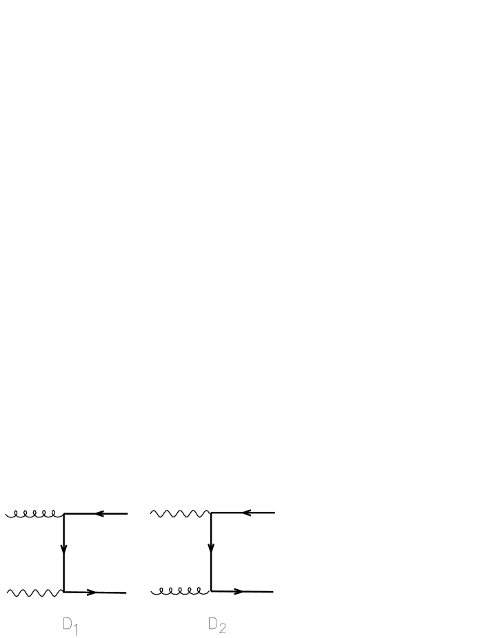
Figure 1: Diagrams for the $g\gamma$ Born amplitudes.

In the case of $S$-wave production we can set $Q=\overline{Q}=P/2$, and we get

$$\left(A^{[8]}_{\rm soft}\right)_{q=0} = {igf^{bca}\over\sqrt{2}}\left[{P\epsilon_{c}\over Pk}-{a\epsilon_{c}\over ak}\right]\,D_{12}\,.$$ (25)

In the case of ${}^{3}P$-waves we also need the derivative of the decay amplitude with respect to the relative momentum of the quark and antiquark. In the soft-gluon limit, we obtain:

$$\left({dA^{[8]}_{\rm soft}\over dq_{\alpha}}\right)_{q=0}\;=\;g{\sqrt{2}\over 2}\left\{if^{bca}\left[{P\epsilon_{c}\over Pk}-{a\epsilon_{c}\over ak}\right]{dD_{12}\over dq_{\alpha}}+d^{bca}\left[{\epsilon_{c}^{\alpha}\over Pk}-{k^{\alpha}\over(Pk)^{2}}(P\epsilon_{c})\right]D_{12}\right\}$$ (26)

Choosing a transverse gauge where $\epsilon_{c}\cdot P=0$, from eq. (9) and the previous two expressions it is straightforward to write

$${\cal A}_{{}^{3}P_{J}}\;=\;{\cal E}_{\alpha\beta}{igf^{bca}\over\sqrt{2}}\left[{P\epsilon_{c}\over Pk}-{a\epsilon_{c}\over ak}\right]{{{\mathrm{d}}}\over{{\mathrm{d}}q_{\beta}}}{\mathrm{T}r}\left.\left[{\cal C}\,{\mit\Pi}_{1}^{\alpha}{\cal A}_{\rm Born}\right]\right|_{q=0}\;+\;{gd^{bca}\over\sqrt{2}Pk}{\cal E}_{\alpha\beta}\epsilon_{c}^{\alpha}{\mathrm{T}r}\left.\left[{\cal C}\,{\mit\Pi}_{1}^{\alpha}{\cal A}_{\rm Born}\right]\right|_{q=0}\;.$$ (27)

The soft amplitude factorizes if the last term vanishes. This last term can be seen to be proportional to the amplitude for the production of a ${}^{3}S_{1}$ state, with an effective polarization $\epsilon_{\rm eff}$ given in terms of the polarizations of the soft gluon and of the ${}^{3}P_{J}$ state as follows:

$$\epsilon^{J}_{{\rm eff},\beta}\;=\;\epsilon_{c}^{\alpha}{\cal E}_{\alpha\beta}^{J}(P)\;.$$ (28)

If the average on the soft gluon $D-1$ spatial directions is taken, i.e.

$$\int{d\Omega^{D-1}_{k}\over\Omega^{D-1}}\sum_{\rm pol}\epsilon_{c}^{\alpha}\epsilon_{c}^{\beta*}={D-2\over D-1}\Pi_{\alpha\beta}(P)\;,$$ (29)

one can easily compute the sum over effective polarizations

$$\int{d\Omega^{D-1}_{k}\over\Omega^{D-1}}\sum_{\epsilon_{c}}\epsilon^{J}_{{\rm eff},\alpha}\epsilon^{J*}_{{\rm eff},\beta}=-N_{J}{D-2\over D-1}\Pi_{\alpha\beta}(P)\;,$$ (30)

where $N_{J}$ is the number of degrees of freedom of the ${}^{3}P_{J}$ state in $D$ dimensions. This shows that the last term in eq. (27), once squared and averaged on the directions of the outgoing gluon, is proportional to the amplitude of a ${}^{3}S_{1}$ state coupled to two gluons , which vanishes by $C$-parity. As a result we obtain the factorized expression:

$$\sum_{\rm col,pol}\;|\overline{A^{[8]}_{\rm soft}}|^{2}\;=\;\mbox{$C_{A}$}g^{2}\left[{2aP\over(ak)(Pk)}-{M^{2}\over(Pk)^{2}}\right]\sum_{\rm col,pol}\;|\overline{A^{[8]}_{\rm Born}}|^{2}$$ (31)

The amplitudes for $\gamma q\to{\cal{Q}}q$ are IR finite, and there is no need to study their soft behaviour for our applications.

3.2 Kinematics and factorization of soft and collinear singularities

The kinematics of the process $k+p_{1}\to P+p_{2}$, where $P$ is the momentum of the heavy quark pair, $k$ the momentum of the photon and $p_{i}$ are the momenta of the massless partons, can be described in terms of the standard Mandelstam variables $s$, $t$ and $u$:

$$s = (k+p_{1})^{2}\;,$$ (32)

$$t = (p_{1}-p_{2})^{2}\;\equiv\;-{s\over 2}(1-x)(1-y)\;,$$ (33)

$$u = (k-p_{2})^{2}\;\equiv\;-{s\over 2}(1-x)(1+y)\;.$$ (34)

Here we introduced the Lorentz-invariant dimensionless variables $x=M^{2}/s$ and $y$ ($-1<y<1$), defined by the above equations. In the center-of-mass frame of the partonic collisions, the variable $y$ becomes the cosine of the scattering angle $\theta$. In terms of $x$ and $y$ the total partonic cross-section can be written in $D$ dimensions as follows:

$$\sigma\;=\;{1\over 2s}\int d\Phi_{(2)}(x,y)\;\mbox{${\cal{M}}$}(x,y)\;,$$ (35)

where $\mbox{${\cal{M}}$}=\overline{\sum}|A|^{2}$ is the spin- and colour-averaged matrix element squared in $D$ dimensions and $d\Phi_{(2)}(x,y)$ is the $D$-dimensional two-body phase space:

$$d\Phi_{(2)}(x,y)\;=\;{4^{\epsilon}\over K}\,\left({4\pi\over s}\right)^{\epsilon}\,\Gamma(1+\epsilon)\,{1\over 16\pi}\,(1-x)^{1-2\epsilon}\,(1-y^{2})^{-\epsilon}\,dy\;,$$ (36)

with

$$K=\Gamma(1+\epsilon)\,\Gamma(1-\epsilon)=1+\epsilon^{2}{\pi^{2}\over 6}+{\cal O}(\epsilon^{3})\;.$$ (37)

The soft and collinear singularities are associated to the vanishing of $t$ or $u$, which appear at most as single poles in the expression of ${\cal{M}}$. One can therefore introduce the finite, rescaled amplitude squared ${\overline{\cal{M}}}$:

$$\mbox{${\cal{M}}$}\;=\;{1\over ut}\,\mbox{${\overline{\cal{M}}}$}\;=\;{4\over s^{2}(1-x)^{2}(1-y^{2})}\,\mbox{${\overline{\cal{M}}}$}\;.$$ (38)

In terms of ${\overline{\cal{M}}}$, the partonic cross-sections read as follows:

$$\sigma(x)\;=\;{4C\over s^{2}}\,(1-x)^{-1-2\epsilon}\,\int_{-1}^{1}\,dy\,(1-y^{2})^{-1-\epsilon}\,\mbox{${\overline{\cal{M}}}$}(x,y)\,dy\;,$$ (39)

$$C\;=\;{4^{\epsilon}\over K}\,\left({4\pi\over s}\right)^{\epsilon}\,\Gamma(1+\epsilon)\,{1\over 32\pi s}\;.$$ (40)

Soft and collinear singularities are now all contained in the universal poles which develop as $x\to 1$ and $y^{2}\to 1$. The residues of these poles can be derived without an explicit calculation of the matrix elements, as they only depend on the universal structure of collinear and soft singularities. We will carry out an explicit evaluation of these residues in the next section.

4 Results

4.1 $g\gamma\to g{\cal{O}}^{[8]}$ processes

Figure 2: Diagrams for the real corrections to the $g\gamma$ channels. Permutations of outgoing gluons and/or reversal of fermion lines are always implied.

We start by considering the soft limit, $x\to 1$. The following distributional identity holds for small $\epsilon$:

$$(1-x)^{-1-2\epsilon}\;=\;-{\beta^{-4\epsilon}\over 2\epsilon}\delta(1-x)+\left({1\over 1-x}\right)_{\rho}\,-\,2\epsilon\left({\log(1-x)\over 1-x}\right)_{\rho}\,+\,{\cal{O}}(\epsilon^{2})\,$$ (41)

where $\rho=M^{2}/S_{\gamma h}$, $h$ being the initial state target hadron, and $\beta=\sqrt{1-\rho}$. The $\rho$-distributions are defined by:

$$\int_{\rho}^{1}\,dx\;\left[d(x)\right]_{\rho}t(x)\;=\;\int_{\rho}^{1}\,dx\;d(x)\;\left[t(x)-t(1)\right]\;.$$ (42)

We can therefore write, with obvious notation,

$$\sigma(x)\;=\;\sigma_{x=1}+\sigma_{x\neq 1}\;.$$ (43)

The first term on the right-hand side is given by the following expression:

$$\sigma_{x=1}\;=\;-{4C\over M^{4}}\,{\tau^{-4\epsilon}\over 2\epsilon}\,\delta(1-x)\,\int_{-1}^{1}\,dy\,(1-y^{2})^{-1-\epsilon}\,\mbox{${\overline{\cal{M}}}$}(x=1,y)\;.$$ (44)

The $x\to 1$ limit of ${\overline{\cal{M}}}$ can be easily derived from eq. (31):

$$\mbox{${\overline{\cal{M}}}$}(x,y) \stackrel{{\scriptstyle x\to 1}}{{\longrightarrow}} s\,g^{2}\,\mbox{$C_{A}$}\,(1-y)^{2}\mbox{${\cal{M}}_{\rm Born}$}\;,$$ (45)

where ${\cal{M}}_{\rm Born}$ is the $D$-dimensional Born amplitude squared for the  $\gamma g\to{\cal{O}}^{[8]}$ process, which is independent of $y$. The integration over $y$ of eq. (44) is elementary, and leads to the following result:

$$\sigma_{x=1}\;=\;\left({4\pi\mu^{2}\over s}\right)^{\epsilon}{\Gamma(1+\epsilon)\,\tau^{-4\epsilon}\over 2\epsilon^{2}}\,H\,\mbox{$C_{A}$}\,{\mbox{$\alpha_{s}$}\over\pi}\,\mbox{$\sigma_{\rm Born}$}\;,$$ (46)

where $\alpha_{s}$ is related to the $D$-dimensional bare coupling $\alpha_{s}^{(b)}$ and to the renormalization scale $\mu$ by $\mbox{$\alpha_{s}$}\mu^{2\epsilon}=\mbox{$\alpha_{s}^{(b)}$}=g^{2}/4\pi$. $H$ is defined by

$$H\;=\;{\Gamma(2-\epsilon)\over\Gamma(1+\epsilon)\Gamma(2-2\epsilon)}\;=\;1+\epsilon+2\epsilon^{2}-{\pi^{2}\over 3}\epsilon^{2}+{\cal O}(\epsilon^{3})\;,$$ (47)

and $\sigma_{\rm Born}$ is the $D$-dimensional Born cross-section:

$$\mbox{$\sigma_{\rm Born}$}\;=\;\pi/M^{4}\mbox{${\cal{M}}_{\rm Born}$}\delta(1-x)\;\equiv\;\mbox{$\sigma_{0}$}\delta(1-x)\;.$$ (48)

The collinear singularities remaining in $\sigma_{x\neq 1}$ can be factored out by using the following distributional identity:

$$(1-y^{2})^{-1-\epsilon}\;=\;-\left[\delta(1-y)+\delta(1+y)\right]{4^{-\epsilon}\over 2\epsilon}+{1\over 2}\left[\left({1\over 1-y}\right)_{+}+\left({1\over 1+y}\right)_{+}\right]+{\cal O}(\epsilon)\;,$$ (49)

where the distributions on the right-hand side are defined by:

$$\int_{-1}^{1}\,dy\,\left({1\over 1\pm y}\right)_{+}t(y)\;=\;\int_{-1}^{1}\,dy\,{1\over 1\pm y}\left[t(y)-t(\mp 1)\right]\;.$$ (50)

The contribution $\sigma_{x\neq 1}$ can then be split into two terms:

$$\sigma_{x\neq 1}\;=\;\sigma_{y=1}+\sigma_{\rm finite}\;.$$ (51)

The term $\sigma_{\rm finite}$ has no residual divergences, and is given by the following expression:

$$\sigma_{\rm finite}\;=\;{2C\over s^{2}}\left({1\over 1-x}\right)_{\rho}\,\int_{-1}^{1}\,dy\,\left[\left({1\over 1-y}\right)_{+}+\left({1\over 1+y}\right)\right]\,\,\mbox{${\overline{\cal{M}}}$}(x,y)\;.$$ (52)

We removed the $+$ from the $1/(1+y)_{+}$ distribution because no collinear singularity can arise from the emission of the gluon collinear to the photon, and $\mbox{${\overline{\cal{M}}}$}(x,-1)=0$. $\sigma_{\rm finite}$ explicitly depends on the nature of the quarkonium state produced. For processes whose Born contribution vanishes, this is the only non zero term. $\sigma_{y=1}$ is given by:

$$\sigma_{y=1}\;=\;-{4C\over s^{2}}\,{4^{-\epsilon}\over 2\epsilon}\,\left[\left({1\over 1-x}\right)_{+}-2\epsilon\left({\log(1-x)\over 1-x}\right)_{+}\right]\,\mbox{${\overline{\cal{M}}}$}(x,y=1)\;.$$ (53)

The limit for $y\to 1$ of $\mbox{${\overline{\cal{M}}}$}(x,y)$ is universal, thanks to the factorization of collinear singularities:

$$\mbox{${\overline{\cal{M}}}$}(x,y)\stackrel{{\scriptstyle y\to 1}}{{\longrightarrow}}8\pi\,s\,\mbox{$\alpha_{s}^{(b)}$}P_{gg}(x){1-x\over x}\mbox{${\cal{M}}_{\rm Born}$}\;.$$ (54)

Using this relation we get:

$$\sigma_{y=1}\;=\;-{1\over\bar{\epsilon}}\,\left({\mu^{2}\over s}\right)^{\epsilon}\,{\mbox{$\alpha_{s}$}\over 2\pi}\,P_{gg}(x)\,(1-x)x\,\mbox{$\sigma_{0}$}\,\left[\left({1\over 1-x}\right)_{+}-2\epsilon\left({\log(1-x)\over 1-x}\right)_{+}\right]\;,$$ (55)

with

$$P_{gg}(x)=2\mbox{$C_{A}$}\left[{x\over 1-x}+{1-x\over x}+x(1-x)\right]\,.$$ (56)

and

$${1\over\bar{\epsilon}}\;=\;{1\over\epsilon}-\gamma_{\rm E}+\log(4\pi)\;,$$ (57)

The collinear poles take the form dictated by the factorization theorem. According to this the partonic cross-section can be written as:

$${\rm d}\sigma_{\gamma j}(p_{\gamma},p_{h}) = \sum_{l}{\rm d}\hat{\sigma}_{\gamma l}(p_{\gamma},xp_{h})\Gamma_{lj}(x){\rm d}x\;,$$ (58)

$$\Gamma_{ij}(x) = \delta_{ij}\delta(1-x)\;-\;{1\over\bar{\epsilon}}\,{\mbox{$\alpha_{s}$}\over 2\pi}\left({\mu^{2}\over\mbox{$\mu^{2}_{\rm F}$}}\right)^{\epsilon}{\cal P}_{ij}(x)\;+\;K_{ij}(x)\;,$$ (59)

where ${\rm d}\hat{\sigma}$ is free of collinear singularities as $\epsilon\to 0$. Here we allowed the factorization scale $\mu_{\rm F}$ to differ from the renormalization scale $\mu$. The functions ${\cal P}_{ij}(x)$ are the $D=4$ Altarelli-Parisi splitting kernels, collected in Appendix A, and the factors $K_{ij}$ are arbitrary functions, defining the factorization scheme. In this paper we adopt the $\overline{\rm MS}$  factorization, in which $K_{ij}(x)=0$ for all $i,j$. For the definition of $K_{ij}(x)$ in the DIS scheme, see for example ref. [28].

Figure 3: Diagrams for the $\gamma q$ channels. Reversal of fermion lines is always implied.

Expanding eq. (58) order-by-order in $\alpha_{s}$, we extract the counter-term $\sigma^{(c)}_{y=1}$, defined by:

$$\sigma^{(c)}_{y=1}\;=\;{1\over\bar{\epsilon}}\,{\mbox{$\alpha_{s}$}\over 2\pi}\left({\mu^{2}\over\mbox{$\mu^{2}_{\rm F}$}}\right)^{\epsilon}\,{\cal{P}}_{gg}({x}\,)x\mbox{$\sigma_{0}$}\;,$$ (60)

with

$${\cal P}_{gg}(x)=2\mbox{$C_{A}$}\left[{x\over(1-x)_{\rho}}+{1-x\over x}+x(1-x)\right]+\left(\mbox{$b_{0}$}+4\mbox{$C_{A}$}\log\beta\right)\delta(1-x)\,.$$ (61)

Putting all pieces together, we come to the final result for the real-emission cross-section:

$$\sigma^{H}[g\gamma\to{\cal{Q}}^{[8]}g](x) = {\mbox{$\alpha_{s}$}\over 2\pi}\sigma_{0}^{H}[g\gamma\to{\cal{Q}}^{[8]}]$$ (62)

$$\times \left\{f_{\epsilon}(s)\left[\mbox{$C_{A}$}\left({1\over\mbox{$\epsilon$}^{2}}+{17\over 6\mbox{$\epsilon$}}+2-{\pi^{2}\over 3}-4\log\tau+8\log^{2}\tau\right)-{2\over 3\mbox{$\epsilon$}}\mbox{$n_{f}$}\mbox{$T_{F}$}\right]\delta(1-x)+\right.$$

$$+ \left.\left[x{\cal P}_{gg}(x)\log{s\over\mbox{$\mu^{2}_{\rm F}$}}+2x(1-x)P_{gg}(x)\left({\log(1-x)\over 1-x}\right)_{\rho}+\left({1\over 1-x}\right)_{\rho}f_{\gamma g}[{\cal{Q}}^{[8]}](x)\right]\right\}$$

$$[{\cal{Q}}^{[8]}={{}^{1}S_{0}^{[8]}},{{}^{3}P_{0}^{[8]}},{{}^{3}P_{2}^{[8]}}]\;,$$

where $f_{\epsilon}(s)$ is defined in Appendix A and $\sigma_{0}^{H}[\gamma g\to{\cal{Q}}^{[8]}]$ is the $D$-dimensional, Born-level partonic cross-section for the production of the quarkonium state $H$ via the ${\cal{Q}}^{[8]}$ intermediate state, after removal of the $\delta(1-x)$ term (see eq. (48)). The finite functions $f_{\gamma g}(x)$, obtained from the explicit evaluation of eq. (52), are collected in Appendix B.

4.2 $q\gamma\to q{\cal{Q}}^{[8]}$ processes

The Born-level processes $q\gamma\to{\cal{Q}}^{[8]}$ identically vanish. As a result IR divergences at $O(\mbox{$\alpha_{s}^{2}$}\mbox{$\alpha_{{\mathrm{\tiny}em}}$})$ and virtual corrections are not present. The only possible singularities appearing at this order come from the emission of the final-state quark collinear to the initial-state one or to the photon.. The behaviour of the amplitude (fig. 3(a)) for ${\cal{Q}}^{[8]}={{}^{1}S_{0}^{[8]}},{{}^{3}P_{0}^{[8]}},{{}^{3}P_{2}^{[8]}}$ in the $y\to 1$ collinear limit is again controlled by the Altarelli-Parisi splitting functions:

$$\mbox{${\overline{\cal{M}}}$}(x,y)\stackrel{{\scriptstyle y\to 1}}{{\longrightarrow}}8\pi\,s\,\mbox{$\alpha_{s}^{(b)}$}P_{gq}(x){1-x\over x}\mbox{${\cal{M}}_{\rm Born}$}\;.$$ (63)

In analogy to the $\gamma g$ case, one introduces the following counter-term in the $\overline{\rm MS}$  scheme:

$$\sigma^{(c)}_{y=1}\;=\;{1\over\bar{\epsilon}}\,{\mbox{$\alpha_{s}$}\over 2\pi}\left({\mu^{2}\over\mbox{$\mu^{2}_{\rm F}$}}\right)^{\epsilon}\,{\cal{P}}_{gq}({x}\,)x\mbox{$\sigma_{0}$}\;,$$ (64)

where ${\cal{P}}_{gq}({x}\$)is defined in Appendix A.

Following a procedure analogous to the one detailed in the case of $\gamma g$ production, we find the following result:

$$\sigma^{H}[\gamma\,q\to{\cal{Q}}^{[8]}\,q](x) = {\mbox{$\alpha_{s}$}\over\pi}\sigma_{0}^{H}[\gamma g\to{\cal{Q}}^{[8]}]\times$$ (65)

$$\left\{\left[{x\over 2}P_{gq}(x)\log{s(1-x)^{2}\over\mbox{$\mu^{2}_{\rm F}$}}+\mbox{$C_{F}$}{x^{2}\over 2}\right]+f_{\gamma q}[{\cal{Q}}^{[8]}](x)\right\}\,,$$

$$[{\cal{Q}}^{[8]}={{}^{1}S_{0}^{[8]}},{{}^{3}P_{0}^{[8]}},{{}^{3}P_{2}^{[8]}}]\;,$$

where the functions $f_{\gamma q}(x)$ are collected in Appendix B, together with the result for ${{}^{3}P_{1}}$ production, for which no collinear singularity is present to start with.

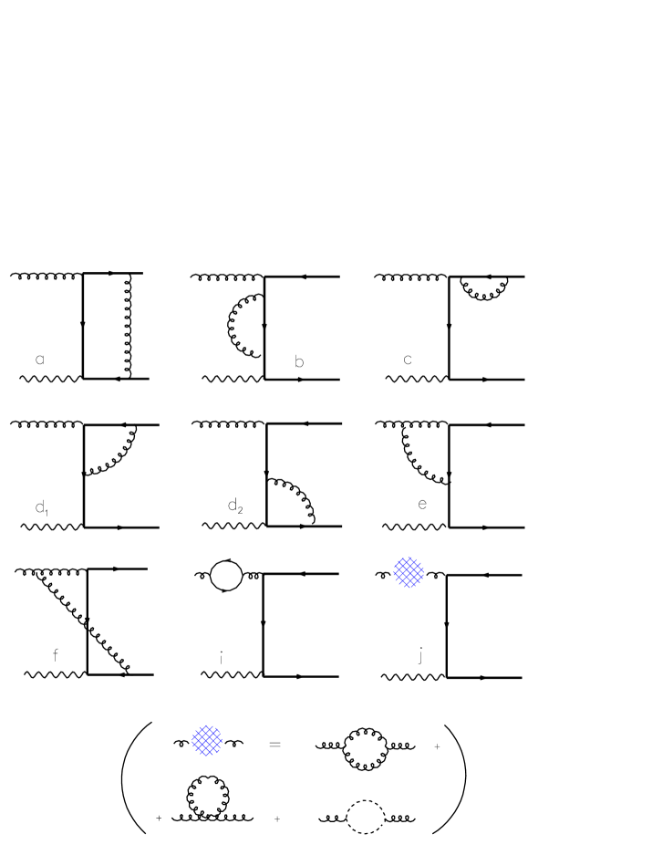
Figure 4: Feynman diagrams contributing to the one-loop corrections to the processes $g\gamma\to Q\overline{Q}[^{3}P_{0}^{[8]}]$, $g\gamma\to Q\overline{Q}[^{3}P_{2}^{[8]}]$ and $g\gamma\to Q\overline{Q}[^{1}S_{0}^{[8]}]$.

For ${{}^{3}S_{1}^{[8]}}$ production only the diagram in fig. 3(b) gives a non vanishing contribution. In the $y\to 1$ collinear limit we have:

$$\mbox{${\overline{\cal{M}}}$}(x,y)\stackrel{{\scriptstyle y\to 1}}{{\longrightarrow}}8\pi\,s\,\mbox{$\alpha^{(b)}_{{\mathrm{\tiny}em}}$}e_{Q}^{2}P_{q\gamma}(x){1-x\over x}\mbox{${\cal{M}}_{\rm Born}$}\;.$$ (66)

where ${\cal{M}}_{\rm Born}$ is the Born amplitude for the process $\mbox{$q\overline{q}$}\to{{}^{3}S_{1}^{[8]}}$ and $P_{q\gamma}(x)$ is the Altarelli-Parisi photon-splitting function in $D$ dimensions. Introducing the following counter-term in the $\overline{\rm MS}$  scheme:

$$\sigma^{(c)}_{y=1}\;=\;{1\over\bar{\epsilon}}\,{\mbox{$\alpha_{{\mathrm{\tiny}em}}$}e_{Q}^{2}\over 2\pi}\left({\mu^{2}\over\mbox{$\mu_{\gamma}$}^{2}}\right)^{\epsilon}\,{\cal{P}}_{q\gamma}({x}\,)x\mbox{$\sigma_{0}$}\;,$$ (67)

where ${\cal{P}}_{q\gamma}(x)\$ is defined in Appendix A, we can write the following partonic cross-section:

$$\mbox{$\sigma^{H}$}[\,\gamma\,q\to{{}^{3}S_{1}^{[8]}}\,q](x) = {\mbox{$\alpha_{{\mathrm{\tiny}em}}$}\mbox{$e^{2}_{Q}$ }\over\pi}\mbox{$\sigma_{0}^{H}$}[\mbox{$q\overline{q}$}\to{{}^{3}S_{1}^{[8]}}]$$ (68)

$$\times\left\{\left[{x\over 2}P_{q\gamma}(x)\log{s(1-x)^{2}\over\mu_{\gamma}^{2}}+\mbox{$D_{F}$}x^{2}(1-x)\right]+f_{\gamma q}[{{}^{3}S_{1}^{[8]}}](x)\right\}$$

Having absorbed the collinear $\gamma\to q$ divergence in the photon structure function, the total cross-section will now include a piece proportional to the resolved component of the photon (see, e.g. , ref. [29, 18]):

$${\rm d}\sigma_{\gamma\,h}(p_{1},p_{h}) = \sum_{i}{\rm d}\hat{\sigma}_{\gamma i}(xS,\mbox{$\mu_{\rm F}$},\mbox{$\mu_{\gamma}$})F_{i\,h}(x,\mbox{$\mu_{\rm F}$}){\rm d}x$$ (69)

$$+\sum_{k,l}{\rm d}\hat{\sigma}_{kl}(x_{1}p_{\gamma},x_{2}p_{h},\mbox{$\mu_{\rm F}$})F_{k\gamma}(x_{1},\mbox{$\mu_{\gamma}$})F_{lh}(x_{2},\mbox{$\mu_{\rm F}$}){\rm d}x_{1}{\rm d}x_{2}\;,$$

where $F_{k\gamma}(x,\mbox{$\mu_{\gamma}$})$ is the density of the parton $k$ in the photon, and $F_{kh}(x,\mbox{$\mu_{\rm F}$})$ is the density of the parton $k$ in the hadron $h$. The full $O(\alpha_{s}^{3})$ expression for the parton-parton ${{}^{3}S_{1}^{[8]}}$ cross-sections to be used in the resolved-photon contribution to the above equation can be found in [21].

Diag.	${\cal D}_{k}$	$f_{k}^{(8)}$
a	${\pi^{2}\over 2v}+{1\over\mbox{$\epsilon$}}-2+2\log 2$	$C_{F}-{1\over 2}C_{A}$
b	$-{1\over 2\mbox{$\epsilon_{\!\!\mbox{ \tiny{UV} }}$}}-1+3\log 2$	$C_{F}$
c	$-{1\over 2\mbox{$\epsilon_{\!\!\mbox{ \tiny{UV} }}$}}-{1\over\mbox{$\epsilon$}}-2-3\log 2$	$C_{F}$
${\rm d}_{1}$	${1\over 2\mbox{$\epsilon_{\!\!\mbox{ \tiny{UV} }}$}}-\log 2+{\pi^{2}\over 8}$	$C_{F}$
${\rm d}_{2}$	${1\over 2\mbox{$\epsilon_{\!\!\mbox{ \tiny{UV} }}$}}-\log 2+{\pi^{2}\over 8}$	$C_{F}-{1\over 2}C_{A}$
e	$+{3\over 2\mbox{$\epsilon_{\!\!\mbox{ \tiny{UV} }}$}}-{1\over 2\mbox{$\epsilon$}^{2}}-{1\over 2\mbox{$\epsilon$}}+2-\log 2+{\pi^{2}\over 12}$	${1\over 2}$$C_{A}$
f	$-{1\over 2\mbox{$\epsilon$}^{2}}-{1\over 2\mbox{$\epsilon$}}-1+2\log 2+{5\over 24}\pi^{2}$	${1\over 2}\mbox{$C_{A}$}$
i	${5\over 12\mbox{$\epsilon_{\!\!\mbox{ \tiny{UV} }}$}}-{5\over 12\mbox{$\epsilon$}}$	$C_{A}$
j	$\left(-{1\over 3\mbox{$\epsilon_{\!\!\mbox{ \tiny{UV} }}$}}+{1\over 3\mbox{$\epsilon$}}\right)\mbox{$n_{f}$}$	$T_{F}$

Table 1: “Diagrammatic” partial virtual QCD corrections to the processes $g\gamma\to[^{1}S_{0}^{[8]}]$ (diagram multiplicities are included)

Diag.	${\cal D}_{k}$	$f_{k}^{(8)}$
a	${\pi^{2}\over 2v}+{1\over\mbox{$\epsilon$}}-{4\over 9}+{32\over 9}\log 2+{\pi^{2}\over 12}$	$C_{F}-{1\over 2}C_{A}$
b	$-{1\over 2\mbox{$\epsilon_{\!\!\mbox{ \tiny{UV} }}$}}-{13\over 9}+{5\over 9}\log 2$	$C_{F}$
c	$-{1\over 2\mbox{$\epsilon_{\!\!\mbox{ \tiny{UV} }}$}}-{1\over\mbox{$\epsilon$}}-2-3\log 2$	$C_{F}$
${\rm d}_{1}$	${1\over 2\mbox{$\epsilon_{\!\!\mbox{ \tiny{UV} }}$}}+{7\over 9}-{5\over 9}\log 2+{\pi^{2}\over 12}$	$C_{F}$
${\rm d}_{2}$	${1\over 2\mbox{$\epsilon_{\!\!\mbox{ \tiny{UV} }}$}}+{7\over 9}-{5\over 9}\log 2+{\pi^{2}\over 12}$	$C_{F}-{1\over 2}C_{A}$
e	${3\over 2\mbox{$\epsilon_{\!\!\mbox{ \tiny{UV} }}$}}-{1\over 3\mbox{$\epsilon$}^{2}}-{10\over 9\mbox{$\epsilon$}}+{11\over 6}-{1\over 3}\log 2+{\pi^{2}\over 18}$	${1\over 2}$$C_{A}$
f	$-{2\over 3\mbox{$\epsilon$}^{2}}+{1\over 9\mbox{$\epsilon$}}-{1\over 2}+{10\over 3}\log 2+{5\over 18}\pi^{2}$	${1\over 2}$$C_{A}$
i	${5\over 12\mbox{$\epsilon_{\!\!\mbox{ \tiny{UV} }}$}}-{5\over 12\mbox{$\epsilon$}}$	$C_{A}$
j	$\left(-{1\over 3\mbox{$\epsilon_{\!\!\mbox{ \tiny{UV} }}$}}+{1\over 3\mbox{$\epsilon$}}\right)\mbox{$n_{f}$}$	$T_{F}$

Table 2: “Diagrammatic” partial virtual QCD corrections to the processes $g\gamma~{}\to~{}[^{3}P_{0}^{[8]}]$ (diagram multiplicities are included).

Diag.	${\cal D}_{k}$	$f_{k}^{(8)}$
a	${\pi^{2}\over 2v}+{1\over\mbox{$\epsilon$}}-{5\over 3}+{7\over 3}\log 2+{\pi^{2}\over 8}$	$C_{F}-{1\over 2}C_{A}$
b	$-{1\over 2\mbox{$\epsilon_{\!\!\mbox{ \tiny{UV} }}$}}-{1\over 6}+{11\over 6}\log 2$	$C_{F}$
c	$-{1\over 2\mbox{$\epsilon_{\!\!\mbox{ \tiny{UV} }}$}}-{1\over\mbox{$\epsilon$}}-2-3\log 2$	$C_{F}$
${\rm d}_{1}$	${1\over 2\mbox{$\epsilon_{\!\!\mbox{ \tiny{UV} }}$}}-{1\over 12}-{7\over 12}\log 2-{\pi^{2}\over 16}$	$C_{F}$
${\rm d}_{2}$	${1\over 2\mbox{$\epsilon_{\!\!\mbox{ \tiny{UV} }}$}}-{1\over 12}-{7\over 12}\log 2-{\pi^{2}\over 16}$	$C_{F}-{1\over 2}C_{A}$
e	${3\over 2\mbox{$\epsilon_{\!\!\mbox{ \tiny{UV} }}$}}-{3\over 16\mbox{$\epsilon$}^{2}}-{17\over 32\mbox{$\epsilon$}}+{59\over 192}+{\pi^{2}\over 32}$	${1\over 2}$$C_{A}$
f	$-{13\over 16\mbox{$\epsilon$}^{2}}-{15\over 32\mbox{$\epsilon$}}-{107\over 192}+{11\over 4}\log 2+{67\over 96}\pi^{2}$	${1\over 2}\mbox{$C_{A}$}$
i	${5\over 12\mbox{$\epsilon_{\!\!\mbox{ \tiny{UV} }}$}}-{5\over 12\mbox{$\epsilon$}}$	$C_{A}$
j	$\left(-{1\over 3\mbox{$\epsilon_{\!\!\mbox{ \tiny{UV} }}$}}+{1\over 3\mbox{$\epsilon$}}\right)\mbox{$n_{f}$}$	$T_{F}$

Table 3: “Diagrammatic” partial virtual QCD corrections to the processes $g\gamma\to[^{3}P_{2}^{[8]}]$ (diagram multiplicities are included).

4.3 Virtual corrections

We present in this section the results of the calculation of the 1-loop diagrams necessary for the evaluation of the virtual corrections to the production matrix elements. These results can be obtained in a straightforward way from the calculation of the virtual corrections to 1-loop hadroproduction, presented in ref. [21]. We shall therefore limit ourselves to presenting the final answers. The relevant Feynman diagrams are shown in figures  4, and the results are given diagram by diagram in tables 1, 2, 3. In these tables we report the contribution of each diagram $k$, indicating separately the colour factors $f_{k}$. The expressions ${\cal D}_{k}$ appearing in the tables are defined by the following equation:

$$\sigma_{V}^{H}[ij\to{\cal{Q}}]={\mbox{$\alpha_{s}$}\mu^{2\mbox{$\epsilon$}}\over\pi}\sigma_{0}^{H}[ij\to{\cal{Q}}]\,f_{\epsilon}(s)\sum_{k}{\cal D}_{k}f_{k}\,\delta(1-x).$$ (70)

where the sum extends over the set of diagrams and $f_{\epsilon}(s)$ is defined in Appendix A.

The singularity structure of the virtual corrections is dictated by the renormalization properties of the theory, by the universal form of the Coulomb limit, and by requirement that soft and collinear singularities cancel against the real corrections evaluated above. The form of the virtual corrections to the cross-section is therefore the following:

$$\sigma^{(V)}\;=\;\sigma_{0}{\mbox{$\alpha_{s}$}\over 2\pi}f_{\epsilon}(s)\times\left\{{b_{0}\over\epsilon_{\rm UV}}+(\mbox{$C_{F}-{1\over 2}C_{A}$}){\pi^{2}\over v}-\mbox{$C_{A}$}\left({1\over\epsilon_{\rm IR}^{2}}+{17\over 6\epsilon_{\rm IR}}\right)+{2\over 3\epsilon_{\rm IR}}\mbox{$n_{f}$}\mbox{$T_{F}$}+2\,D^{[8]}_{{\cal{O}}}\right\}\;,$$ (71)

where we explicitly labelled the $\epsilon$’s to indicate their origin, and where all of the state dependence is included in the finite factor $D_{{\cal{Q}}}$. The quark-antiquark relative velocity $2v$ and $b_{0}$ are defined in Appendix A. $n_{f}$ is the number of flavours lighter than the heavy, bound one.

Summing the contribution of all diagrams, we obtain the following results for the colour-octet coefficients $D_{{\cal{Q}}}^{[8]}$ :

$$D^{[8]}_{{{}^{1}S_{0}}}\;=\;\;\mbox{$C_{F}$}\left(-5+{\pi^{2}\over 4}\right)+\mbox{$C_{A}$}\left({3\over 2}+{\pi^{2}\over 12}\right)$$ (72)

$$D^{[8]}_{{{}^{3}P_{0}}}\;=\;\mbox{$C_{F}$}\left(-{7\over 3}+{\pi^{2}\over 4}\right)+\mbox{$C_{A}$}\left({1\over 2}+{\pi^{2}\over 12}\right)$$ (73)

$$D^{[8]}_{{{}^{3}P_{2}}}\;=\;-4\mbox{$C_{F}$}+\mbox{$C_{A}$}\left({3\over 4}+{\log 2\over 2}+{\pi^{2}\over 3}\right)\;.$$ (74)

The final results for the finite sums of real plus virtual corrections are collected in Appendix B.

5 Phenomenology

In this section we study some of the properties of the higher-order corrections calculated in this paper, and their effect on typical Born-level predictions. A more thorough phenomenological study including a comparison to currently available data and fits to the non-perturbative parameters will be presented elsewhere.

Figure 5: Born and NLO total photoproduction cross-sections as a function of the photon beam energy.

Figure 6: Born and NLO total photoproduction cross-sections as a function of the $\gamma$p CM energy.

To start with, we show in fig. 5 the comparison between Born and NLO total photoproduction cross-sections as a function of the photon beam energy, in the energy range of fixed-target experiments. Here and in the following, we concentrate on the colour-octet contributions of ${{}^{1}S_{0}}$, ${{}^{3}P_{0}}$ and ${{}^{3}P_{2}}$ states, which are by far the dominant processes. We fix $m_{c}=1.5$ GeV and we take, for the sake of definiteness [8], $\mbox{$\langle 0|{\cal O}_{8}^{\psi}(^{1}S_{0})|0\rangle$}=0.01$ GeV^-3 and $\mbox{$\langle 0|{\cal O}_{8}^{\psi}(^{3}P_{0})|0\rangle$}/m_{c}^{2}=0.01$ GeV^-5, with $\mbox{$\langle 0|{\cal O}_{8}^{\psi}(^{3}P_{J})|0\rangle$}=(2J+1)\mbox{$\langle 0|{\cal O}_{8}^{\psi}(^{3}P_{0})|0\rangle$}$.

Figure 7: Separate contributions from Born, $O(\alpha_{s}^{2}\mbox{$\alpha_{{\mathrm{\tiny}em}}$})$ $\gamma g$ and $O(\alpha_{s}^{2}\mbox{$\alpha_{{\mathrm{\tiny}em}}$})$ $\gamma q$ processes to total photoproduction cross-sections as a function of the photon beam energy.

Figure 8: Separate contributions from Born, $O(\alpha_{s}^{2}\mbox{$\alpha_{{\mathrm{\tiny}em}}$})$ $\gamma g$ and $O(\alpha_{s}^{2}\mbox{$\alpha_{{\mathrm{\tiny}em}}$})$ $\gamma q$ processes to total photoproduction cross-sections as a function of the $\gamma p$ CM energy.

Figure 9: Ratios of the ${{}^{3}P_{J}^{[8]}}$ to ${{}^{1}S_{0}^{[8]}}$ production rates at NLO, normalized to a common choice of non-perturbative matrix elements, as a function of the photon beam energy. The Born-level predictions for these ratios are equal to 3 and 4 for the ratios of ${{}^{3}P_{0}^{[8]}}/{{}^{1}S_{0}^{[8]}}$ and ${{}^{3}P_{2}^{[8]}}/{{}^{1}S_{0}^{[8]}}$, respectively.

The scale dependence of the results is displayed by the curves relative to the scale choices ${\mbox{$\mu_{\rm R}$}}=\mbox{$\mu_{\rm F}$}=aM$, with $a=1/2,1$ and 2. We chose the MRSA set of parton densities [30], including the low-$Q^{2}$ corrections [31] necessary to evaluate consistently the cross-sections when using the smaller choice of scales, $\mbox{$\mu_{\rm F}$}=M/2$. These low-$Q^{2}$ corrections are essential to properly estimate the true scale-dependence of the calculation. Similar curves for the energy range typical of the HERA collider (given as a function of $\sqrt{S_{\gamma p}}$, the $\gamma p$ CM energy), are shown in fig. 6. Notice the significant improvement in the scale dependence when the NLO corrections are included. This improvement is less remarkable at low energies. The reason for this is that the $q\gamma\to q{\cal{Q}}$ is particularly important at low energies. This process first appears at $O(\alpha_{s}^{2}\mbox{$\alpha_{{\mathrm{\tiny}em}}$})$, and is therefore calculated at LO only. Its contribution becomes less important at high energies, where the gluon-initiated process dominates, and the $O(\alpha_{s}^{2}\mbox{$\alpha_{{\mathrm{\tiny}em}}$})$ calculations are therefore genuinely NLO. As a result of this, the $K$-factor (defined as the ratio of the $\mbox{$O(\alpha_{s}^{2}\mbox{$\alpha_{{\mathrm{\tiny}em}}$})$}/$Born results) is larger at low energy (exceeding a factor of 2) than at high energies.

The relative importance of the gluon and quark processes is displayed in figs. 7 and 8, for the fixed-target and collider-energy ranges, respectively. Notice that the contribution of the $q\gamma$ channel is always negative. This is the result of the subtraction of the mass singularities present in the $q\gamma\to q{\cal{Q}}$ channel when the final-state quark is emitted collinear to the beam. The collinear singularities are absorbed in the gluon parton density at NLO, as explained in the previous sections. The net result of this subtraction, in the $\overline{\rm MS}$  scheme, is a negative contribution of the factorized $q\gamma$ process.

An important element in previous Born-level extractions [8, 9] of the non-perturbative colour-octet parameters from the fit to fixed-target and HERA data is the set of relations:

$$\sigma^{\psi}[{{}^{3}P_{0}^{[8]}}]\;=\;3{m_{c}^{2}\mbox{$\langle 0|{\cal O}_{8}^{\psi}(^{3}P_{0})|0\rangle$}\over\mbox{$\langle 0|{\cal O}_{8}^{\psi}(^{1}S_{0})|0\rangle$}}\sigma^{\psi}[{{}^{1}S_{0}^{[8]}}]\quad,\quad\sigma^{\psi}[{{}^{3}P_{2}^{[8]}}]\;=\;4{m_{c}^{2}\mbox{$\langle 0|{\cal O}_{8}^{\psi}(^{3}P_{0})|0\rangle$}\over\mbox{$\langle 0|{\cal O}_{8}^{\psi}(^{1}S_{0})|0\rangle$}}\sigma^{\psi}[{{}^{1}S_{0}^{[8]}}]\;.$$ (75)

In these relations we assumed, as usual, $\mbox{$\langle 0|{\cal O}_{8}^{\psi}(^{3}P_{J})|0\rangle$}=(2J+1)\mbox{$\langle 0|{\cal O}_{8}^{\psi}(^{3}P_{0})|0\rangle$}$. As a result of these relations, one could use the following identity:

$$\sigma(\psi)=\Theta\;\hat{\sigma}[{{}^{1}S_{0}^{[8]}}]\;,\quad\quad\mbox{with }\quad\Theta=\mbox{$\langle 0|{\cal O}_{8}^{\psi}(^{1}S_{0})|0\rangle$}+7{\mbox{$\langle 0|{\cal O}_{8}^{\psi}(^{3}P_{0})|0\rangle$}\over m_{c}^{2}}\;.$$ (76)

The validity of these Born-level relations when the NLO corrections are included is studied in figs 9 and 10, which show the ratios of ${{}^{3}P_{J}^{[8]}}$ and ${{}^{1}S_{0}^{[8]}}$ production at NLO. As the figures indicate, the relation in eq. (76) holds at NLO to within 10%. Notice that the individual relative contributions of the ${{}^{3}P_{0}^{[8]}}$ and ${{}^{3}P_{2}^{[8]}}$ states can however change by up to 30% with respect to the Born-level prediction $\sigma[{{}^{3}P_{0}^{[8]}}]/\sigma[{{}^{3}P_{2}^{[8]}}]$ = 4/3.

Figure 10: Same as fig. 9, as a function of the $\gamma$p CM energy.

5.1 High-energy behaviour

While the current experiments only allow to study $\psi$ photoproduction up to CM energies of the order of few hundred GeV, it is interesting to consider the behaviour of the total cross-sections in the asymptotic regime. In this regime, interesting phenomena are expected to take place, because of the potentially large small-$x$ effects associated to the presence of diagrams with $t$-channel gluon exchange. Because of these contributions, the total partonic cross-sections tend to a constant limit when $x\to 0$. It is easy to see, in fact, that:

$$\mbox{$\sigma^{H}$}[\gamma\,i\to{\cal{Q}}i]\stackrel{{\scriptstyle x\to 0}}{{\to}}-\,\left({\mbox{$\alpha_{s}$}\over\pi}\right)\;Z_{i}\;Z_{{\cal{Q}}}\;\mbox{$\sigma_{0}^{H}$}[\gamma g\to{\cal{Q}}]\;,\quad(i=q,g)\;,$$ (77)

where

$$Z_{q}=\mbox{$C_{F}$}\quad,\quad Z_{g}=\mbox{$C_{A}$}\;,$$ (78)

and

$$Z_{{{}^{1}S_{0}^{[8]}}} = 1-\log({M^{2}\over\mbox{$\mu_{\rm F}$}^{2}})\;,$$ (79)

$$Z_{{{}^{3}P_{0}^{[8]}}} = {43\over 27}-\log({M^{2}\over\mbox{$\mu_{\rm F}$}^{2}})\;,$$ (80)

$$Z_{{{}^{3}P_{0}^{[8]}}} = {53\over 36}-\log({M^{2}\over\mbox{$\mu_{\rm F}$}^{2}})\;.$$ (81)

Notice that in the $x\to 0$ limit the ratio between the quark and gluon channels is equal to $\mbox{$C_{F}$}/\mbox{$C_{A}$}$, as expected. The factors for the $\gamma q$ channel are the same as those for the $gq$ channel [21]. The factors for the $gammag$ channel are half those for the $gg$ channel [21]. This is as expected, since in this last case the soft $t$-channel gluon can be radiated from either of the two initial state gluons. These results are trivial but useful cross-checks of our calculations.

Notice also that the small-$x$ partonic cross-sections tend to a negative value, unless the factorization scale is chosen to be very small. The large contribution coming from the small-$x$ region, and the large scale-dependence of the asymptotic $x\to 0$ limit, suggest that the NLO calculations should display a large dependence on the scale and on the shape of gluon densities at sufficiently high CM energies. A similar behaviour has already been observed in the NLO hadroproduction case [22].

To study this issue in more detail, we assume the gluon density to take, at a given scale $\mu_{\rm F}$, the form:

$$G(x)={1\over x^{1+\delta}}\quad,\quad 0<\delta<1\;.$$ (82)

The softer the gluon density ($\delta\to 0$), the more important the small-$x$ contributions will be. In the extreme case of $\delta=0$, it is easy to find the following result for the NLO/LO $K$-factors of the total production cross setions, exact up to order $\rho=M^{2}/S_{\gamma p}$:

$$K[{\cal{Q}}]\;=\;1+{\mbox{$\alpha_{s}$}\over\pi}\left[{1\over 2}A_{\rm tot}[{\cal{Q}}]+\mbox{$C_{A}$}k_{{\cal{Q}}}-{11\over 6}\mbox{$C_{A}$}\log({M^{2}\over\mbox{$\mu_{\rm F}$}^{2}})-\mbox{$C_{A}$}Z_{{\cal{Q}}}\log({1\over\rho})\right]$$ (83)

where the coefficients $A_{\rm tot}[{\cal{Q}}]$ are collected in Appendix B, the $Z_{{\cal{Q}}}$’s are given in eqs. (79)–(81) and

$$k_{{{}^{1}S_{0}^{[8]}}} = {25\over 3}-{13\over 24}\pi^{2}$$ (84)

$$k_{{{}^{3}P_{0}^{[8]}}} = {43\over 3}-{467\over 432}\pi^{2}$$ (85)

$$k_{{{}^{3}P_{2}^{[8]}}} = {595\over 48}-{1067\over 1152}\pi^{2}$$ (86)

Figure 11: High-energy behaviour of the $K$ factor for the $\gamma g$ process, using a gluon density $G(x)=1/x$, as a function of the $\gamma$p CM energy.

Figure 12: Small-$x$ behaviour of the gluon density at $\mbox{$\mu_{\rm F}$}=3$ GeV, for the MRSA [30] and CTEQ4M [32] fits. Arbitrary normalization.

As anticipated, large negative logarithmic terms arise. The scale dependence of the coefficient of the $\log\rho$ terms cannot be used to change the overall sign, since it is formally compensated by the scale dependence of the gluon density, which in the $\delta=0$ case is given by:

$${dG(\rho)\over d\log{\mbox{$\mu^{2}_{\rm F}$}}}={\mbox{$\alpha_{s}$}\over 2\pi}\;\int_{\rho}^{1}\;{dz\over z}\;P_{gg}(z)\;G(\rho/z,\mbox{$\mu_{\rm F}$})\sim{\mbox{$C_{A}$}\mbox{$\alpha_{s}$}\over\pi}G(\rho)\log{1\over\rho}.$$ (87)

The behaviour of these functions is shown in fig. 11. The $K$-factor becomes negative already for relatively small values of $\sqrt{S_{\gamma p}}$, making the NLO estimates unreliable.

Figure 13: High-energy behaviour of the $K$ factor for the $\gamma g$ process, using a gluon density $G(x)=1/x^{1+\delta}$, as a function of the $\gamma$p CM energy and for different values of $\delta$.

This result is not inconsistent with the nice behaviour of the cross-sections at $\sqrt{S_{\gamma p}}\sim 100$ GeV seen in fig. 6, since in that figure the results were obtained using the more realistic set of parton densities MRSA. Typical values of $\delta$ at $\mbox{$\mu_{\rm F}$}=3$ GeV for the current fits of the gluon densities [30, 32] are around $\delta=0.3$ (see fig. 12). The stability of the predictions in fact improves for $\delta>0$, when the contribution of the small-$x$ regime is suppressed. One can easily verify in fact that for $\delta\log(1/\rho)\gg 1$ the asymptotic behaviour of the $K$-factor is given by:

$$K[{\cal{Q}}]\stackrel{{\scriptstyle\rho\to 0}}{{\to}}1+{\mbox{$\alpha_{s}$}\over\pi}{1\over\delta}\left(Z_{{\cal{Q}}}+{\cal O}(\delta,\rho)\right)\;,$$ (88)

Depending on the value of $\delta$, the NLO correction can still be large and negative. Figure 13 shows the high-energy behaviour of the $K$-factor for the values $\delta=0.2$ and $\delta=0.4$ . As predicted by eq. (88), the $K$-factor tends to a constant.

6 Conclusions

We presented in this paper the first calculation of $O(\alpha_{s}^{2}\mbox{$\alpha_{{\mathrm{\tiny}em}}$})$ corrections to the total quarkonium photoproduction cross-sections. The calculations have been performed in the framework of the NRQCD approach to quarkonium production. As in the Born-level case, the production is dominated by colour-octet $Q\overline{Q}$ states. The contribution to the cross-sections from the NLO corrections is large at typical fixed-target energies (up to a factor of 2 increase over the Born results), and decreases at energies typical of the HERA collider. In this energy range the NLO corrections significantly improve the stability of the calculated rates under variations of the renormalization and factorization scales. For energies above few hundred GeV in the $\gamma p$ CM frame, large and negative small-$x$ contributions dominate the production rate, and make the NLO evaluation of the total cross-sections strongly dependend on the scale and shape of the gluon density, calling for the resummation of small-$x$ effects.

The calculations presented in this paper do not directly improve our knowledge of the quarkonium photoproduction at $\mbox{$p_{T}$}>0$, since production at $\mbox{$p_{T}$}>0$ is a process of $O(\alpha_{s}^{2}\mbox{$\alpha_{{\mathrm{\tiny}em}}$})$ at the Born level. Nevertheless they provide a fundamental element in the determination of the range of $p_{T}$ and $z=p_{\psi}\cdot P_{N}/p_{\gamma}\cdot P_{N}$ where the Born calculations can be reliably used. In fact the large negative contributions arising in the $\mbox{$p_{T}$}=0$ and $z=1$ regions from the virtual corrections evaluated in this paper affect, via perturbative Sudakov effects, the estimate of the production rates near the end-points of the elastic region. The implications of these effects in the comparison of the $z$ and $p_{T}$ distributions measured at HERA with the predictions of QCD will be examined in a forthcoming publication.

Acknowledgments. We thank M. Cacciari for providing us with the expression of the real-emission matrix elements [8] which were used in this work. One of us (A.P.) thanks the CERN Theory Division for hospitality while part of this work was being done.

Appendix A Symbols and notations

This Appendix collects the meaning of various symbols which are used throughout the paper.
Kinematical factors:

$$M=2m\;,\quad v={\sqrt{1-{M^{2}\over s}}}\;,\quad\rho={M^{2}\over S_{\gamma p}}\;,\quad\beta=\left(1-\rho\right)^{{1\over 2}}\;,$$ (89)

where $s$ is the partonic center of mass energy squared and $S_{\gamma p}$ is the $\gamma$-hadron one. $v$ is the velocity of the bound (anti)quark in the quarkonium rest frame, $2v$ being then the relative velocity of the quark and the antiquark. We also define:

$$f_{\epsilon}(Q^{2})=\left({4\pi\mu^{2}\over Q^{2}}\right)^{\epsilon}\Gamma(1+\mbox{$\epsilon$})=1+\mbox{$\epsilon$}\left(-\gamma_{E}+\log(4\pi)+\log{\mu^{2}\over Q^{2}}\right)+{\cal O}(\epsilon^{2})\,,$$ (90)

and we denote a perturbative $Q\overline{Q}$ state with generic spin and angular momentum quantum numbers and in a colour-singlet or colour-octet state by the symbol

$${\cal Q}^{[1,8]}\equiv Q\overline{Q}[\mbox{${}^{2S+1}L_{J}$}^{[1,8]}]\;.$$ (91)

Altarelli-Parisi splitting functions. Several functions related to the AP splitting kernels enter in our calculations. We collect here our definitions:

$$P_{q\gamma}(x)=\mbox{$D_{F}$}\left[x^{2}+(1-x)^{2}-2\mbox{$\epsilon$}\ x(1-x)\right]$$ (92)

$${\cal P}_{q\gamma}(x)=\mbox{$D_{F}$}\left[x^{2}+(1-x)^{2}\right]$$ (93)

$$P_{gq}(x)=\mbox{$C_{F}$}\left[{1+(1-x)^{2}\over x}-\mbox{$\epsilon$}\ x\right]$$ (94)

$${\cal P}_{gq}(x)=\mbox{$C_{F}$}\left[{1+(1-x)^{2}\over x}\right]$$ (95)

$$P_{gg}(x)=2\mbox{$C_{A}$}\left[{x\over 1-x}+{1-x\over x}+x(1-x)\right]$$ (96)

$${\overline{P}}_{gg}(x)=2\mbox{$C_{A}$}\left[{x\over(1-x)_{\rho}}+{1-x\over x}+x(1-x)\right]$$ (97)

$${\cal P}_{gg}(x)={\overline{P}}_{gg}(x)+\left(\mbox{$b_{0}$}+4\mbox{$C_{A}$}\log\beta\right)\delta(1-x)$$ (98)

where

$$\mbox{$b_{0}$}={11\over 6}\mbox{$C_{A}$}-{2\over 3}\mbox{$T_{F}$}\mbox{$n_{f}$}$$ (99)

with $n_{f}$ the number of flavours lighter than the bound one. The $P_{ij}$ are the $D$-dimensional splitting functions which appear in the factorization of collinear singularities from real emission,while the functions ${\cal P}_{ij}$ are the four-dimensional AP kernels, which enter in the $\overline{\rm MS}$  collinear counter-terms. The $\rho$-distributions are defined by:

$$\int_{\rho}^{1}\,dx\,\left[d(x)\right]_{\rho}t(x)\;=\;\int_{\rho}^{1}\,dx\;d(x)\;\left[t(x)-t(1)\right]\;.$$ (100)

Colour Algebra

$$[T^{a},T^{b}] = if^{abc}T^{c}$$ (101)

$$\{T^{a},T^{b}\} = d^{abc}T^{c}+{\delta^{ab}\over\mbox{$N_{c}$}}$$ (102)

$$\begin{array}[]{ll}{\mathrm{T}r}(T^{a}T^{b})=\mbox{$T_{F}$}\delta^{ab}&\mbox{$T_{F}$}={1\over 2}\\ \sum_{a}(T^{a}T^{a})_{ij}=\mbox{$C_{F}$}\delta_{ij}&\mbox{$C_{F}$}={N_{c}^{2}-1\over 2N_{c}}={4\over 3}\\ \sum_{bc}f^{abc}f^{ebc}=\mbox{$C_{A}$}\delta^{ae}&\mbox{$C_{A}$}=\mbox{$N_{c}$}=3\\ \sum_{abc}d^{abc}(T^{a}T^{b}T^{c})_{ij}=C_{2}(F)\delta_{ij}&C_{2}(F)={(N_{c}^{2}-4)(N_{c}^{2}-1)\over 4N_{c}^{2}}={10\over 9}\\ \end{array}$$ (103)

$$D_{F} = \sum_{i}\delta_{ii}=\mbox{$N_{c}$}=3$$ (104)

$$D_{A} = \sum_{a}\delta^{aa}=N_{c}^{2}-1=8$$ (105)

The following formulas were found to be useful:

$$\sum_{a}T^{a}_{ij}T^{a}_{kl} = {1\over 2}\left(\delta_{il}\delta_{jk}-{1\over\mbox{$N_{c}$}}\delta_{ij}\delta_{kl}\right)$$ (106)

$${\mathrm{T}r}(T^{a}T^{b}T^{c}) = {1\over 4}(d^{abc}+if^{abc})$$ (107)

$${\mathrm{T}r}(T^{a}\{T^{b},T^{c}\}) = {1\over 2}d^{abc}$$ (108)

$$C_{F} D_{F} = T_{F} D_{A}$$ (109)

Notice that, according to the discussion in ref. [21], our conventions differ slightly from those introduced in ref. [1] (and labelled here as BBL):

$$\langle{{\cal{O}}}_{1}\rangle={\langle{{\cal{O}}}_{1}\rangle^{\rm BBL}\over 2\mbox{$N_{c}$}},$$ (110)

$$\langle{{\cal{O}}}_{8}\rangle=\langle{{\cal{O}}}_{8}\rangle^{\rm BBL}.$$ (111)

A.1 $O(\mbox{$\alpha_{s}$}\mbox{$\alpha_{{\mathrm{\tiny}em}}$})$ cross-sections

The $D$-dimensional cross-sections read

$$\sigma(ij\to\mbox{${}^{2S+1}L_{J}$}^{[1,8]}\to H)=\hat{\sigma}(ij\to\mbox{${}^{2S+1}L_{J}$}^{[1,8]}){{\langle{{\cal{O}}}_{[1,8]}^{H}(\mbox{${}^{2S+1}L_{J}$})\rangle}\over{N_{col}N_{pol}}},$$ (112)

the short distance coefficients $\hat{\sigma}$ having been calculated according to the rules of Section 2. $N_{col}$ and $N_{pol}$ refer to the number of colours and polarization states of the $Q\overline{Q}[^{2S+1}L_{J}^{[1,8]}]$ pair produced. They are given by 1 for singlet states or $\mbox{$D_{A}$}=N_{c}^{2}-1$ for octet states, and by the $D$-dimensional $N_{J}$’s defined in Section 2. Recall that the matrix elements appearing in the equations above are meant to be the bare $D$-dimensional ones. Making use of their correct mass-dimension, $3-2\mbox{$\epsilon$}$ and $5-2\mbox{$\epsilon$}$ for $S$ and $P$ wave states respectively, gives the right dimensionality to $D$-dimensional cross-sections, i.e. $2-D=-2+2\mbox{$\epsilon$}$.

We shall use the short-hand notation

$$\sigma^{H}(ij\to{\cal{Q}}^{[1,8]})\equiv\sigma(ij\to{{\cal{Q}}}^{[1,8]}\to H)$$ (113)

to indicate the production process of the physical quarkonium state $H$ via the intermediate $Q\overline{Q}$ state ${{\cal{Q}}}^{[1,8]}=Q\overline{Q}[\mbox{${}^{2S+1}L_{J}$}^{[1,8]}]$.

The $D$-dimensional Born cross-sections read:

$$\mbox{$\sigma_{\rm Born}^{H}$}(g\gamma\to{{}^{1}S_{0}}^{[8]})={{2\mbox{$\alpha_{s}$}\mbox{$\alpha_{{\mathrm{\tiny}em}}$}\mbox{$e^{2}_{Q}$ }\mu^{4\mbox{$\epsilon$}}\pi^{3}}\over{m^{5}}}{{1-2\mbox{$\epsilon$}}\over{1-\mbox{$\epsilon$}}}\delta(1-x){{\langle{{\cal{O}}}^{H}_{8}({{}^{1}S_{0}})\rangle}\over{\mbox{$D_{A}$}}}$$ (114)

$$\mbox{$\sigma_{\rm Born}^{H}$}(\mbox{$q\overline{q}$}\to{{}^{3}S_{1}}^{[8]})={\mbox{$D_{A}$}\over{\mbox{$D_{F}$}}^{2}}{{\mbox{$\alpha_{s}^{2}$}\mu^{4\mbox{$\epsilon$}}\pi^{3}}\over{2m^{5}}}(1-\mbox{$\epsilon$})\delta(1-x){{\langle{{\cal{O}}}^{H}_{8}({{}^{3}S_{1}})\rangle}\over{\mbox{$D_{A}$}(3-2\mbox{$\epsilon$})}}$$ (115)

$$\mbox{$\sigma_{\rm Born}^{H}$}(g\gamma\to{{}^{3}P_{0}}^{[8]})={{18\mbox{$\alpha_{s}$}\mbox{$\alpha_{{\mathrm{\tiny}em}}$}\mbox{$e^{2}_{Q}$ }\mu^{4\mbox{$\epsilon$}}\pi^{3}}\over{m^{7}}}{1\over{(1-\mbox{$\epsilon$})(3-2\mbox{$\epsilon$})}}\delta(1-x){{\langle{{\cal{O}}}^{H}_{8}({{}^{3}P_{0}})\rangle}\over{\mbox{$D_{A}$}}}$$ (116)

$$\mbox{$\sigma_{\rm Born}^{H}$}(g\gamma\to{{}^{3}P_{1}}^{[8]})=0$$ (117)

$$\mbox{$\sigma_{\rm Born}^{H}$}(g\gamma\to{{}^{3}P_{2}}^{[8]})={{4\mbox{$\alpha_{s}$}\mbox{$\alpha_{{\mathrm{\tiny}em}}$}\mbox{$e^{2}_{Q}$ }\mu^{4\mbox{$\epsilon$}}\pi^{3}}\over{m^{7}}}{{6-13\mbox{$\epsilon$}+4\mbox{$\epsilon$}^{2}}\over{(1-\mbox{$\epsilon$})(3-2\mbox{$\epsilon$})}}\delta(1-x){{\langle{{\cal{O}}}^{H}_{8}({{}^{3}P_{2}})\rangle}\over{\mbox{$D_{A}$}(1-\mbox{$\epsilon$})(5-2\mbox{$\epsilon$})}}$$ (118)

Appendix B Summary of $O(\mbox{$\alpha_{s}^{2}$}\mbox{$\alpha_{{\mathrm{\tiny}em}}$})$ Results

We define:

$$\sigma_{0}^{H}(\gamma j\to{\cal Q})\delta(1-x)\equiv\sigma_{\rm Born}^{H}(\gamma j\to{\cal Q})$$ (119)

The $O(\mbox{$\alpha_{s}^{2}$}\mbox{$\alpha_{{\mathrm{\tiny}em}}$})$ cross-sections are given as a function of the variable $x=M^{2}/s$.

The $\gamma g\to{\cal{Q}}^{[8]}X$ channels

$$\mbox{$\sigma^{H}$}[\gamma\,g\to{{}^{3}S_{1}^{[8]}}\,g] = {\mbox{$\alpha_{s}^{2}$}\mbox{$\alpha_{{\mathrm{\tiny}em}}$}\mbox{$e^{2}_{Q}$ }\pi^{2}\over{(2m)}^{5}}f_{\gamma g}[{{}^{3}S_{1}^{[8]}}](x)\langle{\cal{O}}_{8}^{H}({{}^{3}S_{1}})\rangle$$ (120)

$$f_{\gamma g}[{{}^{3}S_{1}^{[8]}}](x) = {80x^{2}\over 9(-1+x)^{2}(1+x)^{3}}\left[2+x+2x^{2}-4x^{4}-x^{5}\right.$$ (121)

$$\left.+(10x^{2}+4x^{3}+2x^{4})\log x\right]$$

$$\mbox{$\sigma^{H}$}[\gamma\,g\to{{}^{3}P_{1}^{[8]}}\,g] = {\mbox{$\alpha_{s}^{2}$}\mbox{$\alpha_{{\mathrm{\tiny}em}}$}\mbox{$e^{2}_{Q}$ }\pi^{2}\over{(2m)}^{7}}f_{\gamma g}[{{}^{3}P_{1}^{[8]}}](x)\langle{\cal{O}}_{8}^{H}({{}^{3}P_{1}})\rangle$$ (122)

$$f_{\gamma g}[{{}^{3}P_{1}^{[8]}}](x) = {32\over 3(-1+x)^{4}(1+x)^{5}}\left[5-4x-71x^{2}+26x^{3}-67x^{4}+75x^{5}\right.$$ (123)

$$\left.+247x^{6}-23x^{7}-82x^{8}-71x^{9}-32x^{10}-3x^{11}+(-18x^{2}-6x^{3}\right.$$

$$\left.-270x^{4}+138x^{5}-6x^{6}+186x^{7}+186x^{8}+66x^{9}+12x^{10})\log x\right]$$

$$\mbox{$\sigma^{H}$}[\gamma\,g\to{\cal{Q}}^{[8]}\,g] = \mbox{$\sigma_{0}^{H}$}[\gamma g\to{\cal{Q}}^{[8]}]\left(\delta(1-x)+{\mbox{$\alpha_{s}$}\over 2\pi}\left\{{\rm A_{tot}}[{\cal{Q}}^{[8]}]\,\delta(1-x)\right.\right.$$ (124)

$$+\left[x{\overline{P}}_{gg}(x)\log{4m^{2}\over x\mbox{$\mu^{2}_{\rm F}$}}+2x(1-x)P_{gg}(x)\left({\log(1-x)\over 1-x}\right)_{\rho}+\right.$$

$$+\left.\left.\left.\left({1\over 1-x}\right)_{\rho}f_{\gamma g}[{\cal{Q}}^{[8]}](x)\right]\right\}\right)\,,$$

$$[{\cal{Q}}^{[8]}={{}^{1}S_{0}^{[8]}},{{}^{3}P_{0}^{[8]}},{{}^{3}P_{2}^{[8]}}],$$

where:

$${\rm A_{tot}}[{{}^{1}S_{0}^{[8]}}] = \mbox{$C_{F}$}\,\left(-10+{\pi^{2}\over 2}\right)+\mbox{$C_{A}$}\,\left(5-{\pi^{2}\over 6}\right)$$ (125)

$$-4\mbox{$C_{A}$}\log\beta+8\mbox{$C_{A}$}\log^{2}\beta+2\,{b_{0}}\,\log{{\mu}\over{\mbox{$\mu_{\rm F}$}}}+8\mbox{$C_{A}$}\log\beta\log{2m\over\mbox{$\mu_{\rm F}$}}$$

$${\rm A_{tot}}[{{}^{3}P_{0}^{[8]}}] = \mbox{$C_{F}$}\,\left(-{14\over 3}+{\pi^{2}\over 2}\right)+\mbox{$C_{A}$}\,\left(3-{\pi^{2}\over 6}\right)$$ (126)

$$-4\mbox{$C_{A}$}\log\beta+8\mbox{$C_{A}$}\log^{2}\beta+2\,{b_{0}}\,\log{{\mu}\over{\mbox{$\mu_{\rm F}$}}}+8\mbox{$C_{A}$}\log\beta\log{2m\over\mbox{$\mu_{\rm F}$}}$$

$${\rm A_{tot}}[{{}^{3}P_{2}^{[8]}}] = -8\mbox{$C_{F}$}\,+\mbox{$C_{A}$}\,\left({7\over 2}+{\pi^{2}\over 3}+\log 2\right)$$ (127)

$$-4\mbox{$C_{A}$}\log\beta+8\mbox{$C_{A}$}\log^{2}\beta+2\,{b_{0}}\,\log{{\mu}\over{\mbox{$\mu_{\rm F}$}}}+8\mbox{$C_{A}$}\log\beta\log{2m\over\mbox{$\mu_{\rm F}$}}$$

$$f_{\gamma g}[{{}^{1}S_{0}^{[8]}}](x) = {2\mbox{$C_{A}$}\over(1-x)(1+x)^{3}}\left[-1-x^{2}-2x^{3}+2x^{5}+x^{6}+x^{8}\right.$$ (128)

$$\left.+(1-4x^{2}-2x^{4}-4x^{6}+x^{8})\log x\right]$$

$$f_{\gamma g}[{{}^{3}P_{0}^{[8]}}](x) = {2\mbox{$C_{A}$}\over 27(1-x)^{3}(1+x)^{5}}\left[-43+14x+193x^{2}-82x^{3}-457x^{4}+342x^{5}\right.$$ (129)

$$\left.+124x^{6}-302x^{7}+113x^{8}+28x^{9}+43x^{10}+27x^{12}+(27-90x^{2}+42x^{3}\right.$$

$$\left.+135x^{4}+78x^{5}-750x^{6}+270x^{7}-117x^{8}-6x^{9}-192x^{10}+27x^{12})\log x\right]$$

$$f_{\gamma g}[{{}^{3}P_{2}^{[8]}}](x) = {\mbox{$C_{A}$}\over 18(1-x)^{3}(1+x)^{5}}\left[-53+16x+119x^{2}-86x^{3}-521x^{4}+621x^{5}-55x^{6}\right.$$ (130)

$$\left.-97x^{7}+394x^{8}-445x^{9}+80x^{10}-9x^{11}+36x^{12}+(36-126x^{2}+66x^{3}-378x^{4}\right.$$

$$\left.+210x^{5}-798x^{6}+1242x^{7}-810x^{8}+402x^{9}-168x^{10}+36x^{12})\log x\right]$$

The $\gamma q(\bar{q})\to{\cal{Q}}^{[8]}X$ channels

$$\mbox{$\sigma^{H}$}[\gamma\,q\to{{}^{3}S_{1}^{[8]}}\,q] = {\mbox{$\alpha_{{\mathrm{\tiny}em}}$}\mbox{$e^{2}_{Q}$ }\over\pi}\mbox{$\sigma_{0}^{H}$}[\mbox{$q\overline{q}$}\to{{}^{3}S_{1}^{[8]}}]$$ (131)

$$\times\left\{\left[{x\over 2}P_{q\gamma}(x)\log{4m^{2}(1-x)^{2}\over x\mbox{$\mu^{2}_{\rm F}$}}+\mbox{$D_{F}$}x^{2}(1-x)\right]+f_{\gamma q}[{{}^{3}S_{1}^{[8]}}](x)\right\}$$

$$\mbox{$\sigma^{H}$}[\gamma\,q\to{{}^{3}P_{1}^{[8]}}\,q] = {\pi^{2}\mbox{$\alpha_{s}^{2}$}\mbox{$\alpha_{{\mathrm{\tiny}em}}$}\mbox{$e^{2}_{Q}$ }\over{(2m)}^{7}}f_{\gamma q}[{{}^{3}P_{1}^{[8]}}](x)\langle{\cal{O}}_{8}^{H}({{}^{3}P_{1}})\rangle$$ (132)

$$\mbox{$\sigma^{H}$}[\gamma\,q\to{\cal{Q}}^{[8]}\,q] = {\mbox{$\alpha_{s}$}\over\pi}\mbox{$\sigma_{0}^{H}$}[\gamma g\to{\cal{Q}}^{[8]}]\times$$

$$\left\{\left[{x\over 2}P_{gq}(x)\log{4m^{2}(1-x)^{2}\over x\mbox{$\mu^{2}_{\rm F}$}}+\mbox{$C_{F}$}{x^{2}\over 2}\right]+f_{\gamma q}[{\cal{Q}}^{[8]}](x)\right\},$$

$$[{\cal{Q}}^{[8]}={{}^{1}S_{0}^{[8]}},{{}^{3}P_{0}^{[8]}},{{}^{3}P_{2}^{[8]}}]$$

where

$$f_{\gamma q}[{{}^{3}S_{1}^{[8]}}](x)=-{\mbox{$D_{F}$}\over 4}x(-1+x)(1+3x)$$ (134)

$$f_{\gamma q}[{{}^{3}P_{1}^{[8]}}](x)={1\over\mbox{$D_{F}$}}{128\over 3}\left[{1\over 3}(-1+x)(-5+4x+4x^{2})-x^{2}\log x\right]$$ (135)

$$f_{\gamma q}[{{}^{1}S_{0}^{[8]}}](x)=\mbox{$C_{F}$}(-1+x)(1-\log x)$$ (136)

$$f_{\gamma q}[{{}^{3}P_{0}^{[8]}}](x)={\mbox{$C_{F}$}\over 9}\left[{1\over 3}(-1+x)(43-14x+4x^{2})+(9-9x+4x^{2})\log x\right]$$ (137)

$$f_{\gamma q}[{{}^{3}P_{2}^{[8]}}](x)={\mbox{$C_{F}$}\over 12}\left[{1\over 3}(-1+x)(53-16x+20x^{2})+(12-12x+5x^{2})\log x\right]$$ (138)

References

• [1] G.T. Bodwin, E. Braaten and G.P. Lepage, Phys. Rev. D51 (1995) 1125, erratum ibid. D55 (1997) 5853
• [2] W.E. Caswell and G.P. Lepage, Phys. Lett. 167 (1986) 437
• [3] G.P. Lepage, L. Magnea, C. Nakhleh, U. Magnea, and K. Hornbostel, Phys. Rev. D46 (1992) 4052.
• [4] E. Braaten, S. Fleming and T.C. Yuan, Ann. Rev. Nucl. Part. Sci. 47 (1997) 197.
• [5] M. Beneke, CERN-TH/97-55, hep-ph/9703429, Lectures given at the XXIV SLAC Summer Institute on Particle Physics, August 1996.
• [6] E. Braaten and Y.-Q. Chen, Phys. Rev. Lett. 76 (1996) 730;
K. Cheung, W.-Y. Keung and T.C. Yuan, Phys. Rev. Lett. 76 (1996) 877;
P. Cho, Phys. Lett. 368 (1996) 171.
• [7] W.-K. Tang and M. Vänttinen, Phys. Rev. D53 (1996) 4851 and Phys. Rev. D54 (1996) 4349;
S. Fleming and I. Maksymyk, Phys. Rev. D54 (1996) 3608;
M. Beneke and I.Z. Rothstein, Phys. Rev. D54 (1996) 2005, erratum ibid. B389 (1996) 769;
S. Gupta and K. Sridhar, Phys. Rev. D54 (1996) 5545; Phys. Rev. D55 (1997) 2650.
• [8] M. Cacciari and M. Krämer, Phys. Rev. Lett. 76 (1996) 4128, and private communication.
• [9] J. Amundson, S. Fleming and I. Maksymyk, UTTG-10-95, hep-ph/9601298;
P. Ko, J. Lee and H.S. Song, Phys. Rev. D54 (1996) 4312;
R. Godbole, D.P. Roy, and K. Sridhar, Phys. Lett. B373 (1996) 328;
J.P. Ma, Nucl. Phys. B460 (1996) 109;
B.A. Kniehl and G. Kramer, DESY 97-110, hep-ph/9706369.
• [10] G.T. Bodwin, E. Braaten, T.C. Yuan and G.P. Lepage, Phys. Rev. D46 (1992) R3703;
P. Ko, J. Lee, and H.S. Song, Phys. Rev. D53 (1996) 1409;
S. Fleming, O.F. Hernández, I. Maksymyk and H. Nadeau, Phys. Rev. D55 (1997) 4098.
• [11] S. Aid et al., H1 Collaboration, Nucl. Phys. B472 (1996) 3;
J. Breitweg et al., ZEUS Collab., DESY 97-147, hep-ex/9708010.
• [12] M. Cacciari, M. Greco, M.L. Mangano and A. Petrelli, Phys. Lett. B356 (1995) 560.
• [13] P. Cho and A.K. Leibovich, Phys. Rev. D53 (1996) 150; Phys. Rev. D53 (1996) 6203.
• [14] M. Beneke and M. Krämer, Phys. Rev. D55 (1997) 5269.
• [15] F. Abe et al. (CDF Coll.), Phys. Rev. Lett. 69 (1992) 3704; Phys. Rev. Lett. 71 (1993) 2537; Phys. Rev. Lett. 79 (1997) 572; Phys. Rev. Lett. 79 (1997) 578.
• [16] S. Abachi et al., D0 Collaboration, Phys. Lett. B370 (1996) 239.
• [17] M. Beneke, I.Z. Rothstein and M.B. Wise, CERN-TH/97-86, hep-ph/9705286.
• [18] S. Frixione, M.L. Mangano, P. Nason and G. Ridolfi, to be published in Heavy Flavours II, ed. by A.J. Buras and M. Lindner, World Scientific, hep-ph/9702287; Nucl. Phys. B431 (1994) 453;
M.L. Mangano, P. Nason and G. Ridolfi, Nucl. Phys. B405 (1993) 507.
• [19] M.H. Schub et al., E789 Collaboration, Phys. Rev. D52 (1995) 1307 and erratum, ibid. D53 (1996) 570;
T. Alexopoulos et al., E771 Collaboration, Phys. Rev. D55 (1997) 3927.
• [20] B. Cano-Coloma and M.A. Sanchis-Lozano, hep-ph/9701210.
• [21] A. Petrelli, M. Cacciari, M. Greco, F. Maltoni and M.L. Mangano, CERN-TH/97-142, hep-ph/9707223.
• [22] M.L. Mangano and A. Petrelli, CERN-TH/96-293, hep-ph/9610364, to appear in the Proceedings of the Quarkonium Physics Workshop, Univ. of Illinois, Chicago, June 1996.
• [23] J.H. Kühn, J. Kaplan and E.G.O. Safiani, Nucl. Phys. B157 (1979) 125;
B. Guberina, J.H. Kühn, R.D. Peccei and R. Rückl, Nucl. Phys. B174 (1980) 317;
E.L. Berger and D. Jones, Phys. Rev. D23 (1981) 1521.
• [24] E. Braaten and Y.-Q. Chen, Phys. Rev. D54 (1996) 3216.
• [25] E. Braaten and Y.-Q. Chen, Phys. Rev. D55 (1997) 2693.
• [26] B. Mele, P. Nason and G. Ridolfi, Nucl. Phys. B357 (1991) 409;
M.L. Mangano, P. Nason and G. Ridolfi, Nucl. Phys. B373 (1992) 295.
• [27] A. Bassetto, M. Ciafaloni and G. Marchesini, Phys. Rep. 100 (1983) 201;
M.L. Mangano and S. Parke, Phys. Rep. 200 (1991) 301.
• [28] J.H. Kühn and E. Mirkes, Phys. Rev. D48 (1993) 179.
• [29] S. Frixione, M.L. Mangano, P. Nason and G. Ridolfi, Nucl. Phys. B412 (1994) 225.
• [30] A.D. Martin, R.G. Roberts and W.J. Stirling, Phys. Rev. D50 (1994) 6734.
• [31] A.D. Martin, R.G. Roberts and W.J. Stirling, Phys. Rev. D51 (1995) 4756.
• [32] H.L. Lai et al., Phys. Rev. D55 (1997) 1280.