hep-ph/9708344

Four-jet production in $e^{+}e^{-}$ annihilation at next-to-leading order

Zoltán Nagy^a and Zoltán Trócsányi^b,a

^aDepartment of Theoretical Physics, KLTE, H-4010 Debrecen P.O.Box 5, Hungary
^bInstitute of Nuclear Research of the Hungarian Academy of Sciences, H-4001 Debrecen P.O.Box 51, Hungary

Abstract

We present a partonic Monte Carlo event generator that can be used for calculating the group independent kinematical functions of any infrared safe four-jet observable at next-to-leading order accuracy. As an example, we calculate the differential distribution of the $\Pi_{1}$ and $\Pi_{4}$ Fox-Wolfram moments. We find large K factors (K $>$ 2). The effect of the radiative correction is to increase the overall normalization, but not to reduce the renormalization scale dependence significantly.

Abstract

We present a partonic Monte Carlo event generator that can be used for calculating the group independent kinematical functions of any infrared safe four-jet observable at next-to-leading order accuracy. As an example, we calculate the differential distribution of the $\Pi_{1}$ and $\Pi_{4}$ Fox-Wolfram moments. We find large K factors (K $>$ 2). The effect of the radiative correction is to increase the overall normalization, but not to reduce the renormalization scale dependence significantly.

1 INTRODUCTION

The analysis of four-jet production in $e^{+}e^{-}$ annihilation is an important tool to learn about the the basic properties of Quantum Chromodynamics (QCD), the theory of strong interactions. So far the four-jet data were used mainly for color factor measurements [1], because the theoretical prediction of perturbative QCD has not been known at next-to-leading order accuracy that is needed for precision ${\alpha_{s}}$ measurements. In this contribution we report the construction of a partonic event generator that can be used for calculating the radiative corrections to the group independent kinematical functions of any infrared safe four-jet observables in electron positron annihilation. These results make possible the simultaneous precision measurement of the strong coupling and the color charge factors using LEP or SLC data. As an example, we present the differential distributions of two event shape variables that are non-trivial for four-jet like events — the $\Pi_{1}$ and $\Pi_{4}$ Fox-Wolfram moments [2].

2 THE METHOD

The higher order correction to the leading order partonic cross section is a sum of two terms, the real and virtual corrections:

$$\sigma^{\rm NLO}\equiv\int{\rm d}\sigma^{\rm NLO}=\int_{5}{\rm d}\sigma^{\rm R}+\int_{4}{\rm d}\sigma^{\rm V}\>,$$ (1)

where in case of four-jet observables, the integrals are over the five- and four-particle phase space respectively. These two integrals are both divergent in $d=4$ space-time dimensions, however, their sum is finite for infrared safe physical quantities. In recent years several general methods have been developed for exposing the cancellation of infrared divergences directly at the integrand level [3, 4, 5]. We use a modified version of the dipole formalism of Catani and Seymour [5].The formal result of this cancellation is that the next-to-leading order correction is a sum of two finite integrals,

$$\sigma^{\rm NLO}=\int_{5}{\rm d}\sigma_{5}^{\rm NLO}+\int_{4}{\rm d}\sigma_{4}^{\rm NLO}\>,$$ (2)

where the first term is an integral over the available five-parton phase space (as defined by the jet observable) and the second one is an integral over the four-parton phase space. The distinct feature of this formalism as compared to other cancellation methods is that a single subtraction term is used for the regularization of the real cross section. This subtraction term provides a smooth approximation of the real cross section in all of its singular limits (soft and collinear regions), resulting in a well-converging partonic Monte Carlo program.

The main ingredients of the calculation are the four-parton next-to-leading order and five-parton Born level squared matrix elements. The helicity amplitudes from which the latter can be constructed have been known for almost a decade [6]. Recently, there was important development in the calculation of the virtual corrections for the processes $e^{+}e^{-}\to{\bar{q}}q{\bar{Q}}Q$ and ${\bar{q}}qgg$. On one hand Campbell, Glover and Miller made FORTRAN programs that calculates the next-to-leading order corrections to the four parton processes via the production of an s-channel virtual photon publicly available [7], while on the other, the new techniques developed by Bern, Dixon and Kosower in the calculation of one-loop multiparton amplitudes [8] made possible the derivation of explicit analytic expressions for the helicity amplitudes of the $e^{+}e^{-}\to Z^{0},\,\gamma^{*}\to{\bar{q}}q{\bar{Q}}Q$ and ${\bar{q}}qgg$ processes [9, 10]. These results — and so ours — are valid in the limit when all quark and lepton massess are set to zero. We use the helicity amplitudes of refs. [9, 10] for the loop corrections.

3 GENERAL STRUCTURE OF THE CROSS SECTION

Once the integrations in eq. (2) are carried out, the next-to-leading order differential cross section for a four-jet observable $O_{4}$ takes the form

$$\frac{O_{4}}{\sigma_{0}}\frac{{\rm d}\sigma}{{\rm d}O_{4}}(O_{4})=\left(\frac{{\alpha_{s}}(\mu)C_{F}}{2\pi}\right)^{2}B_{O_{4}}(O_{4})$$ (3)

$$+\left(\frac{{\alpha_{s}}(\mu)C_{F}}{2\pi}\right)^{3}\left[B_{O_{4}}(O_{4})\frac{\beta_{0}}{C_{F}}\ln\frac{\mu^{2}}{s}+C_{O_{4}}(O_{4})\right]\>.$$

In eq. (3) $\sigma_{0}$ denotes the Born cross section for the process $e^{+}e^{-}\to{\bar{q}}q$, $\beta_{0}=\left(\frac{11}{3}C_{A}-\frac{4}{3}T_{R}{N_{f}}\right)$ with the normalization $T_{R}=1/2$ in ${\rm Tr}(T^{a}T^{{\dagger}b})=T_{R}\delta^{ab}$, $s$ is the total c.m. energy squared, $\mu$ is the renormalization scale, while $B_{O_{4}}$ and $C_{O_{4}}$ are scale independent functions, $B_{O_{4}}$ is the Born approximation and $C_{O_{4}}$ is the radiative correction. The Born approximation and the higher order correction are linear and quadratic forms of ratios of eigenvalues of the Casimir operators of the underlying gauge group [11]:

$$B_{O_{4}}=B_{0}+B_{x}\,x+B_{y}\,y\>,$$ (4)

and

$$C_{O_{4}}=C_{0}+\,C_{x}\,x+C_{y}\,y+C_{z}\,z$$ (5)

$$\qquad+\,C_{xx}\,x^{2}+C_{xy}\,x\,y+C_{yy}\,y^{2}\>.$$

The $x$ and $y$ parameters are ratios of the quadratic Casimirs, $x=C_{A}/C_{F}$ and $y=T_{R}/C_{F}$, while $z$ is related to the square of a cubic Casimir,

$$C_{3}=\sum_{a,b,c=1}^{N_{A}}{\rm Tr}(T^{a}T^{b}T^{{\dagger}c}){\rm Tr}(T^{{\dagger}c}T^{b}T^{a})\>,$$ (6)

via $z=\frac{C_{3}}{{N_{C}}C_{F}^{3}}$.

4 RESULTS

Dixon and Signer obtained the first ever complete results for four-jet observables at next-to-leading order accuracy [12], which were four-jet rates for three different clustering algorithms: the Durham [13], the Geneva [14] and the E0 [15] schemes. In order to compare the two programs, we have also calculated these quantities at the same values of the parameters and found very good agreement [16].

As a new result, we present the next-to-leading order prediction for Fox-Wolfram moments $\Pi_{1}$ and $\Pi_{4}$ [2]. These observables were constructed in such a way that they vanish for coplanar events, thus have non-trivial value for four-jet like events. The variable $\Pi_{1}$ is defined as

$$\Pi_{1}=\sum_{i,j,k}\frac{|\vec{p}_{i}||\vec{p}_{j}||\vec{p}_{k}|}{\sqrt{s^{3}}}(\hat{p}_{i}\times\hat{p}_{j}\cdot\hat{p}_{k})^{2}\>,$$ (7)

where $\vec{p}_{i}$ is the three-momentum of particle $i$, $\hat{p}_{i}$ is the unit vector along the momentum $\vec{p}_{i}$, and the sum runs over all final state particles in an event. The variable $\Pi_{4}$ has more complicated definition:

$$\Pi_{4}=\sum_{i,j,k}\frac{|\vec{p}_{i}||\vec{p}_{j}||\vec{p}_{k}|}{\sqrt{s^{3}}}(\hat{p}_{i}\times\hat{p}_{j}\cdot\hat{p}_{k})^{2}$$ (8)

$$\qquad\left[(\hat{p}_{i}\cdot\hat{p}_{j})^{2}+(\hat{p}_{j}\cdot\hat{p}_{k})^{2}+(\hat{p}_{k}\cdot\hat{p}_{i})^{2}\right]\>.$$

We present histograms for the various group independent kinematical correction functions $C_{i}$ for $\Pi_{1}$ in Figure 1. We find that the correction functions $C_{0}$ and $C_{x}$ are large and positive, while the functions $C_{y}$ and $C_{yy}$ are large and negative. We have not shown the $C_{z}$ contribution, that is negligible.

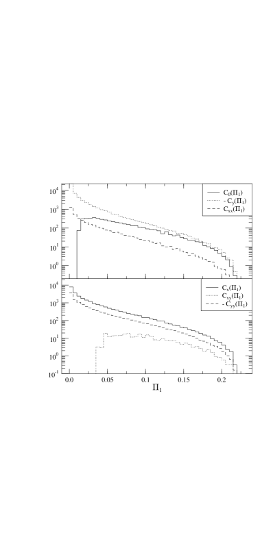
Figure 1: Next-to-leading order corrections to the group independent kinematical functions of the event shape variable $\Pi_{1}$.

We take SU(3) as underlying gauge group, and obtain the next-to-leading order prediction for the moments using the QCD values $x=9/4$ and $y=3/8$. The results — obtained for five light quark flavors at the $Z^{0}$ peak with $M_{Z}=91.187$ GeV, $\Gamma_{Z}=2.49$ GeV, $\sin^{2}\theta_{W}=0.23$ and ${\alpha_{s}}(M_{Z})=0.118$ — are plotted in Figure 2 and 3. The light grey bands indicate the renormalization scale dependence in the range $0.1<x_{\mu}=\mu/\sqrt{s}<2$ at leading order, while the dark bands show that at next-to-leading order. We see that the effect of the higher order correction is to increase the overall normalization, but no significant scale-dependence reduction occurs.

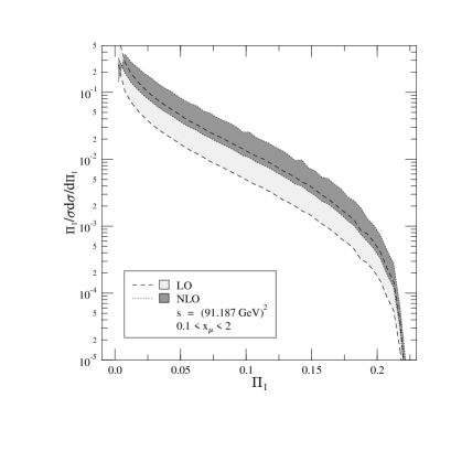
Figure 2: Next-to-leading order QCD prediction of the event shape variable $\Pi_{1}$.

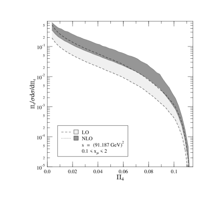
Figure 3: Next-to-leading order QCD prediction of the event shape variable $\Pi_{4}$.

In order to see the renormalization scale dependence in more details, we define the average value of these shape variables as

$$<O_{4}>=\frac{1}{\sigma}\int_{0}^{1}{\rm d}O_{4}\,O_{4}\frac{{\rm d}\sigma}{{\rm d}O_{4}}\>,$$ (9)

and study the dependence of the average value of the $\Pi_{1}$ variable on the scale in Figure 4. We see that there remains substantial scale dependence at next-to-leading order showing that the uncalculated higher order corrections are presumably large. The feature is similar for the $\Pi_{4}$ variable, but the residual scale dependence is even larger.

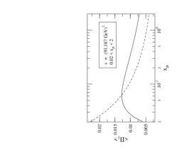
Figure 4: Renormalization scale dependence of the average value of the moment $\Pi_{1}$.

The same conclusion is drawn if we look at the dependence of the K factors on the observables as depicted in Figure 5. In case of the $\Pi_{1}$ parameter the K factor is slightly above two for the whole range, while for $\Pi_{4}$ it is even larger. This suggests that $\Pi_{4}$ cannot be reliable calculated in perturbation theory.

Figure 5: K factors of the $\Pi_{1}$ and $\Pi_{4}$ moments.

5 CONCLUSION

In this talk we presented for the first time a next-to-leading order calculation of the differential cross section of two four jet shape variables, the $\Pi_{1}$ and $\Pi_{4}$ Fox-Wolfram moments. We gave explicit results both for the full next-to-leading order cross sections and for the group independent kinematical functions of the radiative corrections. The effect of the radiative correction was to increase the overall normalization, but not to reduce the renormalization scale dependence significantly.

These results were produced by a partonic Monte Carlo program DEBRECEN that can be used for the calculation of QCD radiative corrections to the differential cross section of any kind of infrared safe four-jet observable in electron-positron annihilation.

We thank L. Dixon for providing us the Mathematica files of the one-loop four-parton helicity amplitudes.

6 DISCUSSIONS

A.P. Contogouris, Universtity of Athens
To produce your K factors you need a jet algorithm; however, there are more than one algorithms. Do I understand correctly that your K factors much depend on it?

Z. Trócsányi
The K factors do depend on the observable. This is also the case for three-jet observables. The smaller K factor the more reliable the quantity can be calculated in perturbation theory. From this point of view the Durham jet clustering algorithm (K$\simeq$1.6) is a better observable than the event shape variables.

A.P. Contogouris
Suppose you compare some of your K factors with those for three-jet production in $e^{+}e^{-}$ annihilation, corresponding to equivalent observables (e.g. shape variable). How do your K factors compare? Also, how do they compare with Drell-Yan lepton pari production, one of the first processes for which K-factors were calculated?

Z. Trócsányi
The K factor for the C parameter for instance, is about 1.5, i.e. much smaller than in our case. The Drell-Yan K factor is 1.8–2, which is again quite large, but somwhat smaller than our values.

References

- [1] B. Adeva et al, L3 Collaboration, Phys. Lett. B248 (1997) 227; P. Abreu et al, DELPHI Collaboration, Zeit. Phys. C 59 (1993) 357; R. Akers et al, OPAL Collaboration, Zeit. Phys. C 65 (1995) 367; R. Barate et al, ALEPH Collaboration, preprint CERN-PPE/97-002.
- [2] G.C. Fox and S. Wolfram, Phys. Lett. 82B (1979) 134.
- [3] W.T. Giele and E.W.N. Glover, Phys. Rev. D 46 (1992) 1980; W.T. Giele, E.W.N. Glover and D.A. Kosower, Nucl. Phys. B403 (1993) 633.
- [4] S. Frixione, Z. Kunszt and A. Signer, Nucl. Phys. B467 (1996) 399; Z. Nagy and Z. Trócsányi, Nucl. Phys. B486 (1997) 189; S. Frixione, preprint hep-ph/9706545.
- [5] S. Catani and M.H. Seymour, Phys. Lett. B378 (1996) 287, Nucl. Phys. 485 (1997) 291.
- [6] K. Hagiwara and D. Zeppenfeld, Nucl. Phys. B313 (1989) 560; F.A. Berends, W.T. Giele and H. Kuijf, Nucl. Phys. B321 (1989) 39; N.K. Falk, D. Graudenz and G. Kramer, Nucl. Phys. B328 (1989) 317.
- [7] E.W.N. Glover and D.J. Miller, Phys. Lett. B396 (1997) 257; J.M. Campbell, E.W.N. Glover and D.J. Miller, preprint hep-ph/9706297.
- [8] Z. Bern, L. Dixon and D. A. Kosower, Ann. Rev. Nucl. Part. Sci. 46 (1996) 109.
- [9] Z. Bern, L. Dixon, D. A. Kosower and S. Wienzierl, Nucl. Phys. B489 (1997) 3.
- [10] Z. Bern, L. Dixon and D. A. Kosower, preprint hep-ph/9708239.
- [11] Z. Nagy and Z. Trócsányi, preprint hep-ph/9708342.
- [12] A. Signer and L. Dixon, Phys. Rev. Lett. 78 (1997) 811; L. Dixon and A. Signer, preprint hep-ph/9706285.
- [13] S. Catani, Yu.L. Dokshitzer, M. Olsson, G. Turnock and B.R. Webber, Phys. Lett. B269 (1991) 432.
- [14] S. Bethke, Z. Kunszt, D.E. Soper and W.J. Stirling, Nucl. Phys. B370 (1992) 310.
- [15] N. Brown and W.J. Stirling, Zeit. Phys. C 53 (1992) 629.
- [16] Z. Nagy and Z. Trócsányi, preprint hep-ph/9707309.