Excluding light gluinos using four-jet LEP events: a next-to-leading order result

Abstract

Based upon a next-to-leading order perturbative calculation of the four-jet production rate in electron-positron annihilation and assuming 8 % for the theoretical error emerging from hadronization effects in the $0.002\leq y_{\rm cut}\leq 0.004$ range for the Durham clustering algorithm, we exclude the existence of the light gluinos at the 95 % confidence level.

In recent years several interesting phenomena were observed that could be naturally explained by the existence of light (with mass of the order of few GeV) supersymmetric partner of the gluon — the gluino [1, 2]. If light gluino exists, it should be produced at LEP. Gluinos do not couple directly to quarks, but a gluon can decay into a gluino pair. Thus the numerical value of four-jet observables should be different if gluinos exist than predicted by pure Quantum Chromodynamics (QCD). In particular, the measurement of the eigenvalues of the Casimir operators of the underlying Lie group, the color charges is based upon measuring four-jet observables, and this should also be influenced by the existence of light gluinos. This fact have been utilized by all LEP experiments for setting exclusion limits for the existence of light gluinos [3, 4, 5]. However, these analyses were based upon leading order calculation of the four-jet observables and as a consequence the exclusion limits are debated [4, 5, 6, 7].

Recently Dixon and Signer [8] and also ourselves [9] have completed the calculation of four-jet cross sections in electron-positron annihilation at the next-to-leading order accuracy. In this letter we extend the second of these works to including the effect of light gluinos. We present the cross sections in terms of group independent kinematical functions multiplying the eigenvalues of the Casimir operators of the underlying Lie group. The knowledge of the O($\alpha_{s}^{3}$) corrections to the group independent kinematical functions facilitates the simultaneous precision meaurement of the strong coupling and the color charge factors using the four-jet LEP or SLC data assuming any number of light gluino flavors. Thus in a full analysis the fit of the theoretical prediction to the data can reveal the number of light gluino flavors favoured by data. In this letter we do not perform such a full analysis. Instead, we point out that in the small $y_{\rm cut}$ region ($y_{\rm cut}\leq 0.004$) already the four-jet rate predicted for the light-gluino scenario significantly differs from the recent ALEPH data [10], while the QCD prediction is in good agreement with the experimental results.

The main ingredients of the calculation are the four-parton next-to-leading order and five-parton Born level squared matrix elements. The tree level amplitudes for the processes $e^{+}e^{-}\to{\bar{q}}qggg$ and $e^{+}e^{-}\to{\bar{q}}q{\bar{Q}}Qg$ have been known for a long time [11]. The new techniques developed by Bern, Dixon and Kosower in the calculation of one-loop multiparton amplitudes [12] made possible the derivation of explicit analytic expressions for the helicity amplitudes of the $e^{+}e^{-}\to Z^{0},\,\gamma^{*}\to$ 4 partons processes [13]. Also, Campbell, Glover and Miller made FORTRAN programs for calculating higher order corrections to the $e^{+}e^{-}\to\gamma^{*}\to$ 4 partons processes publicly available [14]. In all of these calculations, and also in our work, the quark and lepton masses are set to zero.

We use the matrix elements of refs. [13] for the loop corrections of the QCD subprocesses. As pointed out in refs. [6, 8], the naive ${N_{\rm f}}=5\to{N_{\rm f}}=8$ shift for taking into account the effect of the light gluinos is not valid exactly at the next-to-leading order accuracy. Analyzing the color structure of the diagrams involving gluinos and using the results of refs. [13] we have derived the necessary loop corrections for the process $e^{+}e^{-}\to Z^{0},\,\gamma^{*}\to{\bar{q}}q{\tilde{g}}{\tilde{g}}$ and the modifications induced by the presence of the gluinos on the four-parton one-loop QCD amplitudes [15]. We have also derived the $e^{+}e^{-}\to{\bar{q}}q{\tilde{g}}{\tilde{g}}g$ tree-level amplitudes.

It is well known that the next-to-leading order correction is a sum of two integrals — the real and virtual corrections — that are separately divergent (in the infrared) in $d=4$ dimensions. For infrared safe observables, for instance the four-jet rates used in this work, their sum is finite. In order to obtain this finite correction, we use a slightly modified version of the dipole method of Catani and Seymour [16] that exposes the cancellation of the infrared singularities directly at the integrand level. The formal result of this cancellation is that the next-to-leading order correction is a sum of two finite integrals,

$$\sigma^{\rm NLO}=\int_{5}{\rm d}\sigma_{5}^{\rm NLO}+\int_{4}{\rm d}\sigma_{4}^{\rm NLO}\>,$$ (1)

where the first term is an integral over the available five-parton phase space (as defined by the jet observable) and the second one is an integral over the four-parton phase space.

Once the phase space integrations in eq. (1) are carried out, the next-to-leading order differential cross section for the four-jet observable $O_{4}$ takes the general form

$$\frac{1}{\sigma_{0}}\frac{{\rm d}\sigma}{{\rm d}O_{4}}(O_{4})=\left(\frac{{\alpha_{s}}(\mu)C_{F}}{2\pi}\right)^{2}{\cal B}_{O_{4}}(O_{4})$$ (2)

$$\qquad+\left(\frac{{\alpha_{s}}(\mu)C_{F}}{2\pi}\right)^{3}\left[{\cal B}_{O_{4}}(O_{4})\frac{\beta_{0}}{C_{F}}\ln\frac{\mu^{2}}{s}+{\cal C}_{O_{4}}(O_{4})\right]\>.$$ (3)

In this equation $\sigma_{0}$ denotes the Born cross section for the process $e^{+}e^{-}\to{\bar{q}}q$, $s$ is the total c.m. energy squared, $\mu$ is the renormalization scale, while ${\cal B}_{O_{4}}$ and ${\cal C}_{O_{4}}$ are scale independent functions, ${\cal B}_{O_{4}}$ is the Born approximation and ${\cal C}_{O_{4}}$ is the radiative correction. We use the two-loop expression for the running coupling,

$${\alpha_{s}}(\mu)=\frac{{\alpha_{s}}(M_{Z})}{w(\mu)}\left(1-\frac{\beta_{1}}{\beta_{0}}\frac{{\alpha_{s}}(M_{Z})}{2\pi}\frac{\ln(w(\mu))}{w(\mu)}\right)\>,$$ (4)

with

$$w(\mu)=1-\beta_{0}\frac{{\alpha_{s}}(M_{Z})}{2\pi}\ln\left(\frac{M_{Z}}{\mu}\right)\>,$$ (5)

$$\beta_{0}=\frac{11}{3}C_{A}-\frac{4}{3}\left(T_{R}{N_{\rm f}}+\frac{1}{2}C_{A}{N_{\rm lg}}\right)\>,$$ (6)

$$\beta_{1}=\frac{17}{3}C_{A}^{2}-2C_{F}T_{R}{N_{\rm f}}-\frac{10}{3}C_{A}T_{R}{N_{\rm f}}-\frac{8}{3}C_{A}^{2}{N_{\rm lg}}\>,$$ (7)

for ${N_{\rm lg}}$ number of light gluino flavors [17], and with the normalization $T_{R}=1/2$ in ${\rm Tr}(T^{a}T^{{\dagger}b})=T_{R}\delta^{ab}$. The numerical values presented in this letter were obtained at the $Z^{0}$ peak with $M_{Z}=91.187$ GeV, $\Gamma_{Z}=2.49$ GeV, $\sin_{W}^{2}\theta=0.23$, ${\alpha_{s}}(M_{Z})=0.118$ and ${N_{\rm f}}=5$ light quark flavors.

In the case of jet rates it is customary to normalize the cross section to the O$({\alpha_{s}})$ total cross section, $\sigma_{\rm tot}=\sigma_{0}\left(1+{\alpha_{s}}/\pi\right)$. Then the four-jet rate can be written as

$$R_{4}(y_{\rm cut})=\frac{1}{\sigma_{\rm tot}}\int_{\infty}^{y_{\rm cut}}{\rm d}y\frac{{\rm d}\sigma_{4}}{{\rm d}y}(y)$$ (8)

$$=\left(1+\frac{{\alpha_{s}}}{\pi}\right)^{-1}\left(\frac{{\alpha_{s}}C_{F}}{2\pi}\right)^{2}$$ (9)

$$\left\{B_{4}(y_{\rm cut})+\left(\frac{{\alpha_{s}}C_{F}}{2\pi}\right)\left[B_{4}(y_{\rm cut})\frac{\beta_{0}}{C_{F}}\ln\frac{\mu^{2}}{s}+C_{4}(y_{\rm cut})\right]\right\}\>,$$ (10)

where the scale dependence in ${\alpha_{s}}$ has been suppressed. The Born approximation and the higher order correction are linear and quadratic forms of ratios of the color charges [15]:

$$B_{4}=B_{0}+B_{x}\,x+B_{y}\,y\>,$$ (11)

and

$$C_{4}=C_{0}+\,C_{x}\,x+C_{y}\,y+C_{z}\,z$$ (12)

$$\quad\;\;+\,C_{xx}\,x^{2}+C_{xy}\,x\,y+C_{yy}\,y^{2}\>.$$ (13)

The $x$ and $y$ parameters are ratios of the quadratic Casimirs, $x=C_{A}/C_{F}$ and $y=T_{R}/C_{F}$, while $z$ is related to the square of a cubic Casimir,

$$C_{3}=\sum_{a,b,c=1}^{N_{A}}{\rm Tr}(T^{a}T^{b}T^{{\dagger}c}){\rm Tr}(T^{{\dagger}c}T^{b}T^{a})\>,$$ (14)

via $z=\frac{C_{3}}{{N_{C}}C_{F}^{3}}$. We plot the numerical values for the correction functions $C_{i}$ for the case of Durham clustering algorithm [18] in Fig. 1. Note that the $C_{z}$ function is completely negligible, therefore it is not plotted. In order to exhibit the behaviour in the small $y_{\rm cut}$ region, the correction functions are plotted against $L^{4}$, where $L=\ln(1/y_{\rm cut})$.

Using these group independent kinematical functions one can fit the observed data for the best values of the color factor ratios $x$ and $y$ in both theories separately, and test how the obtained results are compatible with the SU(3) values $x=9/4$ and $y=3/8$. In principle, any kind of four-jet observable can be used for this purpose. In practice, various normalized angular distributions were used [19]. These observables have the virtue that their renormalization scale dependence is very small already at tree level due to the normalization, therefore they can be calculated reliably at leading order. Indeed, this has been shown to be the case in the next-to-leading order calculation in ref. [20] and we confirm that result. We should like to emphasize however, that the small scale dependence of the tree-level perturbative result does not necessary mean that the results for the exclusion of light gluinos from color charge measurement are insensitive to the higher order corrections. Fig. 1 shows that the $C_{x}$, $C_{xx}$ and $C_{xy}$ kinematical functions change substantially, while the $C_{y}$ and $C_{yy}$ functions remain unchanged with the inclusion of the additional degrees of freedom. This may modify the result of the fit for the color charges.

We do not perform the complete color charge analysis here, but note that this approach is slightly different from the effective number of flavors approach, where the same best fit for both theories is made and this unique result is compared with $x=9/4$ and $y_{\rm eff}=3/5$ with the effective $y_{\rm eff}$ value obtained from the ${N_{\rm f}}=5\to 8$ rule. This latter method is made possible by the simplicity of the tree-level matrix elements, but strictly speaking is not valid in a next-to-leading order analysis.

In this letter we simply take values in SU(3) for the color factor ratios and using our kinematical functions we predict the numerical values for the Born and correction functions $B_{4}(y_{\rm cut})$ and $C_{4}(y_{\rm cut})$ in both theories. These functions are then fitted according to the formula [22]

$$F(y_{\rm cut})=\sum_{n=0}^{N_{F}}k_{n}L^{n}\>,$$ (15)

where $F=B_{4}$, or $C_{4}$. The coefficients $k_{n}$ are tabulated in Table I. The fit-range is 0.002–0.1. The QCD results agree with the rates obtained by Dixon and Signer [8].

Using the $B_{4}$ and $C_{4}$ functions, we construct $R_{4}(y_{\rm cut})$ according to formula (8). We see that for small values of resolution parameter, $y_{\rm cut}\leq 0.004$, the predictions for the QCD and QCD + light gluino case start to differ. For small values of $y_{\rm cut}$ however, the fixed order perturbative prediction is not reliable, because the expansion parameter ${\alpha_{s}}\ln^{2}y_{\rm cut}$ logarithmically enhances the higher order corrections. The usual remedy is the all order resummation of the leading and next-to-leading logarithmic contributions and matching the resummed and fixed order results [21]. We use R-matching as described in refs. [21, 8].

Fig. 2 shows the effect of resummation and matching in QCD (${N_{\rm lg}}=0$). We see that the resummed and matched prediction agrees with the ALEPH data corrected to hadron level [10] within hadronization uncertainty. Encouraged by this, in the same figure we plot the fixed order and the resummed and matched SU(3) predictions for the QCD + light gluino scenario (${N_{\rm lg}}=1$). The bands indicate the theoretical uncertainty of the fixed order prediction due to the variation of the renormalization scale $x_{\mu}=\mu/\sqrt{s}$ between 1/2 and 2. The data are well described by the QCD prediction in the whole $y_{\rm cut}$ range, but they fall outside the QCD + light gluino band. For values of $y_{\rm cut}\leq 0.004$ the theoretical bands bifurcate making the discrepancy between the two theories significant.

In order to quantify the exclusion level of the very light gluino, we plot the scale dependence of the next-to-leading order prediction at a fix value of $y_{\rm cut}=0.002$ in Fig. 3. Our choice for this value of the resolution parameter comes from the observation that in Fig. 2 the intercept of the ${N_{\rm lg}}=0$ theoretical curves for the O$({\alpha_{s}}^{3})$ and O$({\alpha_{s}}^{3})$+NLLA prediction at $x_{\mu}=1$ is around 0.002, showing that in this region the fixed order prediction itself can be trusted. Also around $y_{\rm cut}=0.002$ the hadronization effects are still small [23, 24].

From Fig. 3 we see that the QCD prediction agrees well with the measured data, while the QCD + light gluino prediction falls significantly below. Taking the renormalization scale dependence as the theoretical error, the light gluino is excluded at more than $4\sigma$, or 99.99 % confidence level. The theoretical prediction for the two theories differ at the $\simeq 85$ % confidence level. The $y_{\rm cut}=0.002$ value at LEP corresponds to a $k_{\perp}\simeq 5\,$GeV, where the theoretical error emerging form hadronization does not exceed 8 % [23]. Therefore, with hadronization uncertainty included the QCD + light gluino prediction is still excluded at the $2\sigma$, or 95 % confidence level. According to Fig. 2, the effect of resummation of leading and next-to-leading $\ln(1/y_{\rm cut})$ logarithms is to make the exclusion even more significant.

Finally, we would like to remark that the inclusion of the non-zero gluino mass decreases the tree-level cross section [2]. The K factor for the QCD + light gluino theory is small, $K\simeq 1.25$, suggesting that this mass effect is bound to be robust when including the higher orders.

In this letter we presented the next-to-leading order corrections to the gauge independent kinamatical functions of the four-jet rate cross section in QCD and in QCD with the extension of light gluinos for the case of the Durham clustering algorithm. The knowledge of these corrections facilitates the simultaneous precision meaurement of the strong coupling and the color charge factors using the four-jet LEP or SLC data assuming any number of light gluino flavors. Assuming standard SU(3) values for the color factors, we presented the four-jet rates as predicted by next-to-leading order perturbation theory matched with all order resummed results in the next-to-leading logarithmic approximation. These theoretical predictions were compared to recent data obtained by the ALEPH collaboration. The four-jet rates in the QCD and QCD + light gluino scenario are significantly different for small values of the resolution parameter $y_{\rm cut}$. The data favour the gluinoless world, excluding the existence of light gluinos at the 95 % level. This result was argued to be robust against hadronization and gluino mass effects. Our results also show that a conventional color charge measurement based on angle distributions should give the most significant light gluino exclusion limit if the jets are defined at small $y_{\rm cut}$, ($y_{\rm cut}<0.004$).

We thank L. Dixon for providing Mathematica files of the one-loop helicity amplitudes, furthermore S. Catani and G. Dissertori for helpful correspondence. This research was supported in part by the EEC Programme ”Human Capital and Mobility”, Network ”Physics at High Energy Colliders”, contract PECO ERBCIPDCT 94 0613 as well as by the Hungarian Scientific Research Fund grant OTKA T-016613.

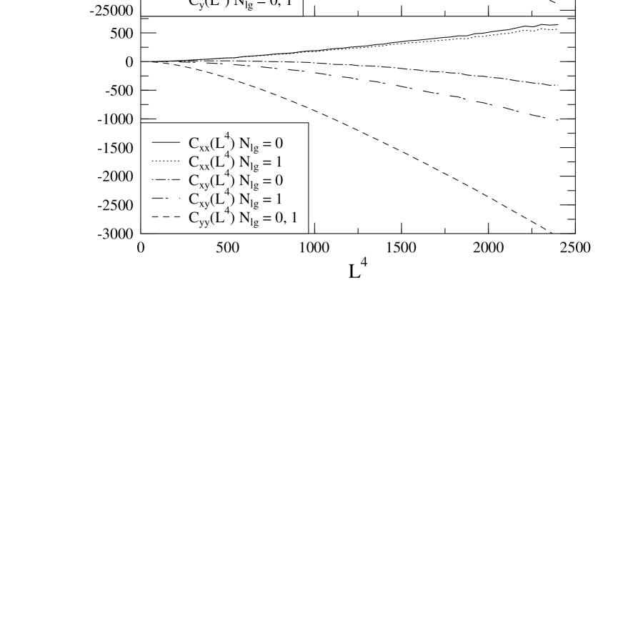
FIG. 1.: Group independent kinematical functions $C_{i}$ for QCD and QCD + light gluino theory.

TABLE I.: Coefficients of the analytic fits for the Born level and next-to-leading order scale independent functions $B_{4}$ and $C_{4}$. First two rows for QCD, second two rows for QCD + light gluino theory.

F	$k_{0}$	$k_{1}$	$k_{2}$	$k_{3}$	$k_{4}$	$k_{5}$	$k_{6}$
$B_{4}$	-0.744	-8.224	13.034	-6.5152	1.0736
$C_{4}$	1363	-2742	2102	-720.4	85.2	5.68	-1.0712
$B_{4}$	-1.758	-7.02	12.663	-6.545	1.0941
$C_{4}$	528.1	-1158.53	891.56	-250.47	-10.945	15.821	-1.64

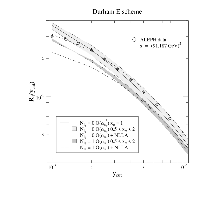
FIG. 2.: Full next-to-leading order and resummed-matched four-jet rate in QCD + ${N_{\rm lg}}=0,1$ compared to ALEPH data.

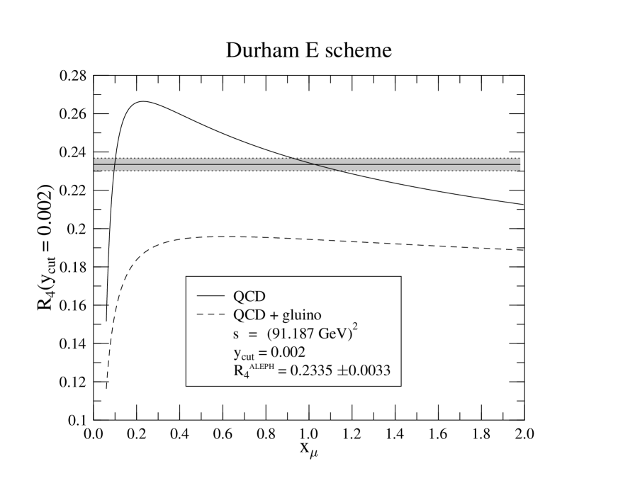
FIG. 3.: Renormalization scale dependence of the next-toleading order prediction for the four-jet rate at $y_{\rm cut}=0.002$. The grey band indicates the value measured by ALEPH, corrected to hadron level.

REFERENCES

- [1] G.R. Farrar, Phys. Lett. B265, 395 (1991); Phys. Rev. D 51, 3904 (1995);F.E. Close, G.R. Farrar and Z.P. Li, Phys. Rev. D 55, 5749 (1997);G.R. Farrar, preprint hep-ph/9704309; D.J. Chung, G.R. Farrar and E.W. Kolb, preprint astro-ph/9707036; J. Ellis, D. Nanopoulos and D. Ross, Phys. Lett. B305, 375 (1993).
- [2] R. Muoz-Tapia and W.J. Stirling, Phys. Rev. D 49, 3763 (1994).
- [3] B. Adeva et al, L3 Collaboration, Phys. Lett. B248, 227 (1990). P. Abreu et al, DELPHI Collaboration, Zeit. Phys. C 59, 357 (1993).
- [4] R. Akers et al, OPAL Collaboration, Zeit. Phys. C 65, 367 (1995).
- [5] R. Barate et al, ALEPH Collaboration, preprint CERN-PPE/97-002.
- [6] F. Csikor and Z. Fodor, Phys. Lett. 78, 4335 (1997).
- [7] A. de Gouvea and H. Murayama, Phys. Lett. B400, 117 (1997); G.R. Farrar, hep-ph/9707467.
- [8] L. Dixon and A. Signer, Phys. Rev. Lett. 78, 811 (1997); preprint hep-ph/9706285.
- [9] Z. Nagy and Z. Trócsányi, preprint hep-ph/9707309.
- [10] R. Barate et al, ALEPH collaboration, preprint CERN-PPE-96-186.
- [11] K. Hagiwara and D. Zeppenfeld, Nucl. Phys. B313, 560 (1989); F.A. Berends, W.T. Giele and H. Kuijf, Nucl. Phys. B321, 39 (1989); N.K. Falk, D. Graudenz and G. Kramer, Nucl. Phys. B328, 317 (1989).
- [12] Z. Bern, L. Dixon and D. A. Kosower, Ann. Rev. Nucl. Part. Sci. 46 (1996) 109.
- [13] Z. Bern, L. Dixon, D. A. Kosower and S. Wienzierl, Nucl. Phys. B489, 3 (1997); Z. Bern, L. Dixon and D. A. Kosower, preprint hep-ph/9708239.
- [14] E.W.N. Glover and D.J. Miller, Phys. Lett. B396, 257 (1997); J.M. Campbell, E.W.N. Glover and D.J. Miller, preprint hep-ph/9706297.
- [15] Z. Nagy and Z. Trócsányi, preprint hep-ph/9708342.
- [16] S. Catani and M.H. Seymour, Phys. Lett. B378, 287 (1996), Nucl. Phys. 485, 291 (1997).
- [17] S. Dimopoulos, S.Raby and F. Wilczek, Phys. Rev. D 24, 1681 (1981); L.E.Ibanez and G.G. Ross, Phys. Lett. B105, 439 (1981); W.J. Marciano and G.Senjanovic, Phys. Rev. D 25, 3092 (1982); M.B. Einhorn and D.R.T. Jones, Nucl. Phys. B196, 475 (1982).
- [18] S. Catani et al, Phys. Lett. B269, 432 (1991).
- [19] J.G. Körner, G. Schierholz and J. Willrodt, Nucl. Phys. B185, 365 (1981); O. Nachtman and A. Reiter, Zeit. Phys. C 16, 45 (1982); M. Bengtsson and P.M. Zerwas, Phys. Lett. B208, 306 (1988).
- [20] A. Signer, preprint hep-ph/9705218.
- [21] Catani et al, Phys. Lett. B269, 432 (1991).
- [22] S. Bethke et al, Nucl. Phys. B370, 310 (1992).
- [23] B.R. Webber, in Proceedings of the International Conference ‘QCD — 20 years later’, ed.: P.M. Zerwas and H.A. Kastrup, World Scientific (1993).
- [24] S. Catani et al, Nucl. Phys. B377, 445 (1992).