Abstract
Padé approximants are used to improve the convergence behavior of perturbative results in massless scalar and gauge field theories at finite temperature.

In recent years, computational methods have been developed to analytically tackle three-loop vacuum diagrams and higher-order contributions of diagrams with less loops in massless field theories at finite temperature [1]-[5]. Consequently, the free energy density $F$ at zero chemical potential could be computed analytically at the $g^{5}$ level in both massless $g^{2}\phi^{4}$ theory [3] (the pressure given there is the negative of the free energy density) and in massless gauge theories [5, 6]. In [5]-[7], specializations to QED can be found, where the result was known before in partially numerical form [2].

However, for interesting values of the coupling constant in non-Abelian gauge theories, the convergence behavior of the perturbative series is not convincing [5, 6]. In this brief report, we note that the use of Padé approximants drastically improves this behavior in both $\phi^{4}$ and gauge theories. For the use of Padé approximants and other resummation techniques in other contexts in perturbative field theory and statistical physics, see, e.g., [8], and references therein.

Let us first review those features of the results of [3, 5, 6] which are essential for our analysis here. The perturbative series for the free energy density in both scalar and gauge theories has the structure (see the appendix for details)

$$F=T^{4}[c_{0}+c_{2}g^{2}+c_{3}g^{3}+(c_{4a}\ln g+c_{4b})g^{4}+(c_{5a}\ln g+c_{5b})g^{5}+O(g^{6}\ln g)]\,,$$ (1)

where $T$ is the temperature and $c_{0}$, $c_{2}$, $c_{3}$, $c_{4a}$, $c_{5a}$ are constants, while $c_{4b}$ and $c_{5b}$ have a logarithmic dependence on $\ln(\bar{\mu}/T)$, where $\bar{\mu}$ is the renormalization scale in the modified minimal subtraction scheme ($\overline{\mbox{MS}}$). In $\phi^{4}$ theory, $c_{4a}=0$, while in gauge theories $c_{5a}=0$.

As in [5], we use the renormalization group to make $g^{2}$ running,

$$\frac{1}{g^{2}(\bar{\mu})}\approx\frac{1}{g_{T}^{2}}-\beta_{0}\ln\frac{\bar{\mu}}{T}+\frac{\beta_{1}}{\beta_{0}}\ln\left(1-\beta_{0}g_{T}^{2}\ln\frac{\bar{\mu}}{T}\right)\,,$$ (2)

where $\beta_{0}$ and $\beta_{1}$ are the one- and two-loop coefficients of the beta function $\beta_{g}$ of $g^{2}$ (see the appendix for details on $\beta_{0}$ and $\beta_{1}$), and $g_{T}$ is the coupling constant at temperature $T$. Then $g$ in (1) is replaced by $g(\bar{\mu})$. In this way we get an idea of the dependence of our result on the choice of renormalization scale. We could subsequently expand $F$ in powers of $g_{T}$ to check that $F$ becomes explicitly independent of $\bar{\mu}$ through $g_{T}^{5}$. For this purpose, we would really only need the one-loop coefficient of $\beta_{g}$. The reason is that $\beta_{g}$ contains only even powers of $g$, $\beta_{g}=\beta_{0}g^{4}+\beta_{1}g^{6}+\cdots$, since we renormalize as at zero temperature. Therefore, from the viewpoint of the renormalization group, the $g^{4}$ and $g^{5}$ terms in $F$ are the first corrections to the $g^{2}$ and $g^{3}$ terms, respectively. Numerically, the difference between using $\beta_{g}$ to one or two loops is insignificant for the examples in non-Abelian gauge theories below, but keeping the two-loop correction turns out to improve the behavior of the resummation in $\phi^{4}$ theory. The reason why it suffices to use the two-loop beta function in the examples in this work is that bad behavior of both the perturbative result and Pade approximants sets in for values of $g^{2}$ where the two-loop beta function is still a good approximation.

Now we use Padé approximants to reexpress $F$. For this purpose we pretend that $c_{4}\equiv c_{4a}\ln g+c_{4b}$ and $c_{5}\equiv c_{5a}\ln g+c_{5b}$ are constants in a Taylor series $F=T^{4}[c_{0}+c_{2}g^{2}+c_{3}g^{3}+c_{4}g^{4}+c_{5}g^{5}+\cdots]$. $c_{4}$ and $c_{5}$ have different values for each choice of $\bar{\mu}$ both through their direct dependence on $\ln(\bar{\mu}/T)$ and through the running of $g(\bar{\mu})$ in $\ln g$. Using the approximants [1/2], [2/2] and [2/3] to rewrite $F$ through orders $g^{3}$, $g^{4}$ and $g^{5}$ (there is no approximant [1/1], since $F$ contains no term linear in $g$) gives

$$F_{[1,2]} = \textstyle T^{4}\frac{c_{0}^{2}c_{2}-c_{0}^{2}c_{3}g}{c_{0}c_{2}-c_{0}c_{3}g-c_{2}^{2}g^{2}}\,,$$ (3)

$$F_{[2,2]} = \textstyle T^{4}\frac{c_{0}c_{2}^{2}-c_{0}c_{2}c_{3}g+(c_{2}^{3}+c_{0}c_{3}^{2}-c_{0}c_{2}c_{4})g^{2}}{c_{2}^{2}-c_{2}c_{3}g+(c_{3}^{2}-c_{2}c_{4})g^{2}}\,,$$ (4)

$$F_{[2,3]} = \textstyle T^{4}\frac{c_{0}(c_{2}^{3}+c_{0}c_{3}^{2}-c_{0}c_{2}c_{4})+c_{0}(-c_{2}^{2}c_{3}-c_{0}c_{3}c_{4}+c_{0}c_{2}c_{5})g+(c_{2}^{4}+2c_{0}c_{2}c_{3}^{2}-2c_{0}c_{2}^{2}c_{4}+c_{0}^{2}c_{4}^{2}-c_{0}^{2}c_{3}c_{5})g^{2}}{(c_{2}^{3}+c_{0}c_{3}^{2}-c_{0}c_{2}c_{4})+(-c_{2}^{2}c_{3}-c_{0}c_{3}c_{4}+c_{0}c_{2}c_{5})g+(c_{2}c_{3}^{2}-c_{2}^{2}c_{4}+c_{0}c_{4}^{2}-c_{0}c_{3}c_{5})g^{2}+(-c_{3}^{3}+2c_{2}c_{3}c_{4}-c_{2}^{2}c_{5})g^{3}}\,.$$ (5)

Define

$$\alpha(T)=g_{T}^{2}/(4\pi)$$ (6)

and let us look at some specific examples. Our first case is the small-coupling QCD example from [5] with $d_{A}=8$, $C_{A}=3$, $n_{f}=6$, $d_{F}=18$, $S_{F}=3$, $S_{2F}=4$, and $\alpha(T)=0.001$. As argued in [5] and as can be seen in Fig. 1a, the perturbative series for $F$ through $g^{5}$ is well behaved in this case, with respect to both convergence for a given renormalization scale $\bar{\mu}$ and to the growing $\bar{\mu}$ independence of $F$ towards higher orders. The Padé approximants $F_{[1,2]}$ and $F_{[2,2]}$ are close to the $g^{3}$ and $g^{4}$ results within the expected accuracy (given by the magnitude of the $g^{4}$ and $g^{5}$ corrections, respectively). However, $F_{[2,3]}$ has a pole, as seen in Fig. 1b. This pole comes about through a zero of the denominator in (5), which, in turn, due to the smallness of $\alpha(T)$, is caused by a zero of the first term in the denominator of (5), $c_{2}^{3}+c_{0}c_{3}^{2}-c_{0}c_{2}c_{4}$. We know that the full result for $F$ is independent of $\bar{\mu}$ and that consequently this pole is an artifact of the resummation scheme. We therefore determine its position and residue, explicitly remove it and call the resulting function $\bar{F}_{[2,3]}$. The curve in Fig. 1b for $\bar{F}_{[2,3]}$ is virtually identical to the $g^{5}$ result in the perturbative series in Fig. 1a.

Now let us turn to cases where the pure perturbative series needs improvement. Fig. 2a represents the perturbative series for the pure SU(2) example from [5] with $d_{A}=3$, $C_{A}=2$, $n_{f}=d_{F}=S_{F}=S_{2F}=0$, and $\alpha(T)=0.03$, while Fig. 2b shows the Padé approximants. Again, we have removed the pole from $F_{[2,3]}$ to define $\bar{F}_{[2,3]}$ and show both functions. Clearly, the convergence behavior of the series $F_{[1,2]}$, $F_{[2,2]}$, $\bar{F}_{[2,3]}$ is drastically improved compared to the purely perturbative series, particularly around natural choices of $\bar{\mu}$, such as $\bar{\mu}=T$ or $\bar{\mu}=gT$, which up to $g^{5}$ order are the only mass scales in finite-temperature non-Abelian gauge theories. Note also the relative independence from the renormalization scale.

Now turn to the other QCD example in [5], namely, $\alpha(T)=0.1$ with the other parameters being the same as in our first case. The result is plotted in Fig. 3. Again, there is much improvement compared to the pure perturbative series around $\bar{\mu}=T\approx gT$, where higher approximants give subsequently smaller corrections to their predecessors.

As our final example in non-Abelian gauge theories, consider three-flavor QCD, i.e., $d_{A}=8$, $C_{A}=3$, $n_{f}=3$, $d_{F}=9$, $S_{F}=3/2$, $S_{2F}=2$ with $\alpha(2\pi T)=1/3$ [note that we have to replace $T\rightarrow 2\pi T$ in (2) and (6) accordingly]. Up to the fact that we neglect the strange-quark mass and that we have set all chemical potentials to zero, this is close to the case of the quark-gluon plasma to be produced at the BNL Relativistic Heavy-Ion Collider (RHIC). The result is plotted in Fig. 4. There seems to be no useful improvement over the perturbative series, although the range of manifestly bad behavior is shifted towards smaller values of $\bar{\mu}$.

In Fig. 5, we present an example in scalar theory, namely with $\alpha(T)=0.75$. Note how, at least for not too big $\bar{\mu}$, the Padé approximants fluctuate much less in subsequent orders than their purely perturbative counterparts. The fact that we can go to larger couplings in scalar theory than in non-Abelian gauge theory is easily explained. For example, for the case of no fermions, the effective expansion parameter in $F$ is seen to be $C_{A}\alpha(T)$. That is, a larger number of degrees of freedom leads to stronger corrections to the ideal gas result (unless we try to make fermionic and bosonic contributions cancel).

Let us make two final remarks. (i) The use of the approximants [2/1] and [3/2] instead of [1/2] and [2/3] gives results very similar to those presented here, while approximants $[m/n]$ with $|m-n|>1$ give typically less improvement. (ii) Starting at $g^{6}$ order, another physical scale $g^{2}T$ enters the calculation of $F$ in non-Abelian gauge theories [9]. Therefore, it would be interesting to see how inclusion of the $g^{6}$ term changes our results. Unfortunately, computation of this term is difficult and requires a combination of perturbative and nonperturbative techniques [6, 10].

Appendix

Here we give the results of [3] and [5, 6].

With the Euclidean Lagrange density

$${\cal L}=\frac{1}{2}(\partial_{\mu}\phi)^{2}+\frac{g^{2}}{4!}\phi^{4}\,,$$ (7)

the free energy density in the $\overline{\mbox{MS}}$ scheme is

$$F = -\frac{\pi^{2}T^{4}}{9}\Bigg{\{}\frac{1}{10}-\frac{1}{8}\left(\frac{g}{4\pi}\right)^{2}+\frac{1}{\sqrt{6}}\left(\frac{g}{4\pi}\right)^{3}$$ (8)

$$\hskip 40.0pt-\left(\frac{g}{4\pi}\right)^{4}\left[-\frac{3}{8}\ln\frac{\bar{\mu}}{4\pi T}+\frac{1}{4}\frac{\zeta^{\prime}(-3)}{\zeta(-3)}-\frac{1}{2}\frac{\zeta^{\prime}(-1)}{\zeta(-1)}-\frac{1}{8}\gamma_{E}+\frac{59}{120}\right]$$

$$\hskip 40.0pt+\left(\frac{g}{4\pi}\right)^{5}\sqrt{\frac{3}{2}}\left[-\frac{3}{2}\ln\frac{\bar{\mu}}{4\pi T}+\frac{\zeta^{\prime}(-1)}{\zeta(-1)}-\frac{1}{2}\gamma_{E}-\frac{5}{4}+2\ln\left(\frac{g}{4\pi}\sqrt{\frac{2}{3}}\right)\right]\Bigg{\}}+O(g^{6}\ln g)\,,\hskip 20.0pt$$

where we have translated the MS result of [3] into $\overline{\mbox{MS}}$ using $\mu^{2}=e^{\gamma_{E}}\bar{\mu}^{2}/(4\pi)$ and where $\zeta$ is Riemann’s zeta function and $\gamma_{E}$ is the Euler-Mascheroni constant. The one- and two-loop coefficients in $\beta_{g}$ are

$$\beta_{0}=\frac{3}{(4\pi)^{2}}\,,\hskip 30.0pt\beta_{1}=-\frac{17}{3(4\pi)^{4}}\,.$$ (9)

In gauge theory with fermions with a single, simple Lie group consider the Euclidean Lagrange density

$${\cal L}=\bar{\psi}\gamma_{\mu}\left(\partial_{\mu}-igA_{\mu}^{a}T^{a}\right)\psi+\frac{1}{4}\left(\partial_{\mu}A_{\nu}^{a}-\partial_{\nu}A_{\mu}^{a}+gf^{abc}A_{\mu}^{b}A_{\nu}^{c}\right)^{2}\,,$$ (10)

where the $T^{a}$ are the generators of the group in the fermion representation. Let $d_{A}$ and $C_{A}$ be the dimension and quadratic Casimir invariant of the adjoint representation, with

$$\delta^{aa}=d_{A}\,,\hskip 20.0ptf^{abc}f^{dbc}=C_{A}\delta^{ad}\,.$$ (11)

Let $d_{F}$ be the dimension of the total fermion representation (e.g., 18 for six-flavor QCD), and define $S_{F}$ and $S_{2F}$ in terms of the generators $T^{a}$ for the total fermion representation as

$$S_{F}=\frac{1}{d_{A}}{\rm tr}(T^{2})\,,\hskip 20.0ptS_{2F}=\frac{1}{d_{A}}{\rm tr}[(T^{2})^{2}]\,,$$ (12)

where $T^{2}=T^{a}T^{a}$. For SU($N$) with $n_{F}$ fermions in the fundamental representation, the standard normalization of the coupling gives

$$d_{A}=N^{2}-1\,,\hskip 10.0ptC_{A}=N\,,\hskip 10.0ptd_{F}=Nn_{F}\,,\hskip 10.0ptS_{F}=\frac{1}{2}n_{F}\,,\hskip 10.0ptS_{2F}=\frac{N^{2}-1}{4N}n_{F}\,.$$ (13)

The the free energy density is given by

$$F = d_{A}T^{4}\frac{\pi^{2}}{9}\Bigg{\{}-\frac{1}{5}\left(1+\frac{7d_{F}}{4d_{A}}\right)+\left(\frac{g}{4\pi}\right)^{2}\left(C_{A}+\textstyle\frac{5}{2}S_{F}\right)$$ (14)

$$\hskip 50.0pt-48\left(\frac{g}{4\pi}\right)^{3}\left(\frac{C_{A}+S_{F}}{3}\right)^{3/2}-48\left(\frac{g}{4\pi}\right)^{4}C_{A}(C_{A}+S_{F})\ln\left(\frac{g}{2\pi}\sqrt{\frac{C_{A}+S_{F}}{3}}\right)$$

$$\hskip 50.0pt+\left(\frac{g}{4\pi}\right)^{4}\Bigg{[}C_{A}^{2}\left(\frac{22}{3}\ln\frac{\bar{\mu}}{4\pi T}+\frac{38}{3}\frac{\zeta^{\prime}(-3)}{\zeta(-3)}-\frac{148}{3}\frac{\zeta^{\prime}(-1)}{\zeta(-1)}-4\gamma_{E}+\frac{64}{5}\right)$$

$$\hskip 100.0pt+C_{A}S_{F}\left(\frac{47}{3}\ln\frac{\bar{\mu}}{4\pi T}+\frac{1}{3}\frac{\zeta^{\prime}(-3)}{\zeta(-3)}-\frac{74}{3}\frac{\zeta^{\prime}(-1)}{\zeta(-1)}-8\gamma_{E}+\frac{1759}{60}+\frac{37}{5}\ln 2\right)$$

$$\hskip 100.0pt+S_{F}^{2}\left(-\frac{20}{3}\ln\frac{\bar{\mu}}{4\pi T}+\frac{8}{3}\frac{\zeta^{\prime}(-3)}{\zeta(-3)}-\frac{16}{3}\frac{\zeta^{\prime}(-1)}{\zeta(-1)}-4\gamma_{E}-\frac{1}{3}+\frac{88}{5}\ln 2\right)$$

$$\hskip 100.0pt+S_{2F}\left(-\frac{105}{4}+24\ln 2\right)\Bigg{]}$$

$$\hskip 50.0pt-\left(\frac{g}{4\pi}\right)^{5}\left(\frac{C_{A}+S_{F}}{3}\right)^{1/2}\Bigg{[}C_{A}^{2}\left(176\ln\frac{\bar{\mu}}{4\pi T}+176\gamma_{E}-24\pi^{2}-494+264\ln 2\right)$$

$$\hskip 175.0pt+C_{A}S_{F}\left(112\ln\frac{\bar{\mu}}{4\pi T}+112\gamma_{E}+72-128\ln 2\right)$$

$$\hskip 175.0pt+S_{F}^{2}\left(-64\ln\frac{\bar{\mu}}{4\pi T}-64\gamma_{E}+32-128\ln 2\right)$$

$$\hskip 175.0pt-144S_{2F}\Bigg{]}+O(g^{6})\Bigg{\}}\,.$$

The one- and two-loop coefficients in $\beta_{g}$ are

$$\beta_{0}=\frac{1}{(4\pi)^{2}}\left(-\frac{22}{3}C_{A}+\frac{8}{3}S_{F}\right)\,,\hskip 30.0pt\beta_{1}=\frac{1}{(4\pi)^{4}}\left(-\frac{68}{3}C_{A}^{2}+\frac{40}{3}C_{A}S_{F}+8S_{2F}\right)\,.$$ (15)

Fig. 1a

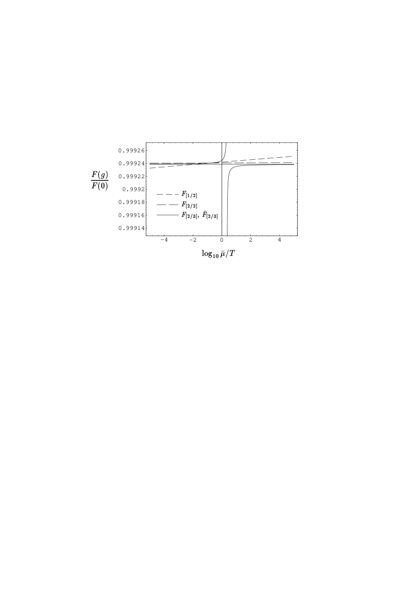
Fig. 1b

Figure 1: Fig. 1a shows the perturbative series for the free energy density in units of the ideal gas result $F(g=0)$ for six-flavor QCD with $\alpha(T)=0.001$ for a range of choices of renormalization scale $\bar{\mu}$. The short-dashed, medium-dashed, long-dashed and solid lines are the results for $F$ including terms through orders $g^{2}$, $g^{3}$, $g^{4}$ and $g^{5}$, respectively. Fig. 1b shows Padé approximants instead: The $g^{2}$ result has been dropped, while the result through $g^{3}$ from Fig. 1a has been replaced by $F_{[1/2]}$, the result through $g^{4}$ by $F_{[2/2]}$ and the result through $g^{5}$ by $F_{[2/3]}$ (solid line with pole) and $\bar{F}_{[2/3]}$ (solid line without pole).

Fig. 2a

Fig. 2b

Figure 2: The same as Fig. 1, but for pure SU(2) theory with $\alpha(T)=0.03$.

Fig. 3a

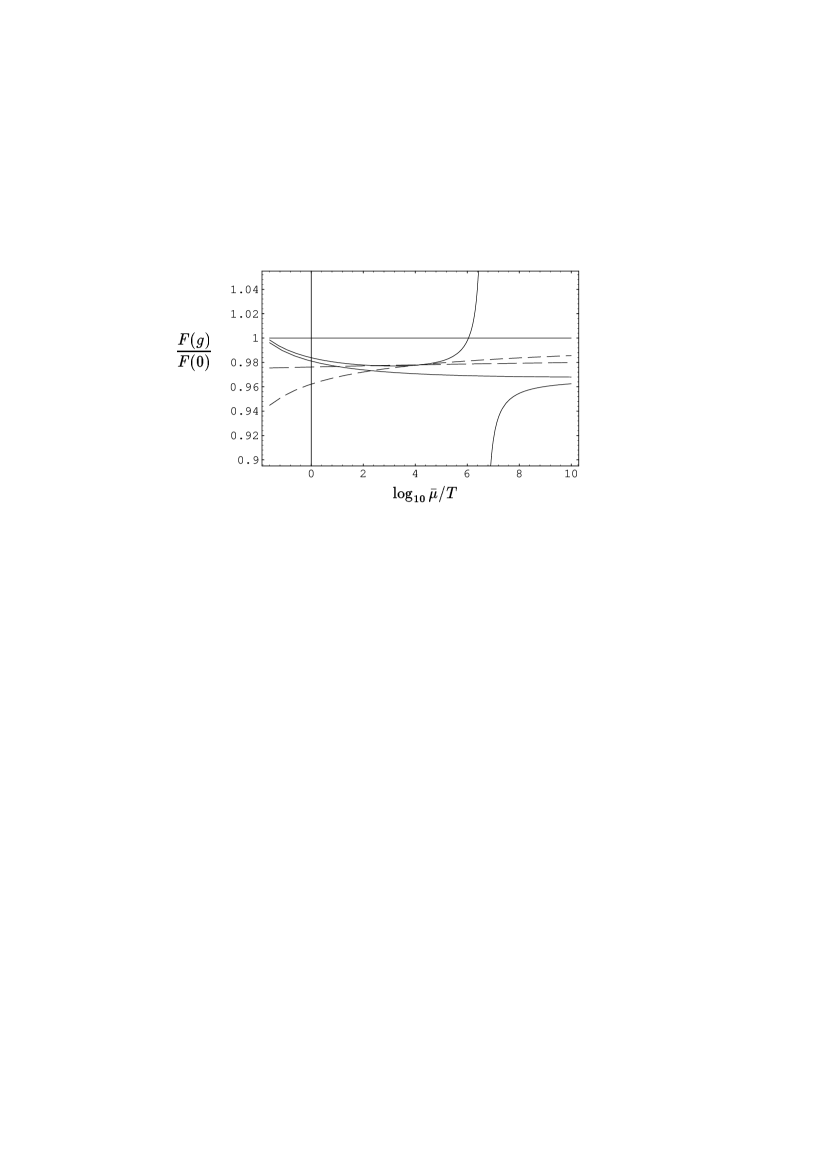
Fig. 3b

Figure 3: The same as Fig. 1, but with $\alpha(T)=0.1$.

Fig. 4a

Fig. 4b

Figure 4: The same as Fig. 1, but for only three fermion flavors and with $\alpha(2\pi T)=1/3$.

Fig. 5a

Fig. 5b

Figure 5: The same as Fig. 1, but in scalar theory with $\alpha(T)=0.75$.

References

• [1] C. Corianò and R.R. Parwani, Phys. Rev. Lett. 73 (1994) 2398, hep-ph/9405343.
• [2] R.R. Parwani, Phys. Lett. B334 (1994) 420; B342 (1995) 454(E), hep-ph/9406318; R.R. Parwani and C. Corianò, Nucl. Phys. B434 (1995) 56, hep-ph/9409269.
• [3] R.R. Parwani and H. Singh, Phys. Rev. D51 (1995) 4518, hep-th/9411065.
• [4] P. Arnold and C. Zhai, Phys. Rev. D50 (1994) 7603, hep-ph/9408276; D51 (1995) 1906, hep-ph/9410360.
• [5] C. Zhai and B. Kastening, Phys. Rev. D52 (1995) 7232, hep-ph/9507380.
• [6] E. Braaten and A. Nieto, Phys. Rev. D53 (1996) 3421, hep-ph/9510408; Phys. Rev. Lett. 76 (1996) 1417, hep-ph/9508406.
• [7] J.O. Andersen, Phys. Rev. D53 (1996) 7286, hep-ph/9509409.
• [8] M.A. Samuel, G. Li and E. Steinfelds, Phys. Rev. D48 (1993) 869; Phys. Lett. B323 (1994) 188; M.A. Samuel and G. Li, Int. J. Th. Phys. 33 (1994) 1461; Phys. Lett. B331 (1994) 114; M.A. Samuel, J. Ellis and M. Karliner, Phys. Rev. Lett. 74 (1995) 4380, hep-ph/9503411; A.L. Kataev and V.V. Starshenko, Mod. Phys. Lett. A10 (1995) 235, hep-ph/9502348; J. Ellis, E. Gardi, M. Karliner and M.A. Samuel, Phys. Lett. B366 (1996) 268, hep-ph/9509312; Phys. Rev. D54 (1996) 6986, hep-ph/9607404; E. Gardi, Phys. Rev. D56 (1997) 68, hep-ph/9611453; J. Fischer, On the Role of Power Expansions in Quantum Field Theory, Prague preprint PRA-HEP-97-06, hep-ph/9704351; I. Jack, D.R.T. Jones and M.A. Samuel, Phys. Lett. B407 (1997) 143, hep-ph/9706249.
• [9] A. Linde, Phys. Lett. 96B (1980) 289; D. Gross, R. Pisarski and L. Yaffe, Rev. Mod. Phys. 53 (1981) 43.
• [10] E. Braaten, Phys. Rev. Lett. 74 (1995) 2164, hep-ph/9409434.
Refer to caption
Fig. 1a
Refer to caption
Fig. 1b