Contributions of LEP1.5, LEP2 and linear-collider data to indirect constraints on non-Abelian gauge-boson couplings

Abstract

It is possible to place direct constraints on $WW\gamma$ and $WWZ$ couplings by studying their tree-level contributions to the process $e^{+}e^{-}\rightarrow W^{+}W^{-}$. However, these couplings also contribute at the loop level to $e^{+}e^{-}\rightarrow f\overline{f}$ processes where $f$ is any Standard-Model fermion. In this paper the available LEP1.5 and LEP2 data, the anticipated LEP2 data and possible linear collider data for these latter processes is combined with low-energy and $Z$-pole data to place indirect constraints on nonstandard $WW\gamma$ and $WWZ$ couplings. The direct and indirect constraints are then compared. An effective Lagrangian is used to describe the new physics. In order that the implications of this analysis are as broad as possible, both the light-Higgs scenario, described by an effective Lagrangian with a linear realization of the symmetry-breaking sector, and the strongly interacting scenario, described by the electroweak chiral Lagrangian, are considered.

I Introduction and parameterizations

Non-Abelian gauge-boson couplings are an essential and fascinating aspect of the Standard Model (SM). With the aim of verifying the SM or detecting new physics it is important to measure such couplings. The basic strategy is to introduce and then measure the most general couplings allowed under a particular set of physical assumptions. If, for example, one requires the new physics to be invariant under U(1)_em, then the most general $WW\gamma$ and $WWZ$ couplings allowed are parameterized by the effective Lagrangian[1]

$${\cal L}_{WWV}=$$ (2)

$$-ig_{WWV}\Bigg{\{}g_{1}^{V}\Big{(}W^{+}_{\mu\nu}W^{-\,\mu}V^{\nu}-W^{+}_{\mu}V_{\nu}W^{-\,\mu\nu}\Big{)}+\kappa_{V}W_{\mu}^{+}W_{\nu}^{-}V^{\mu\nu}+\frac{\lambda_{V}}{m_{W}^{2}}W^{+}_{\mu\nu}W^{-\,\nu\rho}V_{\rho}^{\;\mu}\Bigg{\}}\;,$$

where $V=Z,\gamma$, the overall coupling constants are $g_{WW\gamma}=\hat{e}$ and $g_{WWZ}=\hat{g}_{Z}\hat{c}^{2}$. Here the field-strength tensors include only the Abelian parts, i.e. $W^{\mu\nu}=\partial^{\mu}W^{\nu}-\partial^{\nu}W^{\mu}$ and $V^{\mu\nu}=\partial^{\mu}V^{\nu}-\partial^{\nu}V^{\mu}$. Eqn. (2) has been truncated to include only terms which separately conserve charge conjugation (C) and parity (P). While other operators exist, they shall be irrelevant in the ensuing discussion. Notice that $\kappa_{\gamma}$, $\kappa_{Z}$, $g_{1}^{\gamma}$ and $g_{1}^{Z}$ are couplings associated with energy-dimension-four (${\cal O}(E^{4})\,$) operators while $\lambda_{\gamma}$ and $\lambda_{Z}$ coincide with energy-dimension-six (${\cal O}(E^{6})\,$) operators. The effect of including additional operators (with higher energy dimension) is equivalent to a running of the couplings, i.e. $\kappa_{\gamma}=\kappa_{\gamma}(q^{2})$, $\kappa_{Z}=\kappa_{Z}(q^{2})$, etc.

The next logical step is to impose the full symmetries of the SM; considering only electroweak interactions this implies imposing an SU(2)$\times$U(1) symmetry spontaneously broken to U(1)_em. In order to proceed it is necessary to choose the method of spontaneous symmetry breaking (SSB); is symmetry breaking linearly realized? i.e. Is there a physical Higgs scalar? Or is the nonlinear realization appropriate? First discussing the linear realization, one may extend the SM Lagrangian[2] according to

$${\cal L}_{\rm eff}^{\rm linear}={\cal L}_{\rm SM}+\frac{f_{W}}{\Lambda^{2}}{{\cal O}_{W}}+\frac{f_{B}}{\Lambda^{2}}{{\cal O}_{B}}+\frac{f_{WWW}}{\Lambda^{2}}{{\cal O}_{WWW}}+\cdots\;.$$ (3)

Here ${\cal L}_{\rm SM}$ is the usual SM Lagrangian including an SU(2) doublet Higgs field, $\Phi$. The operators ${\cal O}_{i}$ are ${\cal O}(E^{6})\,$operators; each is accompanied by a dimensionless coupling $f_{i}$ and suppressed by a factor $\Lambda^{2}$, where $\Lambda$ is the scale associated with the new physics. Additional operators exist which are either stringently constrained by the current data or are irrelevant to $WW\gamma$ and $WWZ$ couplings.[3] As the measurements of $WW\gamma$ and $WWZ$ couplings improve it will be necessary to include additional operators, but currently these three are sufficient[4]. There are no ${\cal O}(E^{6})\,$operators in the light-Higgs scenario which conserve CP without separately conserving C and P. For explicit expressions of the operators and further details see Refs. [3, 4, 5].

From Eqn. (3) it follows that[3]:

$$g_{1}^{\gamma}(q^{2}) = 1\;,$$ (5)

$$g_{1}^{Z}(q^{2}) = 1+\frac{1}{2}\frac{m_{Z}^{2}}{\Lambda^{2}}f_{W}\;,$$ (6)

$$\kappa_{\gamma}(q^{2}) = 1+\frac{1}{2}\frac{m_{W}^{2}}{\Lambda^{2}}\Big{(}f_{W}+f_{B}\Big{)}\;,$$ (7)

$$\kappa_{Z}(q^{2}) = 1+\frac{1}{2}\frac{m_{Z}^{2}}{\Lambda^{2}}\Big{(}\hat{c}^{2}f_{W}-\hat{s}^{2}f_{B}\Big{)}\;,$$ (8)

$$\lambda_{\gamma}(q^{2})=\lambda_{Z}(q^{2}) = \frac{3}{2}\hat{g}^{2}\frac{m_{W}^{2}}{\Lambda^{2}}f_{WWW}\;.$$ (9)

Of six couplings in Eqn. (2), only three are independent. In particular, from the set $\{\kappa_{\gamma},\kappa_{Z},g_{1}^{Z}\}$, only two are independent. These relationships are broken by the inclusion of ${\cal O}(E^{8})\,$operators[3].

In the nonlinear realization, employing the notation of Ref. [6], the relevant Lagrangian becomes

$${\cal L}_{\rm eff}^{\rm nlr}={\cal L}_{\rm SM}^{\rm nlr}+{\cal L}_{2}+{\cal L}_{3}+{\cal L}_{9}+\cdots\;,$$ (10)

where the superscript ‘nlr’ denotes ‘nonlinear realization’. Again only those operators which are not stringently constrained but are relevant to $WW\gamma$ and $WWZ$ couplings are included. The first term is the SM Lagrangian without a physical Higgs boson; it is hence nonrenormalizable. The terms ${\cal L}_{2}$, ${\cal L}_{3}$ and ${\cal L}_{9}$ introduce the dimensionless parameters $\alpha_{2}$, $\alpha_{3}$ and $\alpha_{9}$ respectively, each multiplying an ${\cal O}(E^{4})\,$operator; for further details see Refs. [4, 6]. All three separately conserve C and P, and only ${\cal L}_{9}$ breaks the custodial SU(2)_C symmetry. Note that there is one CP-conserving operator, ${\cal L}_{11}$, that conserves neither C nor P. This additional operator contributes to a P-violating $WWZ$ coupling, but it is not easily incorporated in the current analysis; it has been discussed elsewhere[7].

From Eqn. (10) one may obtain a set of relationships similar to those of Eqn. (I). In particular[4, 7, 8],

$$g_{1}^{Z}(q^{2}) = 1+\hat{g}_{Z}^{2}\alpha_{3}\;,$$ (12)

$$\kappa_{\gamma}(q^{2}) = 1+\hat{g}^{2}\Big{(}\alpha_{2}+\alpha_{3}+\alpha_{9}\Big{)}\;,$$ (13)

$$\kappa_{Z}(q^{2}) = 1+\hat{g}_{Z}^{2}\Big{(}-\hat{s}^{2}\alpha_{2}+\hat{c}^{2}\alpha_{3}+\hat{c}^{2}\alpha_{9}\Big{)}\;,$$ (14)

$$\lambda_{\gamma}(q^{2}) = \lambda_{Z}(q^{2})\approx 0\;.$$ (15)

The couplings $\lambda_{\gamma}$ and $\lambda_{Z}$ are equal only in the sense that that they are both zero, and at higher orders it is expected that these two parameters will be nonzero and unequal. Notice that, in the set $\{\kappa_{\gamma},\kappa_{Z},g_{1}^{Z}\}$, all three are independent. If the new physics is SU(2)_C invariant, the contribution of $\alpha_{9}$ may be dropped. Then the relations among $\{\kappa_{\gamma},\kappa_{Z},g_{1}^{Z}\}$ are the same as those of Eqns. (6)-(8). This is clarified by making the identifications $\hat{g}^{2}\alpha_{2}=\frac{1}{2}\frac{m_{W}^{2}}{\Lambda^{2}}f_{B}$ and $\hat{g}^{2}\alpha_{3}=\frac{1}{2}\frac{m_{W}^{2}}{\Lambda^{2}}f_{W}$.

II Contributions to observables

To place constraints upon $f_{W}$, $f_{B}$ and $f_{WWW}$, it is necessary to calculate the contributions of the operators ${\cal O}_{W}$, ${\cal O}_{B}$ and ${\cal O}_{WWW}$ to amplitudes with four external light fermions. To constrain $\alpha_{2}$, $\alpha_{3}$ and $\alpha_{9}$ it is necessary to repeat the procedure for ${\cal L}_{2}$, ${\cal L}_{3}$ and ${\cal L}_{9}$. It is particularly convenient to organise the overall calculation according to Ref. [9]. The propagator corrections and the pinch-portions of the vertex corrections are absorbed into the charge form factors $\overline{\alpha}(q^{2})$, $\overline{g}_{Z}^{2}(q^{2})$, $\overline{s}^{2}(q^{2})$ and $\overline{g}_{W}^{2}(q^{2})$. (The pinch technique[10, 11, 12, 13] renders the propagator and vertex corrections separately gauge invariant.) With the exception of any non-SM vertex corrections which must be added explicitly, the SM vertex and box corrections are employed. The two-point-functions in the linear realization were calculated in Ref. [3]; for the nonlinear realization, see Refs. [3, 14, 15]. Expressions for the ‘barred’ charges appear in Ref. [15]; being rather lengthy, they are not reproduced here.

Non-SM contributions to the $Zbb$ vertex were presented in Ref. [15]. In the current context it is necessary to consider non-SM contributions to the $\gamma bb$ vertex as well. See Fig. 1.

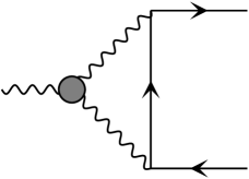
FIG. 1.: Non-SM corrections to the $Zbb$ and $\gamma bb$ vertex. The new physics enters through the ‘blob’ vertex.

In order to avoid a conflict with existing notation found in the references, but at the same time wishing to avoid a lengthy discussion of vertex corrections, two new parameters, $\Delta\Gamma_{\gamma bb}^{\rm NP}(q^{2})$ and $\Delta\Gamma_{Zbb}^{\rm NP}(q^{2})$ are introduced. (The superscript ‘NP’ indicates new physics.) They are defined according to how they modify the SM Feynman rules:

$$-i\hat{e}\gamma^{\mu}\bigg{\{}Q_{b}P_{+}+\Big{[}\Delta\Gamma_{\gamma bb}^{\rm NP}(q^{2})I_{3}+Q_{b}\Big{]}P_{-}\bigg{\}} \;,$$ (17)

$$-i\hat{g}_{Z}\gamma^{\mu}\bigg{\{}-\hat{s}^{2}Q_{b}P_{+}+\Big{[}\big{(}1+\Delta\Gamma_{Zbb}^{\rm NP}(q^{2})\big{)}I_{3}-\hat{s}^{2}Q_{b}\Big{]}P_{-}\bigg{\}} \;,$$ (18)

for the $\gamma bb$ and $Zbb$ vertices respectively. The one-loop contributions of the SM are not shown. The projection operators are defined by $P_{\pm}=(1\pm\gamma_{5})/2$, and $Q_{b}=-1/3$ and $I_{3}=-1/2$ are the charge and weak-isospin quantum numbers of the b quark. Also, $\Delta\Gamma_{\gamma bb}^{\rm NP}(0)=0$ by Ward identities[9] while $\Delta\Gamma_{Zbb}^{\rm NP}(q^{2})$ may contain a constant term. Both of these form factors receive contributions from ${\cal O}_{W}$ and ${\cal O}_{B}$ through a new-physics contribution to the $WW\gamma$ and $WWZ$ couplings as depicted in Fig. 1. (They receive corrections from ${\cal L}_{2}$, ${\cal L}_{3}$ and ${\cal L}_{9}$ in the nonlinear realization of SSB.) Recall that the pinch term is removed from the vertex correction form factor but included in the barred charges. An explicit calculation yields

$$\Delta\Gamma_{\gamma bb}^{\rm NP}(q^{2}) = -\frac{\hat{g}^{2}}{64\pi^{2}}\frac{m_{t}^{2}}{m_{W}^{2}}\bigg{\{}\frac{q^{2}}{m_{W}^{2}}\Delta\kappa_{\gamma}(q^{2})+6\Delta g_{1}^{\gamma}(q^{2})\bigg{\}}\log\bigg{(}\frac{\Lambda^{2}}{m_{Z}^{2}}\bigg{)}\;,$$ (20)

$$\Delta\Gamma_{Zbb}^{\rm NP}(q^{2}) = -\frac{\hat{g}^{2}}{64\pi^{2}}\frac{m_{t}^{2}}{m_{Z}^{2}}\bigg{\{}\frac{q^{2}}{m_{W}^{2}}\Delta\kappa_{Z}(q^{2})+6\Delta g_{1}^{Z}(q^{2})\bigg{\}}\log\bigg{(}\frac{\Lambda^{2}}{m_{Z}^{2}}\bigg{)}\;,$$ (21)

where $\Delta\kappa_{\gamma}=\kappa_{\gamma}-1$, $\Delta\kappa_{Z}=\kappa_{Z}-1$, $\Delta g_{1}^{\gamma}=g_{1}^{\gamma}-1$ and $\Delta g_{1}^{Z}=g_{1}^{Z}-1$. Recall that $g_{1}^{\gamma}(0)=1$. An expression equivalent to Eqn. (21) was presented in Ref. [15]. Replacing a $WWZ$ vertex in Fig. 1 with a $WW\gamma$ vertex introduces a factor of $\hat{s}/\hat{c}$ and requires the replacements $\Delta\kappa_{Z}\rightarrow\Delta\kappa_{\gamma}$ and $\Delta g_{1}^{Z}\rightarrow\Delta g_{1}^{\gamma}$. Taking into the account different overall factors in the definitions of Eqn. (1), the expression for $\Delta\Gamma_{\gamma bb}^{\rm NP}(q^{2})$ is obtained from the expression for $\Delta\Gamma_{Zbb}^{\rm NP}(q^{2})$. Explicit expressions for $\kappa_{\gamma}$, $\kappa_{Z}$, $g_{1}^{\gamma}$ and $g_{1}^{Z}$ from Eqns. (I) and Eqns. (I) may be used to obtain the appropriate form factors for the linear and nonlinear realizations of SSB respectively.

III The data

From the recent analysis of Ref. [16], the data for low-energy and $Z$-pole measurements is nicely summarized as measurements of the various charge form factors. That global analysis yielded, for measurements on the $Z$-pole,

$$\left.\begin{array}[]{l}\overline{g}_{Z}^{2}(m_{Z}^{2})=0.55557-0.00042\frac{\alpha_{s}+1.54\overline{\delta}_{b}(m_{Z}^{2})-0.1065}{0.0038}\pm 0.00061\\ \overline{s}^{2}(m_{Z}^{2})=0.23065+0.00003\frac{\alpha_{s}+1.54\overline{\delta}_{b}(m_{Z}^{2})-0.1065}{0.0038}\pm 0.00024\end{array}\right\}\makebox[5.69046pt]{}\rho_{\rm corr}=0.24\;,$$ (22)

where $\overline{\delta}_{b}(m_{Z}^{2})=\overline{\delta}_{b\;\rm SM}(m_{Z}^{2})+\Delta\Gamma_{Zbb}^{\rm NP}(m_{Z}^{2})$; the precise definition of $\overline{\delta}_{b}(q^{2})$ is found in Ref. [9]. Combining the $W$-boson mass measurement ($m_{W}=80.356\pm 0.125$ GeV) with the input parameter $G_{F}$,

$$\overline{g}_{W}^{2}(0)=0.4237\pm 0.0013\;.$$ (23)

And finally, from the low-energy data,

$$\left.\begin{array}[]{l}\overline{g}_{Z}^{2}(0)=0.5441\pm 0.0029\\ \overline{s}^{2}(0)=0.2362\pm 0.0044\end{array}\right\}\makebox[5.69046pt]{}\rho_{\rm corr}=0.70\;.$$ (24)

The implications of this data for non-Abelian gauge-boson couplings was considered in Ref. [15]. Note that the above data is insensitive to $\Delta\Gamma_{\gamma bb}^{\rm NP}(q^{2})$; because $\Delta\Gamma_{\gamma bb}^{\rm NP}(0)=0$, there is a negligible contribution at low energies, and on the $Z$-pole the effects of photon exchange are negligible. Also notice that there are no constraints on $\overline{\alpha}(q^{2})$ and $\overline{g}_{W}^{2}(q^{2})$ away from $q^{2}=0$.

Data is now available from measurements at LEP1.5 and LEP2. This has implications for the indirect constraints on new physics. In particular, there is now sensitivity to $\Delta\Gamma_{\gamma bb}^{\rm NP}(q^{2})$ and $\overline{\alpha}(q^{2})$. Additionally some of the contributions to the charge form factors run with $q^{2}$, hence measurements at different center of mass (CM) energies constrain different linear combinations of the parameters. Some of the contributions are enhanced as the CM energy increases, but unfortunately there is also a loss in statistics.

The three LEP detector collaborations have published measurements for $e^{+}e^{-}\rightarrow f\overline{f}$ where $f$ is a typical fermion for LEP1.5 energies of 130-140 GeV[17, 18, 19] and LEP2 energies of 161-172 GeV[20, 21]. The relevant measurements are summarised in Table I.

Detector	$\sqrt{s}$(GeV)	$\cal L$(pb-1)	$\sigma_{\rm had}$(pb)	$\sigma_{\mu^{+}\mu^{-}}$(pb)	$\sigma_{\tau^{+}\tau^{-}}$(pb)	$A_{\rm fb}^{\mu^{+}\mu^{-}}$	$A_{\rm fb}^{\tau^{+}\tau^{-}}$	$R_{b}$
ALEPH	130	2.9	74.2$\pm$6.2	9.6$\pm$1.9	11.8$\pm$2.3	0.65${}^{+0.16}_{-0.23}$	0.91${}^{+0.08}_{-0.20}$
ALEPH	136	2.9	57.4$\pm$4.8	7.1$\pm$1.7	5.8$\pm$1.7	0.53${}^{+0.22}_{-0.29}$	0.70${}^{+0.18}_{-0.42}$
L3	130.3	2.7	81.8$\pm$6.4	7.7$\pm$1.8	10.4$\pm$2.8	0.83${}^{+0.16}_{-0.22}$	0.65${}^{+0.15}_{-0.25}$
L3	136.3	2.3	70.5$\pm$6.2	6.1$\pm$1.7	9.4$\pm$2.8	0.92${}^{+0.08}_{-0.27}$	0.98${}^{+0.02}_{-0.23}$
L3	140.2	0.05	67$\pm$47
L3	161.3	10.9	37.3$\pm$2.3	4.59$\pm$0.86	4.6$\pm$1.1	0.59${}^{+0.14}_{-0.18}$	0.97${}^{+0.10}_{-0.25}$
L3	170.3	1.0	39.5$\pm$7.5
L3	172	10.2	28.2$\pm$2.3	3.60$\pm$0.76	4.3$\pm$1.1	0.31${}^{+0.19}_{-0.22}$	0.18${}^{+0.27}_{-0.29}$
OPAL	130.26	2.7	66$\pm$6	9.5$\pm$1.9	6.0$\pm$2.0
OPAL	136.23	2.6	60$\pm$5	11.6$\pm$2.1	7.6$\pm$2.3
OPAL	133					0.65$\pm$0.12	0.31$\pm$0.16	0.216$\pm$0.036
OPAL	140	0.04	50$\pm$36
OPAL	161.3	10.0	35.3$\pm$2.1	4.6$\pm$0.7	6.7$\pm$1.0	0.49$\pm$0.14	0.52$\pm$0.14	0.141$\pm$0.031

TABLE I.: LEP1.5 and LEP2 data from the three LEP detector collaborations. Statistical and systematic errors, where reported separately, have been combined in quadrature. OPAL entries at 133 GeV are actually the average of measurements at 130 GeV and 136 GeV.

Notice that the table is somewhat incomplete. ALEPH measurements at LEP2 energies are not yet available, and only L3 has reported measurements above 170 GeV. Only OPAL reports on measurements specific to b quarks. The results for OPAL at 133 GeV were obtained by combining data at 130 GeV and 136 GeV; no data was actually taken at 133 GeV. Whenever statistical and systematic errors were reported separately, they have been combined in quadrature before being entered into the table. The various table entries are treated as separate and independent measurements; no attempt is made to directly combine the results of the different collaborations.

A significant portion of the events above the $Z$ peak are “radiative return” events. That is, a photon is radiated which reduces the effective CM energy to $\sqrt{\hat{s}}\approx m_{Z}$. Except for the appearance of the extra radiation, such events are characteristically the same as LEP1 events on $Z$-pole. In consideration of the enormous number of $Z$ decays accumulated at LEP1, it is very reasonable to neglect $e^{+}e^{-}\rightarrow f\overline{f}\gamma$ events at LEP1.5 and LEP2 when the photon carries away a significant portion of the energy. For this reason only the exclusive modes are reported in the table.

Additionally it is interesting to anticipate what data might be available in the future. Four different data sets will be considered:

1. Fit 1: All low-energy and $Z$-pole data as summarised by Eqns. (22)-(24).

2. Fit 2: The data from Fit 1 plus the LEP1.5 and early LEP2 data summarised in Table I.

3. Fit 3: The data from Fit 2 plus an estimate of future LEP2 data. A luminosity of 125 pb^-1/year/detector is assumed for 2 detectors and 3 years. The luminosity is evenly divided between 188 GeV and 192 GeV. It is also assumed that LEP2 will obtain a measurement of $\Delta m_{W}=50$ MeV.

4. Fit 4: The data from Fit 3 plus 50 fb^-1 of data collected at a $\sqrt{s}=500$ GeV linear $e^{+}e^{-}$ and an assumed measurement of $\Delta m_{W}=20$ MeV at the TeV33.

For the future LEP2 data it the following observables were used: $\sigma(e^{+}e^{-}\rightarrow\mu^{+}\mu^{-})$, $\sigma(e^{+}e^{-}\rightarrow{\rm hadrons})$ and the forward-backward asymmetries $A^{\mu}_{FB}$, $A^{b}_{FB}$ and $A^{c}_{FB}$. In every case it was assumed that statistical errors dominate over systematic errors. For the linear collider the uncertainty in the luminosity measurement may contribute to an uncertainty in absolute rates. Therefore, the $R_{h}$ is used in place of the hadronic cross section, and $\sigma(e^{+}e^{-}\rightarrow\mu^{+}\mu^{-})$ is assigned an error of 3%.

IV Numerical studies and discussion

In all numerical studies the scale of new physics is taken to be $\Lambda=1$ TeV, and the renormalization scale is chosen to be $\mu=m_{Z}$. The one-sigma bounds on $f_{WWW}$, $f_{W}$ and $f_{B}$ are presented in Table II.

		$m_{H}=75$ GeV	$m_{H}=200$ GeV	$m_{H}=400$ GeV	$m_{H}=800$ GeV
$f_{WWW}$	Fit 1	-19$\pm$10	5$\pm$10	25$\pm$10	45$\pm$10
	Fit 2	-20$\pm$10	5$\pm$10	24$\pm$10	44$\pm$10
	Fit 3	-22$\pm$10	4$\pm$10	24$\pm$10	45$\pm$10
	Fit 4	-27$\pm$8	2$\pm$8	26$\pm$8	51$\pm$8
$f_{W}$	Fit 1	1.8$\pm$3.2	-5.0$\pm$3.7	-7.6$\pm$4.4	1.9$\pm$3.8
	Fit 2	2.1$\pm$3.2	-4.6$\pm$3.7	-7.3$\pm$4.4	2.0$\pm$3.8
	Fit 3	3.0$\pm$3.0	-4.3$\pm$3.6	-7.4$\pm$4.4	3.2$\pm$3.7
	Fit 4	6.1$\pm$2.4	-3.1$\pm$3.1	-8.0$\pm$4.3	9.2$\pm$3.4
$f_{B}$	Fit 1	-3$\pm$10	7.4$\pm$7.4	-0.5$\pm$4.0	-4.5$\pm$2.5
	Fit 2	-2$\pm$10	8.2$\pm$7.4	0.1$\pm$4.0	-4.1$\pm$2.5
	Fit 3	-1$\pm$10	7.2$\pm$6.8	-1.4$\pm$3.4	-5.1$\pm$2.2
	Fit 4	2.8$\pm$5.7	2.9$\pm$4.2	-4.1$\pm$2.1	-6.9$\pm$1.3

TABLE II.: Indirect constraints at the one-sigma level assuming $\Lambda=1$ TeV and using $\mu=m_{Z}$ for the renormalization scale. Fit 1 – Fit 4 are described in the text.

The central values for $f_{WWW}$ depend upon $m_{H}$ only through the SM $m_{H}$ contributions. On the other hand, both the central values $f_{W}$ and $f_{B}$ have a complicated dependence on $m_{H}$. Comparing Fit 2 to Fit 1, the data in Table I does not effect the magnitude of the error bars, but does lead to a small shift in the best-fit central values. Proceeding to Fit 3, the overall results for the LEP2 program are more promising. While the error bars on $f_{WWW}$ are unaffected, there is a tiny effect upon the error bars for $f_{W}$, and for $f_{B}$ the magnitude of the error bars is, in some cases, reduced by more than 10%. The improvement at a future linear collider (Fit 4) is significant for all three parameters.

In Fig. 2,

FIG. 2.: Constraints at the 95% confidence level in the $\Delta\kappa_{\gamma}$ versus $\lambda$ plane for $m_{H}=300$ GeV subject to the constraints of Eqns. I with $f_{B}=f_{W}$. The solid, dashed, dotted and dot-dashed curves correspond to Fit 1 (low-energy and $Z$-pole data), Fit 2 (LEP1.5 and early LEP2 data included), Fit 3 (LEP2 included) and Fit 4 (linear collider included) respectively. For the scale of new physics and the renormalization scale, $\Lambda=1$ TeV and $\mu=m_{Z}$ have been employed.

the best fit in the $\Delta\kappa_{\gamma}$ versus $\lambda$ plane is shown for $m_{H}=300$ GeV subject to the constraints of Eqns. I. There are three independent variables, $f_{W}$, $f_{B}$ and $f_{WWW}$. A two-dimensional projection is obtained by setting $f_{B}=f_{W}$. In Fig. 3

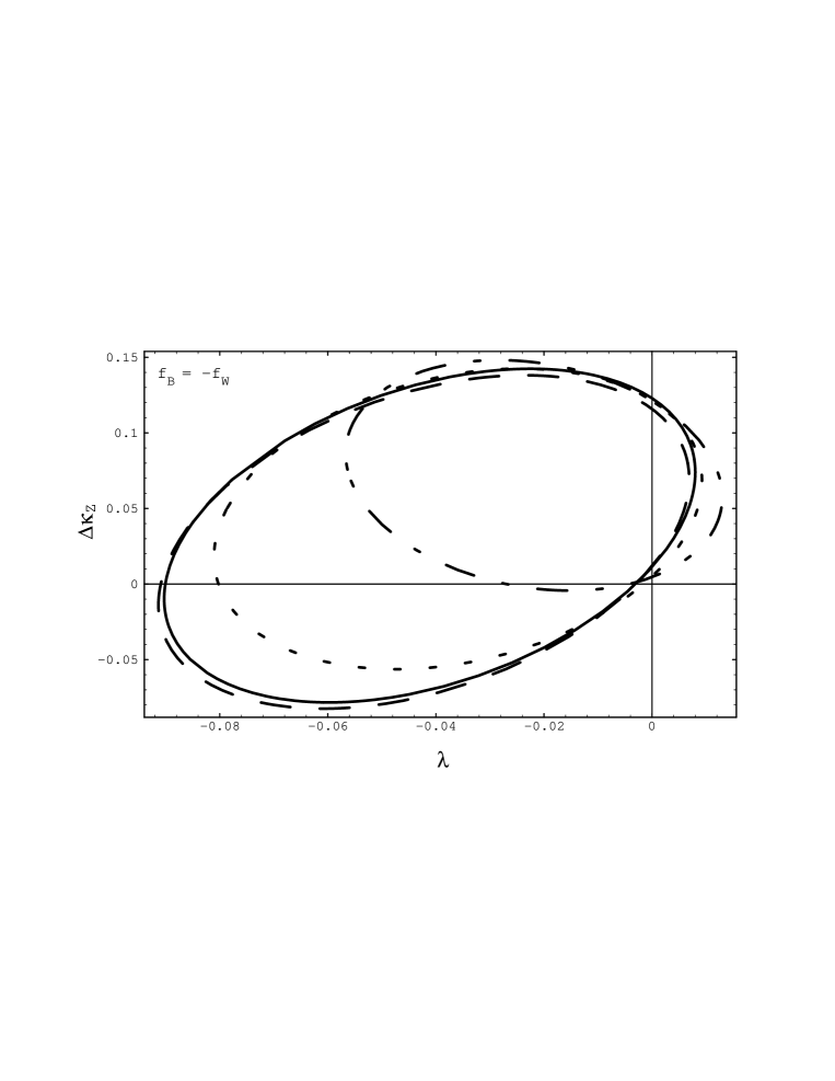
FIG. 3.: Constraints at the 95% confidence level in the $\Delta\kappa_{Z}$ versus $\lambda$ plane for $m_{H}=300$ GeV subject to the constraints of Eqns. I with $f_{B}=-f_{W}$. The solid, dashed, dotted and dot-dashed curves correspond to Fit 1 (low-energy and $Z$-pole data), Fit 2 (LEP1.5 and early LEP2 data included), Fit 3 (LEP2 included) and Fit 4 (linear collider included) respectively. For the scale of new physics and the renormalization scale, $\Lambda=1$ TeV and $\mu=m_{Z}$ have been employed.

a two dimensional projection in the $\Delta\kappa_{Z}$ versus $\lambda$ plane for $m_{H}=300$ GeV has been obtained by choosing $f_{B}=-f_{W}$ (and therefore $\Delta\kappa_{\gamma}=0$). The bounds on $\lambda$ from Figure 3 are noticeably weaker than those of Fig. 2. This illustrates an important aspect of these indirect bounds. Without restricting the discussion to a particular model, it is impossible to predict relations between the various parameters, and hence the possibility of cancellations between them must be considered. Furthermore, the central values which are obtained in the fits are sensitive to $\alpha_{s}$, the error on the hadronic contribution to the running of $\alpha_{\rm QED}$, the top-quark mass and, as shown in Table II, the unknown Higgs-boson mass. All four fits are reflected in each of these figures. Looking at the dashed curve we see that the LEP1.5 and available LEP2 data leads to only a tiny shift in the central values of the solid curves. The dotted curve reflects an important reduction in the available parameter space by the end of LEP2, and the dot-dashed curves show serious improvement at the linear collider.

These indirect bounds are particularly interesting when compared to the direct bounds which may be obtained by studying $W$-boson pair production. Such bounds, taken from Ref. [4], are summarised in Table III.

	$f_{WWW}$	$f_{W}$	$f_{B}$
LEP II	10	7.1	46
LC	0.23	0.10	0.25

TABLE III.: Direct one-sigma limits from $e^{+}e^{-}\rightarrow W^{+}W^{-}$ assuming $\Lambda=1$TeV. (From Ref. [4].) In the first row are the constraints from LEP II at 175GeV with ${\cal L}^{\rm int}=500{\rm pb}^{-1}$, and the second row contains results for a 500GeV future linear collider with ${\cal L}^{\rm int}=50{\rm fb}^{-1}$. The one-sigma allowed region is approximately symmetric about zero.

The numbers in this table make the same assumptions about a linear collider as does Fit 4. However, for LEP2, Ref. [4] considered only ${\cal L}^{\rm int}=500{\rm pb}^{-1}$ at $\sqrt{s}=175$ GeV. If the parameters in Fit 3 more accurately describe the actual LEP2 program, then the numbers in Table III are pessimistic. The errors quoted are purely statistical, and more events should be expected with more luminosity plus higher energy which tends to overcome threshold suppression factors. As discussed above, the numbers in Table II are somewhat optimistic. By the completion of LEP2, using the numbers from the tables, the ratios of the indirect to the direct bound are 1:1 for $f_{WWW}$, 1:2 for $f_{W}$ and 1:5–1:21 (depending upon $m_{H}$) for $f_{B}$. Taking into account the above discussion, it is safe to say that the direct and indirect bounds probe the same order of magnitude, and hence both studies should be optimized. Proceeding to the linear collider, the improvements in the indirect measurements are insufficient to keep pace with the improved direct measurements.

Turning to the nonlinear realization of SSB, the one-sigma bounds on $\alpha_{2}$, $\alpha_{3}$ and $\alpha_{9}$ are presented in Table table-nl-indirect.

	Fit 1	Fit 2	Fit 3	Fit 4
$\alpha_{2}$	0.252$\pm$0.053	0.250$\pm$0.053	0.261$\pm$0.051	0.211$\pm$0.037
$\alpha_{3}$	-0.119$\pm$0.023	-0.117$\pm$0.023	-0.121$\pm$0.022	-0.142$\pm$0.019
$\alpha_{9}$	-0.03$\pm$0.16	-0.03$\pm$0.16	-0.261$\pm$0.092	-0.242$\pm$0.040

TABLE IV.: Indirect constraints at the one-sigma level assuming $\Lambda=1$ TeV and using $\mu=m_{Z}$ for the renormalization scale. Fit 1 – Fit 4 are described in the text.

The inclusion of LEP1.5 and early LEP2 data (Fit 2) has a small effect on the best-fit cental values, but there is no change in the error bars. The complete LEP2 program makes a tiny reduction in the error bars for $\alpha_{2}$ and $\alpha_{3}$, but the error on $\alpha_{9}$ is reduced by 40%. At the linear collider significant improvements are achieved for $\alpha_{2}$ and $\alpha_{9}$, and the error on $\alpha_{3}$ is also reduced. As in the discussion following Table II, these bounds are weakened by correlations among the various parameters and by uncertainties in SM parameters.

The corresponding direct constraints from Ref. [4] are presented in Table V.

	$\alpha_{2}$	$\alpha_{3}$	$\alpha_{9}$
LEP II	0.34	0.053	0.10
LC	0.0018	0.00072	0.00078

TABLE V.: Direct one-sigma limits from $e^{+}e^{-}\rightarrow W^{+}W^{-}$ assuming $\Lambda=1$ TeV. (From Ref. [4].) In the first row are the constraints from LEP II at 175GeV with ${\cal L}^{\rm int}=500{\rm pb}^{-1}$, and the second row contains results for a 500GeV future linear collider with ${\cal L}^{\rm int}=50{\rm fb}^{-1}$. The one-sigma region is approximately symmetric about zero.

Again, the assumptions in obtaining these table entries are pessimistic compared to the numbers used in Fit 3. The post-LEP2 ratios of indirect to direct bounds are 1:7 for $\alpha_{2}$, 1:2.5 for $\alpha_{3}$ and 1:1 for $\alpha_{9}$. Again, the direct and indirect bounds are of the same order at LEP2. At the linear collider the direct constraints are more than an order of magnitude better than the indirect.

Finally, Fig. 4

FIG. 4.: Constraints at the 95% confidence level in the $\Delta\kappa_{\gamma}$–$\Delta\kappa_{Z}$ plane. Fig. (a) compares the linear realization of SSB (with $f_{WWW}$ = 0) for $m_{H}=100$ GeV (solid curve), $m_{H}=300$ GeV (dashed curve) and $m_{H}=700$ GeV (dotted curve) with the nonlinear realization of SSB with $\alpha_{9}=0$ (dot-dashed curve). Then, Fig. (b) and (c) specialize to $m_{H}=100$ GeV and $m_{H}=700$ GeV, respectively, and Fig. (d) concerns the nonlinear realization of SSB. In Fig. (b)-(d), the solid, dashed, dotted and dot-dashed curves correspond to Fit 1, Fit 2,Fit 3 and Fit 4 respectively. $\Lambda=1$ TeV and $\mu=m_{Z}$ have been assumed.

is a projection in the $\Delta\kappa_{\gamma}$–$\Delta\kappa_{Z}$ plane. Fig. 4(a) compares the linear realization of SSB (with $f_{WWW}$ = 0) for $m_{H}=100$ GeV (solid curve), $m_{H}=300$ GeV (dashed curve) and $m_{H}=700$ GeV (dotted curve) with the nonlinear realization of SSB with $\alpha_{9}=0$ (dot-dashed curve). Then, Fig. 4(b) and (c) specialize to $m_{H}=100$ GeV and $m_{H}=700$ GeV, respectively, and Fig. 4(d) concerns the nonlinear realization of SSB. In Fig. 4(b)-(d), the solid, dashed, dotted and dot-dashed curves correspond to Fit 1, Fit 2, Fit 3 and Fit 4 respectively. All fits are at the 95% confidence level.

Examining Fig. 4(a), the contours for the linear realization of SSB are highly dependent upon $m_{H}$, and, while all are consistent with SM, the intermediate mass of $m_{H}=300$ GeV disfavors the point $(\Delta\kappa_{\gamma},\Delta\kappa_{Z})=(0,0)$. The allowed parameter space clearly decreases with increasing $m_{H}$. On the other hand, the contour for the nonlinear realization is clearly inconsistent with the SM. Proceeding to Fig. 4(a) and (b), modest reductions in the allowed regions may be achieved at LEP2, while the improvements at the linear collider are much more significant. For the nonlinear realization of SSB, Fig. 4(d) shows minimal gains at LEP2, but the improvement at the linear collider is dramatic.

V Conclusions

Nonstandard $WW\gamma$ and $WWZ$ vertices may be probed directly via their tree-level contributions to processes such as $e^{+}e^{-}\rightarrow W^{+}W^{-}$ or indirectly via their loop-level contributions to electroweak observables. The direct constraints on these couplings will improve significantly as data is accumulated at the ongoing LEP2 experiments. The resulting direct constraints and the current indirect constraints, allowing for theoretical uncertainties in the latter, probe new physics at roughly the same level. Therefore it is desirable to also improve the indirect constraints as much as possible. The LEP1.5 and LEP2 data which is presently available leads to only a very tiny improvement, but it is anticipated that significant gains will have been accomplished before the end of the LEP2 experiments.

Truly significant improvements in the loop-level constraints are expected from the inclusion of data collected at a future linear collider operating at $\sqrt{s}=500$ GeV. However, the improvements in the direct constraints through the study of $W$-boson pair production at the same facility will be much more impressive, and it is very that the better measurements will be obtained from these direct studies.

REFERENCES

- [1] K. Hagiwara, R.D. Peccei, D. Zeppenfeld and K. Hikasa, Nucl. Phys. B282 (1987) 253.
- [2] W. Buchmüller and D. Wyler, Nucl. Phys. B268 621 (1986); C. J. C. Burgess and H. J. Schnitzer, Nucl. Phys. B228, 464 (1983); C. N. Leung, S. T. Love, and S. Rao, Z. Phys. C31, 433 (1986).
- [3] K. Hagiwara, S. Ishihara, R. Szalapski and D. Zeppenfeld, Phys. Lett. B283 (1992) 353; K. Hagiwara, S. Ishihara, R. Szalapski and D. Zeppenfeld, Phys. Rev. D48 (1993) 2182.
- [4] K. Hagiwara, T. Hatsukano, S. Ishihara and R. Szalapski, Nucl. Phys. B in press, KEK-TH-497, hep-ph/9612268.
- [5] K. Hagiwara, S. Matsumoto and R. Szalapski, Phys. Lett. B357 (1995) 411.
- [6] A.C. Longhitano, Phys. Rev. D22 (1980) 1166; A.C. Longhitano, Nucl. Phys. B188 (1981) 118; T. Appelquist and G.H. Wu, Phys. Rev. D48 (1993) 3235.
- [7] S. Dawson and G. Valencia, Phys. Lett. B333 (1994) 207-211.
- [8] F. Feruglio, Int. Journ. of Mod. Phys. A8 (1993) 4937.
- [9] K. Hagiwara, D. Haidt, C. S. Kim and S. Matsumoto, Z. Phys. C64 (1994) 559.
- [10] D.C. Kennedy and B.W. Lynn, Nucl. Phys. B322 (1989) 1.
- [11] J.M. Cornwall and J. Papavassiliou, Phys. Rev. D40 (1989) 3474; J. Papavassiliou, Phys. Rev. D41 (1990) 3179.
- [12] G. Degrassi and A. Sirlin, Nucl. Phys. B383 (1992) 73; Phys. Rev. D46 (1992) 3104; G. Degrassi, B.A. Kniehl and A. Sirlin, Phys. Rev. D48 (1993) 3963.
- [13] J. Papavassiliou and K. Philippides, Phys. Rev. D48 (1993) 4255; J. Papavassiliou and A. Sirlin, Phys. Rev. D50 (1994) 5951; J. Papavassiliou, Phys. Rev. D50 (1994) 5958; J. Papavassiliou and K. Philippides, Phys. Rev. D52 (1995) 2355; J. Papavassiliou, (Feb. 1995) hep-ph-9504382; J. Papavassiliou and A. Pilaftsis, Phys. Rev. Lett. 75 (1995) 3060.
- [14] S. Dawson and G. Valencia, Nucl. Phys. B439 (1995) 3-22.
- [15] S. Alam, S. Dawson and R. Szalapski, KEK-TH-519, KEK Preprint 97-88, BNL-HET-SD-97-003, hep-ph/9706542.
- [16] K. Hagiwara, D. Haidt and S. Matsumoto, KEK-TH-512, DESY 96-192, hep-ph/9706331, for publication in Z. Phys. C.
- [17] ALEPH Collaboration, Phys. Lett. B378 (1996) 373-384.
- [18] L3 Collaboration, Phys. Lett. 370 (1996) 195-210.
- [19] OPAL Collaboration, Phys. Lett. B376 (1996) 232-244.
- [20] OPAL Collaboration, Phys. Lett. B391 (1997) 221-234.
- [21] L3 Collaboration, CERN-PPE/97-52, 7 May 1997.