On-Shell Approach to Pion-Nucleon Physics

Abstract

We discuss an on-shell approach to pion-nucleon physics that is consistent order by order in a $1/f_{\pi}$ expansion with the chiral reduction formula, crossing, and relativistic unitarity. A number of constraints between the on-shell low-energy parameters are derived at tree level in the presence of the pion-nucleon sigma term, and found to be in fair agreement with experiment. We analyze the nucleon form factors, and the $\pi N\to\pi N$ scattering amplitude to one-loop, as well as $\pi N\to\pi\pi N$ to tree level. We use the latter to derive a new constraint for the pion-nucleon sigma term at threshold. We compare our results to both relativistic and non-relativistic chiral perturbation theory, and discuss the convergence character of the expansion in light of experiment.

I Introduction

Pion-nucleon interactions have been extensively investigated using dispersion relations and chiral symmetry. Most of these studies are built around unphysical points such as the soft pion limit [1] or the chiral limit [2]. A typical example is the pion-nucleon sigma term — the fraction of the nucleon mass due to the explicit breaking of chiral $SU(2)\times SU(2)$. The scattering amplitude is analytically continued to the unphysical Cheng-Dashen point [3], and chiral perturbation theory (ChPT) is applied [4].

An important exception to the above is Weinberg’s on-shell formula for pion-nucleon scattering [5], which also yields the Tomozawa-Weinberg relations for the S-wave scattering lengths [6]. Recently, we have been able to extend this result to processes involving an arbitrary number of on-shell pions and nucleons [7]. A number of identities using the chiral reduction formula were derived — one of which was applied to $\pi\pi$ scattering and shown to be in good agreement with the data well beyond threshold [8].

This paper applies the results of the chiral reduction formula to the nucleon sector, allowing for an on-shell determination of the pion-nucleon sigma term and $\pi N$ scattering. We start by introducing a model in section II that is uniquely specified by the form of the symmetry breaking in QCD to tree level. This model can be used to ensure Lorentz invariance, causality, and positivity while at the same time enforce the constraints brought about by the chiral reduction formula. The strategy involved in this calculation compared to those of ChPT is presented in section III. In section IV, we derive an axial Ward identity and discuss the deviation from the Goldberger-Treiman relation. In section V, we recall Weinberg’s relation for $\pi N$ scattering and use the measured S-wave scattering lengths to predict the pion-nucleon sigma term, the pion-nucleon coupling, and the induced pseudoscalar coupling to tree level. In section VI, we discuss the one-loop on-shell corrections to the vector, axial, and scalar form factors, and critically examine the character of the convergence. We then evaluate the one-loop corrections to $\pi N$ scattering in section VII. Finally, we look at $\pi N\to\pi\pi N$ to tree level and find an additional way to determine the pion-nucleon sigma term in section VIII. Our conclusions are summarized in section IX. Details about the Feynman rules and the loop expansion are found in the appendices.

II Model

There are two kinds of chiral models possible for the $\pi N$ system. The first is a Skyrme-type model, where the nucleon is a chiral soliton [9]. Since solitons often accompany spontaneous symmetry breaking, this is a natural approach. Also, if vector mesons (particularly the omega) are included in chiral Lagrangians, avoiding soliton solutions is more difficult than having them.

However, there are two difficulties in this model. One is that the semiclassical expansion does not commute with the chiral limit. As a result, the S-wave $\pi N$ scattering lengths are not compatible with the Tomozawa-Weinberg relation to leading order [10]. Similarly, the nucleon axial charge $g_{A}$ is small to leading order (about half of experiment), and yields a different sign for $g_{A}-1$ [10] from that obtained with the Adler-Weisberger sum rule. This means that a quantitative comparison with experiment is usually difficult, unless a calculational scheme beyond the semiclassical expansion is developed.

The other difficulty is more fundamental. In QCD, nucleon operators $qqq$ and meson operators $\overline{q}q$ exist, which are mutually local. This has not been shown in Skyrme-type models [11].

We will therefore adopt the other type of model, where pions and nucleons are taken to be independent. For the $SU(2)\times SU(2)$ symmetric part of $\pi N$ interactions, we take the standard non-linear sigma model as the effective Lagrangian gauged with vector and axial-vector external sources.

$${\cal L}_{1} = \frac{f_{\pi}^{2}}{4}{\rm Tr}\left[\left(iD_{\mu}U+\left\{\hat{a}_{\mu},U\right\}\right)\left((iD^{\mu}U)^{\dagger}+\left\{\hat{a}^{\mu},U^{\dagger}\right\}\right)\right]$$ (4)

$$+{\overline{\bf\Psi}}\left(i\hbox to0.0pt{/\hss}\partial+\hbox to0.0pt{/\hss}{\hat{v}}+\hbox to0.0pt{/\hss}{\hat{a}}\gamma_{5}\right){\bf\Psi}-m_{0}\left(\overline{\bf\Psi}_{R}U{\bf\Psi}_{L}+\overline{\bf\Psi}_{L}U^{\dagger}{\bf\Psi}_{R}\right)$$

$$+\frac{1}{2}(g_{A}-1)\overline{\bf\Psi}_{R}\left(i\,\raise 0.6458pt\hbox{$/$}\kern-7.20001pt\hbox{$D$}U+\left\{\hbox to0.0pt{/\hss}{\hat{a}},U\right\}\right)U^{\dagger}{\bf\Psi}_{R}$$

$$-\frac{1}{2}(g_{A}-1)\overline{\bf\Psi}_{L}U^{\dagger}\left(i\,\raise 0.6458pt\hbox{$/$}\kern-7.20001pt\hbox{$D$}U+\left\{\hbox to0.0pt{/\hss}{\hat{a}},U\right\}\right){\bf\Psi}_{L}$$

where $U$ is a chiral field, ${\bf\Psi}=({\bf\Psi}_{R},{\bf\Psi}_{L})$ is the nucleon field, $\hbox to0.0pt{/\hss}\partial=\gamma^{\mu}\partial_{\mu}$, ${\hat{v}}_{\mu}=v_{\mu}^{a}\tau^{a}/2$, and $D_{\mu}U=\partial_{\mu}U-i[{\hat{v}}_{\mu},U]$. In the low-energy limit, matrix elements calculated from (4) are essentially unique, given that the isospin of the nucleon is $\frac{1}{2}$ [12]. Higher derivative (1,1) terms at tree level lead to pathologies such as acausality or lack of positivity, so they will not be considered.

Ignoring isospin breaking and strong CP violation, the term which explicitly breaks chiral symmetry must be a scalar-isoscalar. The simplest non-trivial representation of $SU(2)\times SU(2)$ which contains such a term is $(2,2)$. This is the same representation as the quark mass term $\hat{m}\overline{q}q$ in QCD which generates both the pion mass and the sigma term. Therefore we take

$${\cal L}_{2} = \frac{1}{4}f_{\pi}^{2}m_{\pi}^{2}\,{\rm Tr}\left(U+U^{\dagger}\right)-\frac{m_{\pi}^{2}}{\Lambda}\,\overline{\bf\Psi}{\bf\Psi}$$ (6)

$${}-c\frac{m_{\pi}^{2}}{4\Lambda}\,{\rm Tr}\left(U+U^{\dagger}\right)\overline{\bf\Psi}_{R}U{\bf\Psi}_{L}+h.c.$$

with $c$ and $\Lambda$ arbitrary constants. A bilinear form in ${\bf\Psi}$ in (6) has been retained, again in analogy with $\hat{m}\overline{q}q$. We assume that $\Lambda$ is non-vanishing as $m_{\pi}\rightarrow 0$, so that (6) vanishes in the chiral limit. Scalar and pseudoscalar external fields can be added to eq. (6) by taking

$$m_{\pi}^{2}{\rm Tr}\,U\to{\rm Tr}\left[(m_{\pi}^{2}+s-i\tau^{a}p^{a})U\right]$$

$$m_{\pi}^{2}\overline{\bf\Psi}{\bf\Psi}\to{\overline{\bf\Psi}}(m_{\pi}^{2}+s-i\tau^{a}p^{a}\gamma_{5}){\bf\Psi}$$

and similarly for ${\rm Tr}\,U^{\dagger}$. The nucleon mass is defined as $m_{N}\equiv m_{0}+\sigma_{\pi N}$ with the pion-nucleon sigma term $\sigma_{\pi N}=(1+c)m_{\pi}^{2}/\Lambda$ as read from the Lagrangian to tree level.

Noether’s theorem implies that the symmetry breaking term must be non-derivative, otherwise the vector and axial vector currents will not transform as $(3,1)+(1,3)$. The only other term allowable in the $(2,2)$ representation then is $\overline{\bf\Psi}_{R}U^{2}{\bf\Psi}_{L}+h.c.$ which is a linear combination of the terms already included in eq. (6). Therefore our starting point for the loop-expansion ${\cal L}_{1+2}$ is essentially unique.

The currents used in this paper can be written down by functional differentiation of the action ${\bf I}\equiv\int\!d^{4}x\,{\cal L}_{1+2}$ with respect to the external sources. In particular, the pion field is just

$$\pi^{a}(x) = \frac{1}{f_{\pi}}\frac{\delta{\bf I}}{\delta p^{a}(x)}$$ (7)

$$= -i\frac{f_{\pi}}{4}{\rm Tr}\left(\tau^{a}(U-U^{\dagger})\right)+\frac{1}{f_{\pi}\Lambda}\overline{\bf\Psi}i\gamma_{5}\tau^{a}{\bf\Psi}$$ (9)

$${}+i\frac{c}{4f_{\pi}\Lambda}{\rm Tr}\left(\tau^{a}(U-U^{\dagger})\right)\overline{\bf\Psi}_{R}U{\bf\Psi}_{L}+h.c.$$

which reduces to the free incoming pion field $\pi_{\rm in}(x)$ as $x_{0}\to-\infty$. This choice is just the gauge covariant version of the PCAC pion field, also defined in terms of the axial current ${\bf A}_{\mu}^{a}\equiv\delta{\bf I}/\delta a_{\mu}^{a}$ as $\partial^{\mu}{\bf A}^{a}_{\mu}=f_{\pi}m_{\pi}^{2}\pi^{a}$.

The one-pion reduced axial current can be defined as the part of the full axial current that contains no $\pi_{\rm in}$ part. The most convenient definition is

$${\bf j}_{A\mu}^{a} = {\bf A}_{\mu}^{a}+f_{\pi}\partial_{\mu}{\pi}^{a}$$ (10)

$$= g_{A}\overline{\bf\Psi}\gamma_{\mu}\gamma_{5}\frac{\tau^{a}}{2}{\bf\Psi}+\frac{1}{\Lambda}\partial_{\mu}\left(\overline{\bf\Psi}i\gamma_{5}\,\tau^{a}{\bf\Psi}\right)$$ (12)

$${}-\frac{c}{f_{\pi}\Lambda}\partial_{\mu}\left(\pi^{a}\overline{\bf\Psi}{\bf\Psi}\right)+{\cal O}(\pi^{3}).$$

with the expansion to leading order in the PCAC pion field given in the last two lines. We note that the PCAC pion field is uniquely defined off-shell within the prescriptions of [7], and so is ${\bf j}_{A\mu}$. The vector ${\bf V}_{\mu}^{a}$ and scalar $\sigma$ currents are similarly defined through

$${\bf V}^{a}_{\mu}(x) = i\frac{f_{\pi}^{2}}{8}{\rm Tr}\left([\tau^{a},U^{\dagger}]\partial_{\mu}U\right)+h.c.+\overline{\bf\Psi}\gamma_{\mu}\frac{\tau^{a}}{2}{\bf\Psi}$$

$${}-\frac{1}{4}(g_{A}-1)\overline{\bf\Psi}_{L}\gamma_{\mu}U^{\dagger}[\tau^{a},U]{\bf\Psi}_{L}$$

$${}+\frac{1}{4}(g_{A}-1)\overline{\bf\Psi}_{R}\gamma_{\mu}[\tau^{a},U]U^{\dagger}{\bf\Psi}_{R}$$

$$\sigma(x) = \frac{1}{m_{\pi}^{2}f_{\pi}}\,{\cal L}_{2}\,.$$

The Feynman rules for ${\cal L}_{1+2}$ that are used throughout this paper are in Appendix A.

III Strategy

We adopt an on-shell loop expansion in $1/f_{\pi}$ which can be thought of as a semi-classical expansion with $\sqrt{\hbar}\sim 1/f_{\pi}$. It includes pions and nucleon loops beyond tree-level, and is consistent order by order with the identities following from the chiral reduction formula. This expansion applies equally well to the non-linear sigma-model and QCD as thoroughly discussed in [7]. We recall that in both cases, the physical pion decay constant $f_{\pi}$ shows up through the asymptotic condition of PCAC on the axial-vector current. Therefore, it is a good expansion parameter when the master formula approach is applied to these two cases.

All scattering amplitudes will be reduced by the identities derived in [7], and then expanded to one-loop using the Feynman diagrams from (4-6). This way, reparameterization invariance (in the sense of Nishijima-Gursey [14]) and vector as well as axial-vector current identities are guaranteed to one-loop. If we were to just use (4-6) without the chiral reduction formula, then $\pi\pi$ scattering subdiagrams in, for example $\pi N\rightarrow\pi N$ or $\pi N\rightarrow\pi\pi N$ appear to break reparameterization invariance. In [7] we have checked that conventional ChPT fulfills the pertinent identities following from the chiral reduction formula in the mesonic sector. We are not aware of such checks in the nucleon sector. This work and others to follow will provide for these checks in our approach.

In our approach broken chiral symmetry and relativistic unitarity will be addressed for each process individually directly on-shell. This procedure is conceptually clear, since on-shell renormalization implies that quantities $m_{N}$, $g_{A}$, $\Lambda$, $\sigma_{\pi N}$, $f_{\pi}$, and $m_{\pi}$ are fixed once and for all at tree level, thereby including all powers of the quark masses and QCD scale. (In constrast to ChPT where the chiral logarithms are assessed in these quantities.)

The ultraviolet finite and non-diagrammatic formulation extensively discussed in [7] will be presented elsewhere [15]. To make our exposition in line with current expositions using ChPT, we will use diagrams. A BPHZ (momentum) subtraction scheme will be used throughout. This is to enforce the number of subtraction constants commensurate with the number of divergences. Dimensional regularization is not appropriate, since we need to evaluate nucleon loops in the axial form factors. These are in general quadratically divergent, requiring two subtraction constants as opposed to one by dimensional regularization.

Our strategy is essentially the same as for ordinary renormalizable theories. No constants other than those required by the divergences will be considered. This makes our approach minimal in comparison to ChPT where all possible constants required by symmetry and power counting are used. This is appealing in that less constants need to be fixed. Although ChPT is more general (and generalized ChPT [16] even more so), the excess of constants there require additional assumptions such as resonance saturation [17] to fix them. In any case, which is the better approach will be dictated by comparison with experiment.

Below, we will show that to one-loop our results for the form factors reduce to those obtained by Gasser, Sainio and Švarc [4] (GSS) in the context of relativistic chiral perturbation theory when the nucleon is taken off mass shell ($\Lambda\to\infty$). On mass shell, however, a number of relations are already observed at tree level in reasonable agreement with experiment, emphasizing the importance of (broken) chiral symmetry. What is undoubtedly important in our approach is that the pion-nucleon sigma term is included at tree level along with the pion mass term. Since both terms originate from the same quark mass term in QCD, they naturally go together. This term — along with the on-shell renormalization scheme — allow the pions and nucleons to stay on mass shell to all orders. A nonzero nucleon scalar form factor and Goldberger-Treiman discrepancy at tree level are also consequences of this.

Finally, as is well known, the loop expansion in the pionic sector is equivalent to a momentum expansion [4]. This is no longer true in the pion-nucleon sector. To overcome this, heavy baryon chiral perturbation theory (HBChPT) was proposed [18], where an expansion in $1/m_{N}$ is made [19, 20]. However, the relativistic one-loop calculations contain terms which behave as ${\rm ln}\,m_{\pi}/m_{N}$ and are not able to be expanded in this way. Also in this limit relativistic unitarity is lost, making comparison with experiments difficult. Lacking a satisfactory theoretical resolution of these issues, we will maintain a relativistic approach throughout. Comparison with HBChPT will be made directly by expanding the on-shell results.

At this point we note that the unitarity bounds are more stringent than simple power counting based on a momentum expansion. For instance in $\pi\pi$ scattering the unitarity bound is saturated for $k^{2}\leq 5.2m_{\pi}^{2}$ whereas in $\pi N$ scattering the bound is $k^{2}\leq 3.8m_{\pi}^{2}$, indicating in both cases that the expansion parameter should in fact be closer to $k^{2}/4\pi f_{\pi}^{2}$ instead of $k^{2}/(4\pi)^{2}f_{\pi}^{2}$. Throughout, we will work in the kinematical regime where tree contributions are greater than one-loop, but within the unitary bounds. All the loop corrections discussed in this work are on the order of $10-30\%$ of the tree level result with the exception of the $1/\Lambda$ terms which are small enough to be sensitive to the input parameters. These terms will be assessed in as many ways as possible.

IV Axial Ward Identity

The matrix element of the axial-vector current between nucleon states of momentum $p_{i}$ and implicit spin dependence $s_{i}$ can be decomposed as

$$\langle N(p_{2})|{\bf j}^{a}_{A\mu}(0)|N(p_{1})\rangle=$$ (13)

$$=\overline{u}(p_{2})\left(\gamma_{\mu}\gamma_{5}\,G_{1}(t)+(p_{2}-p_{1})_{\mu}\gamma_{5}\,\overline{G}_{2}(t)\right)\frac{\tau^{a}}{2}\,\,u(p_{1})$$ (14)

with $t=(p_{1}-p_{2})^{2}$ and $G_{1}$ and $\overline{G}_{2}$ are free of pion poles. From (9-10), we also have $\partial^{\mu}{\bf j}_{A\mu}=f_{\pi}(\Box+m_{\pi}^{2})\,\pi$. Hence,

$$\langle N(p_{2})|\pi^{a}(0)|N(p_{1})\rangle=$$ (15)

$$=\frac{1}{f_{\pi}}\frac{1}{m_{\pi}^{2}-t}\left(2m_{N}\,G_{1}(t)+t\,\overline{G}_{2}(t)\right)\overline{u}(p_{2})i\gamma_{5}\,\frac{\tau^{a}}{2}\,\,u(p_{1})$$ (16)

By definition, eq. (16) is also equal to

$$g_{\pi NN}(t)\frac{1}{m_{\pi}^{2}-t}\overline{u}(p_{2})i\gamma_{5}\tau^{a}u(p_{1})$$

and leads to the following Ward identity

$$f_{\pi}g_{\pi NN}(t)=m_{N}G_{1}(t)+\frac{t}{2}\overline{G}_{2}(t)$$ (17)

where $g_{\pi NN}=g_{\pi NN}(m_{\pi}^{2})$ is the pion-nucleon coupling constant. Extrapolating from $t=m_{\pi}^{2}$ to $t=0$ gives the standard Goldberger-Treiman relation $g_{A}m_{N}\sim f_{\pi}g_{\pi NN}$, with $G_{1}(0)\equiv g_{A}$.

Relation (17) is exact. The Goldberger-Treiman discrepancy is just given by

$\displaystyle f_{\pi}\left(g_{\pi NN}(m_{\pi}^{2})-g_{\pi NN}(0)\right)\equiv-\overline{\Delta}_{\pi N}$

We stress again that $g_{\pi NN}(t)$ is physically accessible at both $t=m_{\pi}^{2}$ and $t=0$, making the above discrepancy measurable. Substituting (10) at tree level into (14) gives $G_{1}(t)=g_{A}$ and $\overline{G}_{2}(t)=-2/\Lambda$. Therefore using (17) we find $\overline{\Delta}_{\pi N}=m_{\pi}^{2}/\Lambda$ to tree level. We choose to renormalize $\Lambda$ on-shell such that this is true to all orders in the loop expansion. So

$$f_{\pi}g_{\pi NN}=g_{A}m_{N}-\frac{m_{\pi}^{2}}{\Lambda}\equiv G$$ (18)

and $m_{\pi}^{2}/\Lambda$ is exactly the Goldberger-Treiman discrepancy.

V Weinberg’s Relation

One way to determine $G$ and therefore attain a value for $g_{\pi NN}$ is to use pion-nucleon scattering at threshold. The scattering amplitude $i{\cal T}$ fulfills a basic Ward identity established by Weinberg [5] and reproduced by the master formula approach [7]. Taking $(k_{1},a)$ as the incoming pion, and $(k_{2},b)$ as the outgoing pion, with $p_{1}+k_{1}=p_{2}+k_{2}$, the formula is

$$i{\cal T}=i{\cal T}_{V}+i{\cal T}_{S}+i{\cal T}_{AA}$$

$$i{\cal T}_{V} = -\frac{1}{f_{\pi}^{2}}k_{1}^{\mu}\epsilon^{bac}\langle N(p_{2})|{\bf V}_{\mu}^{c}(0)|N(p_{1})\rangle_{\rm conn.}$$

$$i{\cal T}_{S} = -\frac{i}{f_{\pi}}m_{\pi}^{2}\delta^{ab}\langle N(p_{2})|{\sigma}(0)|N(p_{1})\rangle_{\rm conn.}$$

$$i{\cal T}_{AA} = -\frac{1}{f_{\pi}^{2}}k_{1}^{\mu}k_{2}^{\nu}\int\!d^{4}x\;e^{-ik_{1}\cdot x}$$

$$\times\langle N(p_{2})|T^{*}{\bf j}_{A\mu}^{a}(x){\bf j}_{A\nu}^{b}(0)|N(p_{1})\rangle_{\rm conn.}\,\,.$$

The isospin structure is decomposed as ${\cal T}^{ba}=\delta^{ab}{\cal T}^{+}+i\epsilon^{bac}\tau^{c}{\cal T}^{-}$ to give

$${\cal T}^{+}={\cal T}_{S}^{+}+{\cal T}_{AA}^{+}\qquad\qquad{\cal T}^{-}={\cal T}_{V}^{-}+{\cal T}_{AA}^{-}.$$

The amplitudes ${\cal T}^{\pm}$ can be calculated to tree level using the Feynman rules in Appendix A. At threshold they are

$${\cal T}^{+}=\frac{\sigma_{\pi N}}{f_{\pi}^{2}}-\frac{\overline{\Delta}_{\pi N}^{2}}{f_{\pi}^{2}m_{N}}-\frac{G^{2}}{f_{\pi}^{2}}\frac{m_{\pi}^{2}/m_{N}}{4m_{N}^{2}-m_{\pi}^{2}}$$ (19)

$${\cal T}^{-}=\frac{m_{\pi}}{2f_{\pi}^{2}}\left(1-g_{A}^{2}\right)+\frac{G^{2}}{f_{\pi}^{2}}\frac{2m_{\pi}}{4m_{N}^{2}-m_{\pi}^{2}}.$$ (20)

Here the pion-nucleon sigma term $\sigma_{\pi N}$ and the Goldberger-Treiman discrepancy $\overline{\Delta}_{\pi N}$ appear. These expressions reduce to the Tomozawa-Weinberg formulas for $\Lambda\to\infty$, showing the corrections are small.

Experimentally, the threshold amplitudes are expressed in terms of the S-wave scattering lengths ${\cal T}^{\pm}=4\pi(1+m_{\pi}/m_{N})a^{\pm}$. The Karlsruhe-Helsinki phase shift analysis gives $(a^{-},a^{+})=(9.2\pm 0.2,-0.8\pm 0.4)\times 10^{-2}/m_{\pi}$ [21]. The same group now has new data from PSI [22] which reduces many of the inconsistencies for low pion energies and finds a positive value $a^{+}=0$ — $4\times 10^{-3}/m_{\pi}$. Furthermore, pionic atoms give $a^{+}=2\pm 1\times 10^{-3}/m_{\pi}$ [23]. Therefore we take the weighted mean $a^{+}=1.5(9)\times 10^{-3}/m_{\pi}$. The accuracy of $a^{-}$ is less of an issue, so we will take the value given above. These give $\overline{\Delta}_{\pi N}=-54\pm 10$ MeV and $\sigma_{\pi N}=14\pm 1$ MeV. Using eq. (18), this value of $G$ gives $g_{\pi NN}=13.45\pm 0.15$, very close to the experimental value $13.4$ taken in the Paris and Bonn potentials [24]. Our on-shell tree level calculation favors a positive value for $a^{+}$ and smaller than normal value for $\sigma_{\pi N}$. This is opposite to what [25] finds, meriting a one-loop evaluation as carried out in section VII.

We can also determine the value for the induced pseudoscalar coupling constant which has been experimentally measured by two groups

$\displaystyle g_{p}\equiv m_{\mu}G_{2}(-0.88m_{\mu}^{2})=\left\{\displaystyle 8.2\pm 2.4\;\;\;\mbox{ref. \cite[cite]{[\@@bibref{Number}{CAPTURE}{}{}]}}\atop\displaystyle 8.7\pm 1.9\;\;\;\mbox{ref. \cite[cite]{[\@@bibref{Number}{CAPTURE2}{}{}]}}\right.$

from muon capture in hydrogen. Using eq. (10-16) and the definition of $G_{2}$ from the full-axial vector current

$$\langle N(p_{2})|{\bf A}^{a}_{\mu}(0)|N(p_{1})\rangle=$$

$$=\overline{u}(p_{2})\left(\gamma_{\mu}\gamma_{5}G_{1}(t)+(p_{2}-p_{1})_{\mu}\gamma_{5}G_{2}(t)\right)\frac{\tau^{a}}{2}u(p_{1})$$

gives a relation between $G_{2}$ and $\overline{G}_{2}$

$$G_{2}(t)=\frac{1}{m_{\pi}^{2}-t}\left(2m_{N}G_{1}(t)+m_{\pi}^{2}\overline{G}_{2}(t)\right).$$ (21)

Using eq. (18) we find to tree level

$\displaystyle g_{p}=\frac{2m_{\mu}G}{m_{\pi}^{2}+0.88m_{\mu}^{2}}\simeq 9.0$

which is at most $10\%$ higher than the experimental value.

VI Form Factors

We now calculate the vector form factor in order to gain insight into the loop corrections. It can be decomposed as

$$\langle N(p_{2})|{\bf V}_{\mu}^{a}(0)|N(p_{1})\rangle=$$

$$=\overline{u}(p_{2})\left(\gamma_{\mu}F_{1}(t)+\frac{i}{2m_{N}}\sigma_{\mu\nu}(p_{2}-p_{1})^{\nu}F_{2}(t)\right)\frac{\tau^{a}}{2}u(p_{1})$$

The tree level result just gives the charge $F_{1}(t)=1$. Including the one-loop form of the vector current, we find

$$F_{1}(t)=1+\frac{2(g_{A}^{2}-1)}{f_{\pi}^{2}}\left(tc^{V}_{2}+\overline{\overline{J^{\pi\pi}_{22}}}(t)\right)$$

$${}+\frac{G^{2}}{f_{\pi}^{2}}\Bigg{[}2\overline{\Gamma^{\pi N}_{3}}(t)-\overline{J^{NN}}(t)+8\overline{\Gamma^{N\pi}_{3}}(t)-m_{\pi}^{2}\overline{\Gamma^{\pi N}}(t)$$

$${}+8m_{N}^{2}\left(\overline{\Gamma^{\pi N}_{4}}(t)+4\overline{\Gamma^{N\pi}_{4}}(t)-4\overline{\Gamma^{N\pi}_{1}}(t)+\overline{\Gamma^{N\pi}}(t)\right)\Bigg{]}$$

$$F_{2}(t)=-\frac{8m_{N}^{2}G^{2}}{f_{\pi}^{2}}\left[\Gamma^{\pi N}_{4}(t)+\Gamma^{N\pi}(t)+4\Gamma^{N\pi}_{4}(t)-4\Gamma^{N\pi}_{1}(t)\right]$$

with the $\Gamma$’s representing loop integrals defined in Appendix A and $G=g_{A}m_{N}-m_{\pi}^{2}/\Lambda$ as in the previous section. An overlined function denotes a subtraction at $t=0$. Other than the subtraction constants, this reduces to the ChPT result of GSS for $\Lambda\to\infty$. This is to be expected from the form of the Lagrangian used and is a good check on the calculation. Notice that the coefficients of the terms group into factors of $G/f_{\pi}\equiv g_{\pi NN}$ to the order we are calculating by eq. (18).

Another check is that the charge $F_{1}(0)=1$ is not renormalized by loop corrections from the strong force. This can be shown to be true in dimensional regularization [4]. However, for the rest of this paper we will instead adopt the BPHZ renormalization scheme. This just amounts to subtracting the Taylor series of divergent loop integrals up to the degree of divergence and replacing the subtraction by arbitrary constants. This has two advantages: 1) we do not need to construct the most general Lagrangian to obtain the constants, 2) we obtain only the minimal amount of constants consistent with the symmetries of the theory. In other words, if a diagram is not divergent, we do not do any subtractions on it.

The only constant to one-loop, $c^{V}_{2}$, can be fixed by the vector charge radius of the nucleon $\langle r^{2}\rangle^{V}_{1}=6F_{1}^{\prime}(0)=0.578$ fm² [28] giving $2(g_{A}^{2}-1)c^{V}_{2}=7.30\times 10^{-3}$. This accounts for about one third of the radius with the rest being given by the loop integrals. This also agrees with ChPT.

The first difference with ChPT is that there is no subtraction constant for the Pauli form factor $F_{2}$. In fact, the experimental value for $F_{2}(0)$ is just the difference in the anomalous magnetic moments $\kappa_{p}-\kappa_{n}\equiv\kappa_{v}=3.71$; and a numerical calculation shows this is indeed valid to about $3\%$ as first shown by GSS. The most general Lagrangian, however, allows an extra subtraction constant for $F_{2}$ which is not needed [4].

We can also check the consistency of our results with those of heavy baryon chiral perturbation theory by taking $\Lambda\to\infty$ and expanding in $m_{\pi}/m_{N}$ and $t/m_{N}^{2}$. The consistency of the finite parts of the vector form factor with the relativistic theory has been shown by [19]. However, the opening of the two pion threshold at $t=4m_{\pi}^{2}$ which is also seen in the data for the vector form factor [28] is lost in HBChPT. In addition, extra divergences in the $1/m_{N}$ expansion can develop. If these divergences cannot be absorbed into the already existing divergence structure, the procedure of taking the limit of a large nucleon mass at the level of the Lagrangian could be different than taking this limit after calculating all amplitudes with a finite nucleon mass.

One such case does occur in the slope of the Pauli form factor $F_{2}(t)$. The full one-loop calculation can be worked out from the explicit form of the loop integrals in Appendix A to give ($\mu=m_{\pi}/m_{N}$)

$$F_{2}^{\prime}(0)=\frac{G^{2}}{3(4\pi f_{\pi})^{2}}\int_{0}^{1}\!\!dy\;\frac{y^{3}\left[y^{2}+4(1-y)^{2}\right]}{\left[y^{2}+\mu^{2}(1-y)\right]^{2}}$$

$$=\frac{G^{2}}{(4\pi f_{\pi})^{2}m_{N}^{2}}\left(\frac{\pi}{3\mu}+2\ln\mu^{2}+\frac{29}{6}\right)+{\cal O}\!(\mu).$$

which is consistent with GSS in the $\Lambda\to\infty$ limit. The $\ln\mu^{2}$ cannot be expanded in $1/m_{N}$. In principle, this should be taken into account in HBChPT by an additional subtraction constant.

Taking $g_{A}=1.265$ and $\overline{\Delta}_{\pi N}=-54$ MeV as in the last section, the magnetic radius $\langle r^{2}\rangle_{2}^{V}=6F_{2}^{\prime}(0)/\kappa_{v}$ is $0.21$ fm² to one-loop. The terms to ${\cal O}(1)$ give $0.31$ fm² and the $1/\mu$ term alone gives the HBChPT result of $0.51$ fm². The empirical value is $0.77$ fm² [28]. Ironically, the first term in the $\mu$ expansion gives the result closest to experiment. However, this term can only be singled out in a non-relativistic expansion which then would require the additional subtraction constant to absorb the logarithmic singularities mentioned above.

There are no corrections of order $m_{N}^{2}/(4\pi f_{\pi})^{2}$ to $F_{1}(0)$ since it is protected by a non-renormalization condition. In addition, $F_{2}(0)$ had no contribution from tree level and the one-loop value was shown to be close to the experimental value. Therefore, further verdict on the convergence of this expansion requires a two-loop calculation.

Extending the results of the previous sections requires the axial-vector form factors to one-loop.

$$G_{1}(t)=g_{A}-\frac{g_{A}G^{2}}{f_{\pi}^{2}}\left[2\overline{\Gamma^{\pi N}_{3}}(t)-\overline{J^{NN}}(t)-m_{\pi}^{2}\overline{\Gamma^{\pi N}}(t)\right]$$

$$\overline{G}_{2}(t)=-\frac{2}{\Lambda}+\frac{2g_{A}m_{N}G^{2}}{m_{\pi}^{2}f_{\pi}^{2}}\bigg{[}2\overline{\Gamma^{\pi N}_{3}}(m_{\pi}^{2})-\overline{J^{NN}}(m_{\pi}^{2})$$

$$\qquad{}-m_{\pi}^{2}\overline{\Gamma^{\pi N}}(m_{\pi}^{2})\bigg{]}-\frac{G^{2}}{f_{\pi}^{2}}\Bigg{[}4g_{A}m_{N}\underline{\Gamma^{\pi N}_{6}}(t)$$

$$\qquad{}+\frac{2}{\Lambda}\left(\underline{J^{NN}}(t)+m_{\pi}^{2}\underline{\Gamma^{\pi N}}(t)\right)-8I(t)\Bigg{]}$$

with

$$I(t) = \frac{G}{m_{\pi}^{2}-t}\underline{\underline{J^{NN}}}(t)+\frac{1}{\Lambda}\underline{J^{NN}}(t)$$

and an underlined function denotes a subtraction at $t=m_{\pi}^{2}$. The function $I(t)$ is from the nucleon loop. It is doubly subtracted in order to satisfy the consistency relation $\langle 0|{\bf j}_{A\mu}|\pi\rangle=0$ stating that the one-pion reduced axial current truly does not contain asymptotic pion fields. Both $G_{1}(t)$ and $\overline{G}_{2}(t)$ have subtraction constants which are fixed by the on-shell renormalization prescription for $g_{A}$ and $\Lambda$ as discussed at the end of section IV. Therefore the one-loop corrections to $G_{1}(t)$ are of order $t/(4\pi f_{\pi})^{2}$. In addition to this correction, $\overline{G}_{2}$ has an additional constant correction of order $\Lambda/m_{N}$. We have fixed $\Lambda\sim 3m_{\pi}$ in the last section. Therefore this is about a $50\%$ correction to the tree level result. The corresponding correction to $g_{\pi NN}(t)$ and $G_{2}(t)$ is on the order of a few percent.

The induced pseudoscalar coupling constant is now

$$g_{p}=\frac{2m_{\mu}}{m_{\pi}^{2}+0.88m_{\mu}^{2}}\left[G+\frac{G^{2}}{f_{\pi}^{2}}\left({\cal F}(-0.88m_{\mu}^{2})-{\cal F}(m_{\pi}^{2})\right)\right]$$

with

$${\cal F}(t) = G\left[\overline{J^{NN}}(t)+m_{\pi}^{2}\Gamma^{\pi N}(t)\right]+4m_{\pi}^{2}I(t)$$

$${}-2g_{A}m_{N}\left[\overline{\Gamma^{\pi N}_{3}}(t)+m_{\pi}^{2}\Gamma^{\pi N}_{6}(t)\right]$$

and $G=g_{A}m_{N}-m_{\pi}^{2}/\Lambda$ as before. Taking $m_{\mu}=106$ MeV, this result gives $g_{p}\simeq 8.85$ to one-loop. This is about a $1\%$ correction to the tree result. A plot of $G_{2}(t)$ for spacelike $t$ is shown in fig. 1. The dotted line is the pion pole prediction $2m_{N}G_{1}(t)/(m_{\pi}^{2}-t)$ with $G_{1}(t)=g_{A}[1-t/M_{A}^{2}]^{-2}$ and $M_{A}=(0.96\pm 0.03)$ GeV [29]. The solid line is from including the one-loop form for $\overline{G}_{2}(t)$ for $\overline{\Delta}_{\pi N}=-54$ MeV and the dashed-dotted line is the one-loop form for all of $G_{2}(t)$. The data [30] is not precise enough to distinguish between the results.

It should also be noted that taking $\overline{G}_{2}(t)=0$ in (21) along with the linear approximation for $G_{1}(t)=g_{A}(1+r_{A}^{2}t/6)$ reproduces the Adler-Dothan-Wolfenstein result [31]

$\displaystyle g_{p}=\frac{2m_{\mu}g_{\pi NN}f_{\pi}}{m_{\pi}^{2}+0.88m_{\mu}^{2}}-\frac{1}{3}g_{A}m_{N}m_{\mu}r_{A}^{2}$

Taking the proper empirical dipole form for $G_{1}$ gives less than a $1\%$ correction, and including the $\overline{G}_{2}$ contribution to one-loop gives about a $5\%$ correction, comparable to the $r_{A}^{2}$ term above. Again more precise data is needed before any statements can be made.

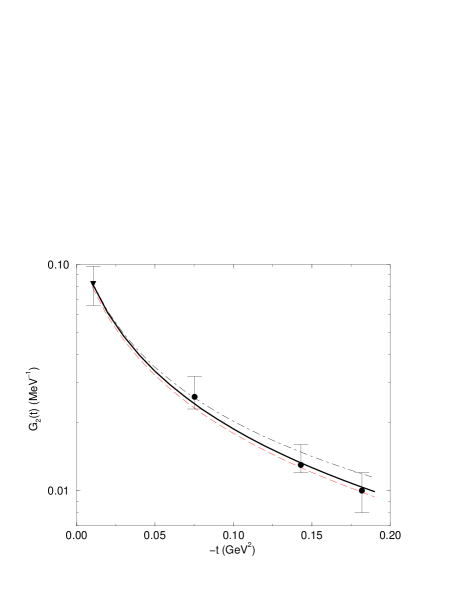
FIG. 1.: The pseudoscalar form factor for spacelike $t$. The dotted line is the pion pole prediction and the solid line includes the one-loop form of $\overline{G}_{2}$. The dashed-dotted line is from using the one-loop form for both $G_{1}$ and $\overline{G}_{2}$.

Finally, the scalar form factor cannot be directly measured, but is important in that its value at the Cheng-Dashen point may be tied to the pion-nucleon scattering data by dispersion analysis [28]. It is defined as

$\displaystyle\langle N(p_{2})|\hat{\sigma}(0)|N(p_{1})\rangle=F_{S}(t)\overline{u}(p_{2})u(p_{1})$

$$F_{S}(t) = -\frac{1+c}{f_{\pi}\Lambda}-\frac{3}{2f_{\pi}^{3}}\left(g_{A}\tilde{G}+\frac{m_{\pi}^{2}}{\Lambda}\right)\overline{J^{\pi\pi}}(t)$$ (24)

$${}-\frac{3G^{2}}{f_{\pi}^{3}}\Bigg{[}m_{N}\left(\overline{\Gamma^{N\pi}}(t)-2\overline{\Gamma^{N\pi}_{1}}(t)\right)$$

$$\qquad+\frac{1+c}{\Lambda}\left(\overline{J^{NN}}(t)+m_{\pi}^{2}\overline{\Gamma^{\pi N}}(t)\right)\Bigg{]}$$

The fact that we have kept $\sigma_{\pi N}$ to tree level in the Lagrangian shows up here as the leading piece in $F_{S}(t)$. Since we renormalize this quantity on-shell, no subtraction constants appear here. Other than this fact, we agree with GSS for $\Lambda\to\infty$. Note that, unlike in the vector form factors, the coefficients of the terms do not group exclusively into factors of $G/f_{\pi}$ showing different factors from just the naive $g_{\pi NN}$.

Defining $\sigma(t)=-m_{\pi}^{2}f_{\pi}F_{S}(t)$ as used by other authors with $\sigma(0)=\sigma_{\pi N}$, we can use eq. (24) to give a prediction for the scalar form factor at the Cheng-Dashen point $t=2m_{\pi}^{2}$ [3]. The value of the sigma term obtained from elastic $\pi N$ scattering (at $t=2m_{\pi}^{2}$) as compared to the value from the baryon mass spectrum (at $t=0$) is about $20$ MeV larger [32]. A numerical evaluation shows for $\sigma_{\pi N}=20$ MeV that the difference $\sigma(2m_{\pi}^{2})-\sigma(0)=5.3$ MeV and is not large enough to account for this discrepancy. This observation is similar to GSS.

VII One-Loop $\pi N$ Scattering

In order to calculate $\pi N$ scattering to one-loop, we only need the two-axial-vector correlator to one-loop since the vector and scalar form factors were evaluated in the previous section. Defining

$\displaystyle{\cal T}^{\pm}=A^{\pm}+\frac{1}{2}(\hbox to0.0pt{/\hss}k_{1}+\hbox to0.0pt{/\hss}k_{2})B^{\pm},$

and using the Mandelstam variables $s=(p_{1}+k_{1})^{2}$ and $t=(k_{1}-k_{2})^{2}$, the tree and one-loop result for the form factors can be written as

$$A^{+}_{S}=\frac{\sigma(t)}{f_{\pi}^{2}} \qquad A^{-}_{V}=-\frac{s-u}{8f_{\pi}^{2}m_{N}}F_{2}(t)$$

$$B^{-}_{V}=\frac{1}{2f_{\pi}^{2}}\left[F_{1}(t)+F_{2}(t)\right].$$

The rest of the tree result comes from the Born terms of $\langle N|T^{*}{\bf j}_{A}{\bf j}_{A}|N\rangle$ .

$$A^{+}_{AA,tree} = \frac{g_{A}\tilde{G}}{f_{\pi}^{2}}\qquad A^{-}_{AA,tree}=0$$

$$B^{+}_{AA,tree} = -\frac{G^{2}}{f_{\pi}^{2}}\left(\frac{1}{s-m_{N}^{2}}-\frac{1}{u-m_{N}^{2}}\right)$$

$$B^{-}_{AA,tree} = -\frac{g_{A}^{2}}{2f_{\pi}^{2}}-\frac{G^{2}}{f_{\pi}^{2}}\left(\frac{1}{s-m_{N}^{2}}+\frac{1}{u-m_{N}^{2}}\right)$$

with $\tilde{G}=2G-g_{A}m_{N}$. Its one-loop contribution is quoted in Appendix B.

Analyzing the divergence structure of the one-loop amplitude shows that it contains six independent subtraction constants for the total crossing symmetric amplitude

$$f_{\pi}^{4}A^{+}_{div.}=m_{N}t\;c_{1}+m_{N}^{3}\;c_{2}$$

$$f_{\pi}^{4}A^{-}_{div.} = m_{N}(s-u)\;c_{3}\qquad f_{\pi}^{4}B^{+}_{div.}=(s-u)\;c_{4}$$

$$f_{\pi}^{4}B^{-}_{div.}=t\;c_{5}+m_{N}^{2}\;c_{6}.$$

These six constants are in one-to-one correspondence with the six renormalized constants of GSS: $c^{r}_{1-4}$, $b^{r}_{2}$, and $b^{r}_{5}$. The five additional finite constants in [4] have no counterpart here. This is a direct consequence of our minimality assumption: only taking into account the divergent constants.

The constants may be fixed at subthreshold $s=u$, $t=0$ by fixing the following constants defined in [28, 33]

$$a^{+}_{00}=(-1.28\pm 0.24)/m_{\pi}\qquad b^{+}_{00}=(-3.54\pm 0.06)/m_{\pi}^{3}$$

$$a^{-}_{00}=(-8.83\pm 0.10)/m_{\pi}^{2}\qquad b^{-}_{00}=(10.36\pm 0.10)/m_{\pi}^{2}$$

$$a^{+}_{01}=(1.14\pm 0.02)/m_{\pi}^{3}\qquad b^{-}_{01}=(0.24\pm 0.01)/m_{\pi}^{4}.$$

Since we will be only looking at reactions in the forward direction ($t=0$) below, the coefficients of $t$, $a^{+}_{01}$ and $b^{-}_{01}$, will not be discussed further. Using the conventional model for the inclusion of the $\Delta(1232)$ [28] (we take $g_{\Delta}^{2}/4\pi=17.7$ GeV^-2 as in [34] and $Z=\frac{1}{2}$ as in the original Rarita-Schwinger paper for the non-pole $\Delta$ terms [35]), the contribution of the $\Delta$ included in the experimental subthreshold values is

$$a^{+\Delta}_{00}=-1.11/m_{\pi}\qquad b^{+\Delta}_{00}=-4.86/m_{\pi}^{3}$$

$$a^{-\Delta}_{00}=-11.34/m_{\pi}^{2}\qquad b^{-\Delta}_{00}=11.62/m_{\pi}^{2}.$$

One can see that these contributions are large and need to be taken into account for a proper fit. We have analytically checked that for any value of $Z$ and indeed even for the case where the non-pole terms are neglected the final result for the scattering lengths presented below is identical. The only difference is that part of the strength of the $\Delta$ contribution is shifted from subthreshold to threshold; the overall difference between the subthreshold and threshold remaining the same. Our choice $Z=1/2$ is merely for convenience since for this value the $\Delta$ contribution vanishes at threshold.

Moving to threshold, a prediction on the scattering lengths can be made to one-loop. Taking $g_{\pi NN}=G/f_{\pi}=13.3$, a reasonable result is found for $\sigma_{\pi N}=53$ MeV

$\displaystyle a^{+}_{\rm 1\,loop}\simeq 2.1\times 10^{-3}/m_{\pi}\qquad a^{-}_{\rm 1\,loop}\simeq 12\times 10^{-2}/m_{\pi}.$

The value for $a^{+}$ is close to the weighted average discussed in section V whereas $a^{-}$ is somewhat large. The results are very sensitive to the $\Delta$ contribution. Taking $\sigma_{\pi N}=45$ MeV gives $a^{+}=-8.7\times 10^{-3}/m_{\pi}$ without changing $a^{-}$. Taking $\sigma_{\pi N}=0$ and $G=g_{A}m_{N}$ give $(a^{+},a^{-})=(-4.8,10)\times 10^{-2}/m_{\pi}$ similar to [36]. A more recent calculation [25] finds $a^{+}=-10\times 10^{-3}/m_{\pi}$. This shows that the contribution of the $1/\Lambda$ terms to one-loop really makes a large difference.

Both scattering lengths come from large cancellations between the constants that were fixed at subthreshold and the loop contribution. This cancellation is needed due to the close proximity of the tree result to experiment. The large contribution from the $\Delta$ clouds the predictability, but our one-loop analysis seems to favor a value of $\sigma_{\pi N}$ close to the commonly accepted value of $45\pm 8$ MeV [32] and a small but positive $a^{+}$ scattering length. Both of these results are in contrast to [25] and rely on the non-zero value of $\sigma_{\pi N}$ and the Goldberger-Treiman discrepancy at tree level. The value for $a^{-}$ is about $20\%$ off from the experimental extrapolation from the Karlsruhe-Helsinki data.

The ability to fix $g_{A}$ and $g_{\pi NN}$ independently from experiment allows for a satisfactory starting point to the sensitive prediction of the $\pi N$ scattering lengths and can also lead to an estimation of $\sigma_{\pi N}$. The above analysis, however, showed an extreme sensitivity of the threshold results in $\pi N$ scattering and call for further study in the future.

VIII $\pi N\to\pi\pi N$ and the Pion-Nucleon Sigma Term

As a final estimate on the value of $\sigma_{\pi N}$, we turn to the process $\pi^{a}(k_{1})N(p_{1})\to\pi^{b}(k_{2})\pi^{c}(k_{3})N(p_{2})$. The scattering amplitude $i{\cal T}_{3\pi}$ fulfills an identity which can be derived by chiral reduction from the master formula approach [7] similar to what was done for $\pi N$ scattering. Defining the Mandelstam variables for a three body process [37]

$$s=(p_{1}+k_{1})^{2}\qquad s_{1}=(p_{2}+k_{3})^{2}\qquad s_{2}=(k_{2}+k_{3})^{2}$$

$$\qquad t_{1}=(p_{1}-p_{2})^{2}\qquad t_{2}=(k_{1}-k_{2})^{2},$$

the identity is

$\displaystyle i{\cal T}_{3\pi}=\left\{i{\cal T}_{\pi}+i{\cal T}_{A}+i{\cal T}_{SA}+i{\cal T}_{VA}\right\}+{\rm 2\ perms}+i{\cal T}_{AAA}$

$$i{\cal T}_{\pi}=\frac{i}{f_{\pi}^{2}}(t_{2}-m_{\pi}^{2})\delta^{ab}\langle N(p_{2})|\pi^{c}(0)|N(p_{1})\rangle$$

$$i{\cal T}_{A}=\frac{1}{2f_{\pi}^{3}}(k_{2}-k_{1})^{\mu}\delta^{ab}\langle N(p_{2})|{\bf j}^{c}_{A\mu}(0)|N(p_{1})\rangle$$

$$i{\cal T}_{SA}=-\frac{im_{\pi}^{2}}{f_{\pi}^{2}}k_{3}^{\mu}\delta^{ab}\int\!d^{4}xe^{-i(k_{1}-k_{2})\cdot x}$$

$$\qquad\qquad\times\langle N(p_{2})|T^{*}\hat{\sigma}(x){\bf j}_{A\mu}^{c}(0)|N(p_{1})\rangle$$

$$i{\cal T}_{VA}=\frac{1}{f_{\pi}^{3}}k_{1}^{\mu}k_{3}^{\nu}\epsilon^{abe}\int\!d^{4}x\;e^{-i(k_{1}-k_{2})\cdot x}$$

$$\qquad\qquad\times\langle N(p_{2})|T^{*}{\bf V}_{\mu}^{e}(x){\bf j}_{A\nu}^{c}(0)|N(p_{1})\rangle$$

$$i{\cal T}_{AAA}=-\frac{1}{f_{\pi}^{3}}k_{1}^{\mu}k_{2}^{\nu}k_{3}^{\lambda}\int\!d^{4}x_{1}d^{4}x_{2}\;e^{-ik_{1}\cdot x_{1}+ik_{2}\cdot x_{2}}$$

$$\qquad\qquad\times\langle N(p_{2})|T^{*}{\bf j}_{A\mu}^{a}(x_{1}){\bf j}_{A\nu}^{b}(x_{2}){\bf j}_{A\lambda}^{c}(0)|N(p_{1})\rangle$$

with “perms” meaning a permutation of $(k_{1},a;$ $-k_{2},b;$ $-k_{3},c)$. The structure of the chiral reduction formula immediately shows that the amplitude depends on $\sigma_{\pi N}$ (through the appearance of the scalar current $\hat{\sigma}$ in the ${\cal T}_{SA}$ term) allowing for an alternative way to fix its value.

At threshold, the amplitude can be decomposed as (see [38])

$\displaystyle i{\cal T}^{cba}=\frac{\vec{\sigma}\cdot\vec{k_{1}}}{2m_{N}}\left[{\cal D}_{1}(\tau^{b}\delta^{ac}+\tau^{c}\delta^{ab})+{\cal D}_{2}\tau^{a}\delta^{bc}\right].$

The tree contribution to the threshold amplitudes are

$$f_{\pi}^{3}{\cal D}_{1}=\frac{3}{2}\left(\frac{m_{N}+m_{\pi}}{m_{N}+2m_{\pi}}\right)\left[\;\frac{m_{N}+2m_{\pi}}{2m_{N}+m_{\pi}}\;G+2\overline{\Delta}_{\pi N}\right]$$

$${}-\frac{1}{4}(2m_{N}+m_{\pi})\left[g_{A}+\frac{3\overline{\Delta}_{\pi N}}{m_{N}+2m_{\pi}}\right]$$

$${}+\sigma_{\pi N}\left[g_{A}+\frac{m_{\pi}G}{(m_{N}+m_{\pi})(2m_{N}+m_{\pi})}\right]$$

$${}+\frac{1}{4}(2m_{N}+3m_{\pi})\Bigg{[}\frac{g_{A}}{4}-\frac{2m_{N}G}{(2m_{N}+m_{\pi})(m_{N}+m_{\pi})}$$

$$\qquad\qquad{}-\frac{3\overline{\Delta}_{\pi N}}{m_{N}+2m_{\pi}}\Bigg{]}$$

$${}+\frac{g_{A}^{2}}{2}(G-2\overline{\Delta}_{\pi N})-\frac{g_{A}^{3}m_{\pi}}{2}$$

$${}-\frac{G}{(m_{N}+m_{\pi})(2m_{N}+m_{\pi})}\Bigg{(}\frac{g_{A}^{2}m_{\pi}^{2}}{2}-g_{A}m_{\pi}\tilde{G}$$

$$\qquad\qquad{}+\frac{2(m_{N}+2m_{\pi})G^{2}}{2m_{N}+m_{\pi}}\Bigg{)}$$

$$f_{\pi}^{3}{\cal D}_{2}=-\frac{3}{2}\left[\;\frac{m_{N}+2m_{\pi}}{2m_{N}+m_{\pi}}\;G+2\overline{\Delta}_{\pi N}\right]$$

$${}+\frac{m_{\pi}}{2}\left[g_{A}+\frac{3\overline{\Delta}_{\pi N}}{m_{N}+2m_{\pi}}\right]$$

$${}+\sigma_{\pi N}\left[g_{A}-\frac{G}{2}\frac{4m_{N}+5m_{\pi}}{2m_{N}^{2}+2m_{N}m_{\pi}-m_{\pi}^{2}}\right]$$

$${}-\frac{1}{2}(2m_{N}+3m_{\pi})\Bigg{[}\frac{g_{A}}{4}-\frac{2m_{N}G}{(2m_{N}+m_{\pi})(m_{N}+m_{\pi})}$$

$$\qquad\qquad{}-\frac{3\overline{\Delta}_{\pi N}}{m_{N}+2m_{\pi}}\Bigg{]}$$

$${}+\frac{g_{A}^{2}}{2}(G-2\overline{\Delta}_{\pi N})+g_{A}^{3}(m_{N}+m_{\pi})$$

$${}-\frac{g_{A}G\tilde{G}}{2}\frac{4m_{N}+5m_{\pi}}{2m_{N}^{2}+2m_{N}m_{\pi}-m_{\pi}^{2}}$$

$${}-\frac{2G}{(2m_{N}+m_{\pi})(m_{N}+m_{\pi})}\Bigg{(}\frac{g_{A}^{2}}{4}(6m_{N}^{2}+9m_{N}m_{\pi}+m_{\pi}^{2})$$

$$\qquad{}-\frac{G^{2}}{2}\frac{4m_{N}+5m_{\pi}}{2m_{N}+m_{\pi}}\Bigg{)}.$$

The brackets section off, in order, the contribution of the first four terms in the chiral reduction formula. The contribution from ${\cal T}_{AAA}$ is given by the remaining terms. This calculation is in agreement with [39] if we take $\Lambda\to\infty$. Note the explicit dependence on $\sigma_{\pi N}$ in the threshold amplitudes. Taking $\overline{\Delta}_{\pi N}=-54$ MeV for the proper value of $g_{\pi NN}$, $\sigma_{\pi N}=53$ MeV as in the previous section, and defining $D_{i}={\cal D}_{i}/2m_{N}$, we find

$\displaystyle D_{1}=2.78\mbox{\ fm}^{3}\qquad D_{2}=-6.59\mbox{\ fm}^{3}$

whereas experimentally [40]

$\displaystyle D_{1}^{\rm exp}=1.82\pm 0.09\mbox{\ fm}^{3}\qquad D_{2}^{\rm exp}=-7.30\pm 0.24\mbox{\ fm}^{3}.$

Although both $D_{i}$’s depend on $\sigma_{\pi N}$, only $D_{1}$ is sensitive to it, decreasing to $D_{1}=2.5$ fm³ for $\sigma_{\pi N}=14$ MeV. Therefore experiment seems to favor a smaller $\sigma_{\pi N}$.

The large $30\%$ discrepancy in $D_{1}$ reflects on the difficulty in extracting the threshold parameters. A different fit in the literature [41] gives $(D_{1},D_{2})=(2.26,-9.05)$ fm³. Furthermore, large corrections occur in ChPT from higher order terms bringing the convergence of this parameter into question. The one-loop corrections to the $D_{i}$’s will be presented elsewhere.

IX Conclusions

We have introduced a minimal model for $\pi N$ dynamics that embodies uniquely at tree level the main features of broken chiral symmetry with on-shell pions and nucleons to all orders. Using this on-shell expansion and a BPHZ subtraction scheme, we have shown how the chiral reduction formula be enforced with a minimal number of parameters. All of our results are consistent with data.

With this simple model we have analyzed the axial Ward identity derived in section IV as well as a Ward identity for $\pi N$ scattering originally derived by Weinberg and a new chiral reduction formula for $\pi N\to\pi\pi N$. We have presented a one-loop calculation of the nucleon form factors and $\pi N$ scattering and shown their equivalence to ChPT in the $\Lambda\to\infty$ limit.

For finite $\Lambda$, this model has the additional feature of allowing room for $g_{A}$, $m_{N}$, $g_{\pi NN}$, and $\sigma_{\pi N}$ to be fixed to their phenomenological values — all at tree level in a $1/f_{\pi}$ loop expansion. In particular, an estimate can be made on the value of $\sigma_{\pi N}$ from various processes. Terms proportional to $\sigma_{\pi N}$ are certainly important in the scalar form factor $F_{S}(t)$, the $\pi N$ scattering length $a^{+}$, and the threshold parameter $D_{1}$ from the $\pi N\to\pi\pi N$ process.

The only hindrance in nailing down a more stringent prediction on $\sigma_{\pi N}$ comes from determining the contribution of nucleonic resonances such as the $\Delta(1232)$ at the point where the divergent constants are fixed. An ideal situation would be to find an amplitude with the divergences constrained by current conservation and yet still dependent on $\sigma_{\pi N}$ for an unambiguous determination of the pion-nucleon sigma term. Photo-production $\gamma N\to\pi N$ may be such a case.

On-shell renormalization along with the approach of using a minimal amount of parameters dictated purely by the divergences increases the predictability of the model due to fewer constraints needed to fix the constants. In particular, there are no constants in $F_{2}(t)$ or $F_{S}(t)$ as opposed to one each in ChPT and there are six constants in $\pi N$ scattering as opposed to eleven in ChPT.

The analysis of $\pi N$ scattering shows that all six of the subtraction constants in the amplitude can be fixed at subthreshold. Including the $\Delta(1232)$ contribution, the scattering lengths can be predicted with reasonable accuracy. The value of $\sigma_{\pi N}$ as constrained from $\pi N$ scattering goes from being on the lower side of the canonically accepted value of $45\pm 8$ MeV [32] at tree level to within the predicted accuracy at one-loop, showing an improvement upon adding loop corrections as expected.

We have kept a relativistic formulation in order to maintain relativistic unitarity. Indeed, many HBChPT calculations, although formulated with a heavy baryon Lagrangian, tend to start with the relativistic Feynman rules and only after evaluation of the amplitude take the non-relativistic limit. This is not only more natural but keeps from missing terms as could happen from the non-relativistic formulation.

The convergence of a relativistic calculation crucially depends on the appearance of the constant terms $m_{N}^{2}/(4\pi f_{\pi})^{2}$. Although such terms do appear, in all the cases considered here they are always accompanied by a divergent subtraction constant. A mere redefinition of this arbitrary constant removes such terms from the expansion and rectifies the convergence. Whether this is a general feature of the loop expansion employed here merits further investigation.

A

The Feynman rules from ${\cal L}_{1+2}$ needed in this paper are ones with external current lines and internal (loop) pion lines. We take the transformation ${\bf\Psi}_{i}\to\xi_{i}\psi_{i}$ ($i=R,L$) with $U=\xi_{R}\xi_{L}^{\dagger}$ and choose $\xi_{R}=\xi_{L}^{\dagger}$. The rules for the $\psi$ nucleon fields are

All loop processes in this paper can be expressed in terms of the following general Feynman parameter integrals. Here $dk$ is shorthand for $d^{4}k/(2\pi)^{4}$ properly regularized and $[p]_{a}=(k+p)^{2}-m_{a}^{2}$. For two propagators, the integrals are

$$-i\int\!\!dk\frac{(1;\;k_{\mu};\;k_{\mu}k_{\nu})}{[-p]_{a}[0]_{b}}\equiv\left(J;\;p_{\mu}J_{1};\;p_{\mu}p_{\nu}J_{21}+g_{\mu\nu}J_{22}\right)$$

with $J_{i}=J^{ab}_{i}(p^{2})$,

$$\left(\overline{J};\;\overline{J_{1}};\;\overline{J_{21}}\right)=-\int_{0}^{1}\!\frac{dx}{(4\pi)^{2}}\;\ln\frac{h_{J}(p^{2})}{h_{J}(p^{2}_{0})}\;(1;\;x;\;x^{2})$$

$$\overline{\overline{J_{22}}}=-\!\int_{0}^{1}\!\!\!\frac{dx}{2(4\pi)^{2}}\bigg{[}h_{J}(p^{2})\ln\frac{h_{J}(p^{2})}{h_{J}(p^{2}_{0})}+x(1-x)(p^{2}-p^{2}_{0})\bigg{]}$$

$\displaystyle h_{J}(s)=m_{a}^{2}x+m_{b}^{2}(1-x)-s\,x(1-x),$

and $p^{2}_{0}$ is the subtraction point. The number of bars above a function denote how many terms of its Taylor series are subtracted at the chosen point. Note that $J^{aa}=2J^{aa}_{1}$.

For three propagators, since there are only two particles which play a role in the loops (nucleon and pion), two of the propagators will certainly have the same mass.

$$-i\int\!\!dk\frac{(1;\;k_{\mu};\;k_{\mu}k_{\nu};k_{\mu}k_{\nu}k_{\rho})}{[0]_{a}[-p]_{b}[-q]_{b}}\equiv\Bigg{(}\Gamma;\;Q_{\mu}\Gamma_{1}+P_{\mu}\Gamma_{2};\;$$

$$\qquad\qquad\qquad g_{\mu\nu}\Gamma_{3}+Q_{\mu}Q_{\nu}\Gamma_{4}+Q_{(\mu}P_{\nu)}\Gamma_{5}+P_{\mu}P_{\nu}\Gamma_{6}\Bigg{)}$$

with $(Q,P)=(p+q,p-q)$, $\Gamma_{i}=\Gamma^{ab}(p^{2},q^{2},P^{2})$. The finite integrals are

$$\Gamma_{i}=-\frac{1}{(4\pi)^{2}}\int_{0}^{1}\!dx\,dy\;y\;\frac{\alpha_{i}}{h_{\Gamma}}$$

with

$$\alpha = 1\qquad\alpha_{1}=\frac{y}{2}\qquad\alpha_{2}=\frac{y}{2}(2x-1)$$

$$\alpha_{4} = \frac{y^{2}}{4}\qquad\alpha_{5}=\frac{y^{2}}{4}(2x-1)\qquad\alpha_{6}=\frac{y^{2}}{4}(2x-1)^{2}$$

and

$$h_{\Gamma} = m_{a}^{2}(1-y)+m_{b}^{2}y-p^{2}xy(1-y)$$

$${}-q^{2}(1-x)y(1-y)-P^{2}x(1-x)y^{2}.$$

The divergent function can be subtracted to give

$$\overline{\Gamma}_{3}=-\frac{1}{2(4\pi)^{2}}\int_{0}^{1}\!dx\,dy\;y\;\ln\frac{h_{\Gamma}}{h_{\Gamma,0}}$$

with $\Gamma_{i}(m_{N}^{2},m_{N}^{2},P^{2})=\Gamma_{i}(P^{2})$ and $\Gamma_{i}(s,m_{N}^{2},P^{2})=\Gamma_{i}(s,P^{2})$ shorthand notation used in this paper.

Finally we need the following functions for four propagators

$$-i\int\!dk\,\frac{(1;\;k_{\mu};\;k_{\mu}k_{\nu})}{[0]_{\pi}[-p]_{N}[-q]_{N}[-r]_{N}}\equiv\left({\cal G};\;p_{\mu}{\cal G}_{1}+q_{\mu}{\cal G}_{2}+r_{\mu}{\cal G}_{3}\right)$$

with ${\cal G}_{i}={\cal G}^{\pi N}_{i}(p,q,r)$. All four integrals are finite

$\displaystyle{\cal G}_{i}=\frac{1}{(4\pi)^{2}}\int_{0}^{1}\!dx\,dy\,dz\,y^{2}z\frac{\beta_{i}}{h_{\cal G}^{2}}$

with

$\displaystyle\beta=1\qquad\beta_{1}=xyz\qquad\beta_{2}=(1-x)yz\qquad\beta_{3}=(1-z)y$

For this paper only the form ${\cal G}^{\pi N}_{i}(p_{1}+q_{1},p_{1},p_{2})$ with $p_{1}^{2}=p_{2}^{2}=m_{N}^{2}$, $p_{1}+q_{1}=p_{2}+q_{2}$ and $q_{1}^{2}=q_{2}^{2}=m_{\pi}^{2}$ was used, for which ${\cal G}^{\pi N}_{1}={\cal G}^{\pi N}_{2}$ and

$$h_{G} = m_{\pi}^{2}(1-y)+m_{N}^{2}y^{2}-(s-m_{N}^{2})y(1-y)(1-z)$$

$${}-m_{\pi}^{2}y^{2}z(1-z)-tx(1-x)(yz)^{2}$$

with $s=(p_{1}+q_{1})^{2}$ and $t=(p_{1}-p_{2})^{2}$.

B

The one-loop form for the two axial-vector correlator $\langle N|T^{*}{\bf j}_{A}{\bf j}_{A}|N\rangle$ is quoted below. This is needed for $\pi N$ scattering. Using the notation $\overline{\Delta}_{\pi N}=g_{A}m_{N}-G$ we find:

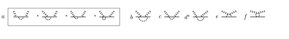
FIG. 2.: One-loop diagrams for $\pi N$ scattering. The graphs with a star also have a mirror image diagram which must be taken into account and all graphs except for those in the last line require the addition of a crossed diagram.

Writing $A^{\pm}=A^{\pm}(s,t,u)\pm A^{\pm}(u,t,s)$ and $B^{\pm}=B^{\pm}(s,t,u)\mp B^{\pm}(u,t,s)$ to take into account the crossed diagrams, we only quote the contribution from the direct diagrams shown in fig. 2. The self energy and form factor contributions of fig. 2a can be written succinctly with the use of the axial-vector nucleon form factors with one off-shell nucleon leg [15]. With the understanding of only taking this to order $1/f_{\pi}^{4}$, it can be written as

$$A^{\pm}_{\ref{piN}a}(s,t,u) = \frac{1}{4f_{\pi}^{2}}\frac{\sqrt{s}-m_{N}}{\sqrt{s}}f_{s.e.}(\sqrt{s})\left[g(\sqrt{s},m_{N},m_{\pi}^{2})\right]^{2}+(\sqrt{s}\to-\sqrt{s})$$

$$B^{\pm}_{\ref{piN}a}(s,t,u) = -\frac{1}{4f_{\pi}^{2}}\frac{1}{\sqrt{s}}f_{s.e.}(\sqrt{s})\left[g(\sqrt{s},m_{N},m_{\pi}^{2})\right]^{2}+(\sqrt{s}\to-\sqrt{s})$$

with $g=(\sqrt{s}+m_{N})g_{1}+m_{\pi}^{2}\overline{g}_{2}-(s-m_{N}^{2})g_{3}$,

$$f_{s.e.}(\sqrt{s}) = \frac{1}{\sqrt{s}-m_{N}}+\frac{3}{4f_{\pi}^{2}}\frac{(g_{A}\sqrt{s}+\tilde{G})^{2}}{(\sqrt{s}-m_{N})^{2}}\left[m_{N}\overline{J^{\pi N}}(s)-\sqrt{s}\,\overline{J^{\pi N}_{1}}(s)\right]-\frac{3m_{N}^{2}}{2f_{\pi}^{2}}\frac{(g_{A}\sqrt{s}+\tilde{G})^{2}}{\sqrt{s}-m_{N}}\left[J^{\pi N}{}^{\prime}(m_{N}^{2})-J^{\pi N}_{1}{}^{\prime}(m_{N}^{2})\right]$$

$$g_{1}(\sqrt{s},m_{N},t)=g_{A}+\frac{g_{A}^{2}-4}{4f_{\pi}^{2}}\left(g_{A}\sqrt{s}+\tilde{G}\right)\left[m_{N}\overline{J^{\pi N}}(s)-\sqrt{s}\,\overline{J^{\pi N}_{1}}(s)\right]$$

$$\qquad{}+\frac{g_{A}G}{2f_{\pi}^{2}}\left(g_{A}\sqrt{s}+\tilde{G}\right)\bigg{[}-2\overline{\Gamma^{\pi N}_{3}}(s,t)+\overline{J^{NN}}(t)+m_{\pi}^{2}\Gamma^{\pi N}(s,t)-(s-m_{N}^{2})\Gamma^{\pi N}_{1}(s,t)-(\sqrt{s}-m_{N})^{2}\Gamma^{\pi N}_{2}(s,t)\bigg{]}$$

$$\overline{g}_{2}(\sqrt{s},m_{N},t)=-\frac{2}{\Lambda}+\frac{g_{A}-2(1+c)}{2f_{\pi}^{2}\Lambda}\left(g_{A}\sqrt{s}+\tilde{G}\right)\left[m_{N}\overline{J^{\pi N}}(s)-\sqrt{s}\overline{J^{\pi N}_{1}}(s)\right]$$

$$\qquad{}-\frac{G}{f_{\pi}^{2}\Lambda}\left(g_{A}\sqrt{s}+\tilde{G}\right)\left[\overline{J^{NN}}(t)+m_{\pi}^{2}\Gamma^{\pi N}(s,t)-(\sqrt{s}-m_{N})^{2}\Gamma^{\pi N}_{1}(s,t)-(s-m_{N}^{2})\Gamma^{\pi N}_{2}(s,t)\right]$$

$$\qquad{}-\frac{g_{A}G}{2f_{\pi}^{2}}\left(g_{A}\sqrt{s}+\tilde{G}\right)\left[(\sqrt{s}-m_{N})\left(2\Gamma^{\pi N}_{5}(s,t)-\Gamma^{\pi N}_{1}(s,t)-\Gamma^{\pi N}_{2}(s,t)\right)+2(\sqrt{s}+m_{N})\Gamma^{\pi N}_{6}(s,t)\right]$$

$$\qquad{}+\frac{4G}{f_{\pi}^{2}}\left(g_{A}\sqrt{s}+\tilde{G}\right)\left[\frac{G}{m_{\pi}^{2}-t}\underline{\underline{J^{NN}}}(t)+\frac{1}{\Lambda}\underline{J^{NN}}(t)\right]$$

$$g_{3}(\sqrt{s},m_{N},t)=\frac{g_{A}G}{2f_{\pi}^{2}}\left(g_{A}\sqrt{s}+\tilde{G}\right)\Bigg{[}2(\sqrt{s}-m_{N})\Gamma^{\pi N}_{4}(s,t)+2(\sqrt{s}+m_{N})\Gamma^{\pi N}_{5}(s,t)$$

$$\qquad\qquad\qquad\qquad{}+(\sqrt{s}-m_{N})\Gamma^{\pi N}_{1}(s,t)+(\sqrt{s}-m_{N})\Gamma^{\pi N}_{2}(s,t)\Bigg{]},$$

and $\tilde{G}=2G-g_{A}m_{N}$. It can be checked by the Ward identity in eq. (17) that $g(m_{N},m_{N},m_{\pi}^{2})\equiv 2f_{\pi}g_{\pi NN}$ exactly to one loop therefore showing a simple way in which the on-shell values are maintained. The other graphs in fig. 2 give

$$f_{\pi}^{4}A^{+}_{\ref{piN}b}(s,t,u) = \frac{3}{16}g_{A}^{2}m_{N}\left[g_{A}^{2}(s-m_{N}^{2})+4\tilde{G}^{2}\right]\overline{J^{\pi N}}(s)$$

$${}+\frac{3}{16}g_{A}^{2}\left[2g_{A}s(\tilde{G}-2\overline{\Delta}_{\pi N})+m_{N}\left(g_{A}^{2}s+(\tilde{G}-2\overline{\Delta}_{\pi N})^{2}\right)\right]\overline{J^{\pi N}_{1}}(s)$$

$${}+3g_{A}\tilde{G}G^{2}\left[-\overline{J^{NN}}(m_{\pi}^{2})-m_{\pi}^{2}\Gamma^{\pi N}(s)+(s+3m_{N}^{2})\Gamma^{\pi N}_{1}(s)+(s-m_{N}^{2})\Gamma^{\pi N}_{2}(s)\right]$$

$${}+3g_{A}^{2}m_{N}G^{2}(s-m_{N}^{2})\Gamma^{\pi N}_{1}(s)+\frac{3}{2}g_{A}^{2}G^{2}m_{N}(s-u)\Gamma^{\pi N}_{4}(t)-6m_{N}G^{4}\Gamma^{\pi N}_{1}(t)$$

$${}+\frac{3}{2}g_{A}\tilde{G}G^{2}\left[\overline{J^{NN}}(t)+m_{\pi}^{2}\Gamma^{\pi N}(t)\right]+3m_{N}G^{4}(s-m_{N}^{2})\left[2{\cal G}^{\pi N}_{1}+{\cal G}^{\pi N}_{3}\right]$$

$$f_{\pi}^{4}B^{+}_{\ref{piN}b}(s,t,u) = \frac{3}{8}g_{A}^{3}m_{N}(\tilde{G}-2\overline{\Delta}_{\pi N})\overline{J^{\pi N}}(s)+\frac{3}{16}g_{A}^{2}\left(g_{A}^{2}s+(\tilde{G}-2\overline{\Delta}_{\pi N})^{2}\right)\overline{J^{\pi N}_{1}}(s)$$

$${}+\frac{3}{2}g_{A}^{2}G^{2}\left[-\overline{J^{NN}}(m_{\pi}^{2})-m_{\pi}^{2}\Gamma^{\pi N}(s)+(s-m_{N}^{2})\left(\Gamma^{\pi N}_{1}(s)+\Gamma^{\pi N}_{2}(s)\right)\right]$$

$${}+\frac{3}{4}g_{A}^{2}G^{2}\left[2\overline{\Gamma^{\pi N}_{3}}(t)-\overline{J^{NN}}(t)-m_{\pi}^{2}\Gamma^{\pi N}(t)\right]+6g_{A}m_{N}\tilde{G}G^{2}\Gamma^{\pi N}_{1}(s)$$

$${}+3G^{4}\left[(s-m_{N}^{2}){\cal G}^{\pi N}_{3}-m_{\pi}^{2}{\cal G}^{\pi N}-\Gamma^{NN}(m_{\pi}^{2},m_{\pi}^{2},t)\right]$$

$$A^{-}_{\ref{piN}b}(s,t,u) = -\frac{1}{3}A^{+}_{\ref{piN}b}(s,t,u)\qquad\qquad\qquad B^{-}_{\ref{piN}b}(s,t,u)=-\frac{1}{3}B^{+}_{\ref{piN}b}(s,t,u)$$

$$f_{\pi}^{4}A^{+}_{\ref{piN}c}(s,t,u) = \frac{1}{2}m_{N}\left[(s-m_{N}^{2}+2\sigma_{\pi N}^{2})\overline{J^{\pi N}}(s)-(s-m_{N}^{2}-2\sigma_{\pi N}^{2})\overline{J^{\pi N}_{1}}(s)\right]$$

$$f_{\pi}^{4}A^{-}_{\ref{piN}c}(s,t,u) = \frac{1}{4}(s-m_{N}^{2})\left[m_{N}\overline{J^{\pi N}}(s)-(m_{N}-4\sigma_{\pi N})\overline{J^{\pi N}_{1}}(s)\right]$$

$$f_{\pi}^{4}B^{+}_{\ref{piN}c}(s,t,u) = -\frac{1}{2}\left[2m_{N}^{2}\overline{J^{\pi N}}(s)-(s+m_{N}^{2}+2\sigma_{\pi N}^{2})\overline{J^{\pi N}_{1}}(s)\right]$$

$$f_{\pi}^{4}B^{-}_{\ref{piN}c}(s,t,u) = -\frac{1}{4}\left[2m_{N}(m_{N}-2\sigma_{\pi N})\overline{J^{\pi N}}(s)-(s+m_{N}^{2}-4m_{N}\sigma_{\pi N})\overline{J^{\pi N}_{1}}(s)\right]$$

$$f_{\pi}^{4}A^{+}_{\ref{piN}d}(s,t,u) = -\frac{1}{2}g_{A}m_{N}\left(g_{A}(s-m_{N}^{2})-2\sigma_{\pi N}\tilde{G}\right)\overline{J^{\pi N}}(s)$$

$${}-\frac{1}{2}g_{A}\left((g_{A}m_{N}-4\overline{\Delta}_{\pi N})(s-m_{N}^{2})-g_{A}\sigma_{\pi N}(s+m_{N}^{2})+4m_{N}\overline{\Delta}_{\pi N}\sigma_{\pi N}\right)\overline{J^{\pi N}_{1}}(s)$$

$${}+2\sigma_{\pi N}G^{2}(s-m_{N}^{2})\Gamma^{\pi N}_{2}(s)-2\sigma_{\pi N}G^{2}\left(\overline{J^{NN}}(m_{\pi}^{2})+m_{\pi}^{2}\Gamma^{\pi N}(s)\right)$$

$$f_{\pi}^{4}B^{+}_{\ref{piN}d}(s,t,u) = \frac{1}{2}g_{A}m_{N}\left(g_{A}\sigma_{\pi N}+4\overline{\Delta}_{\pi N}\right)\overline{J^{\pi N}}(s)$$

$${}-\frac{1}{2}g_{A}\left(g_{A}(s-m_{N}^{2}-m_{N}\sigma_{\pi N})+2\overline{\Delta}_{\pi N}(2m_{N}+\sigma_{\pi N})\right)\overline{J^{\pi N}_{1}}(s)$$

$${}+2G^{2}\left(\overline{J^{NN}}(m_{\pi}^{2})+m_{\pi}^{2}\Gamma^{\pi N}(s)\right)$$

$${}-2G^{2}(s-m_{N}^{2})\left(\Gamma^{\pi N}_{1}(s)+\Gamma^{\pi N}_{2}(s)\right)+4m_{N}\sigma_{\pi N}G^{2}\Gamma^{\pi N}_{1}(s)$$

$$A^{-}_{\ref{piN}d}(s,t,u) = 0\qquad\qquad\qquad B^{-}_{\ref{piN}d}(s,t,u)=0$$

$$f_{\pi}^{4}A^{+}_{\ref{piN}e}(s,t,u) = (t-2m_{\pi}^{2})\left[g_{A}\tilde{G}\overline{J^{\pi\pi}}(t)+2m_{N}G^{2}\left(\Gamma^{\pi N}(t)-2\Gamma^{\pi N}_{1}(t)\right)\right]$$

$$f_{\pi}^{4}A^{+}_{\ref{piN}f}(s,t,u) = \sigma_{\pi N}(t-2m_{\pi}^{2})\overline{J^{\pi\pi}}(t)$$

In the $\Lambda\to\infty$ limit we reproduce all the finite parts of GSS. This shows that calculation of the $\pi N$ scattering amplitude using the Ward identity with external fields is equivalent to a calculation with the pion vertices from the Lagrangian without mention of external fields or the Ward identity. Whether this holds for $\pi N\to\pi\pi N$ will be discussed elsewhere.

The relation between the two calculations can be made more transparent by use of diagrams. The vector and scalar form factor contribution to the $\pi N$ Ward identity, along with the contact interactions from $\langle N|T^{*}{\bf j}_{A}{\bf j}_{A}|N\rangle$, are equivalent to the the graphs from the pion calculation which contain two external pions meeting at one point. Diagramatically this is just:

with the left-hand side containing the proper coefficient given by the Ward identity. The other possible graphs from the pion calculation are in one-to-one correspondence with the graphs of the same topology from the two axial-vector correlator.

REFERENCES

[1]
S.L. Adler, Phys. Rev. B 139 (1965) 1638; S. Weinberg,
Phys. Rev. Lett. 17 (1966) 616.
[2]
R.F. Dashen, Phys. Rev. 133(1969)1245; R. Dashen and M. Weinstein,
Phys. Rev. 133 (1969) 1291; H. Pagels, Phys. Rep. 16 (1975) 219;
J. Gasser and H. Leutwyler, Ann. Phys. 158 (1984) 142.
[3]
T.P. Cheng and R.F. Dashen, Phys. Rev. Lett. 26 (1971) 594.
[4]
J. Gasser, M.E. Sainio, and A. Švarc, Nucl. Phys. B 307 (1988)
779, and references therein.
[5]
S. Weinberg, “Lectures on Elementary Particles and Quantum Field
Theory,” Brandeis Summer Institute 1970, S. Deser, M. Grisaru, and
H. Pendleton, MIT Press, 1970.
[6]
Y. Tomozawa, Nuovo Cim. (Ser. X) 46A (1966) 707; S. Weinberg,
Phys. Rev. Lett. 17 (1966) 616; 18 (1967) 188, 507.
[7]
H. Yamagishi and I. Zahed, Phys. Rev. D53 (1996) 2288;
Ann. Phys. 247 (96) 292.
[8]
J.V. Steele, H. Yamagishi, and I. Zahed, Nucl. Phys. A615 (1997) 305.
[9]
I. Zahed and G.E. Brown, Phys. Rep. 142 (1986) 1; G. Holzwarth and
B. Schwesinger, Rep. Prog. Phys. 49 (1986) 825; Chiral Solitons,
ed. Keh-Fei Liu, World Scientific, 1987; Skyrmions and
Anomalies, ed. M. Jezabek and M. Praszalowicz, World Scientific, 1987.
[10]
H. Yamagishi and I. Zahed, Mod. Phys. Lett. A7 (1992) 1105,
and references therein.
[11]
H. Yamagishi and I. Zahed, ‘Chiral Solitons : a Difficulty’, SUNY-NTG-94-7,
unpublished.
[12]
C.G. Callan, S. Coleman, J. Wess, and B. Zumino, Phys. Rev. 177 (1969) 2247.
[13]
J.V. Steele, H. Yamagishi, and I. Zahed, hep-ph/9512233.
[14]
K. Nishijima, Nuov. Cim. (Ser. X) 11 (1959) 698;
F. Gursey, Nuov. Cim. (Ser. X) 16 (1960) 230.
[15]
J.V. Steele, H. Yamagishi, and I. Zahed, in preparation.
[16]
J. Stern, H. Sazdjian and N.H. Fuchs, Phys. Rev. D 47 (1993) 3814
[17]
V. Bernard, N. Kaiser and U.-G. Meissner, Phys. Lett. B309 (1993) 421.
[18]
E. Jenkins and A.V. Manohar, Phys. Lett. B 255 (1991) 558.
[19]
V. Bernard, N. Kaiser, J. Kambor, and U.-G. Meissner, Nucl. Phys. B 388
(1992) 315.
[20]
G. Ecker, Phys. Lett. B336 (1994) 508;
M. Mojzis, hep-ph/9704415, and references therein.
[23]
D. Chatellard, et al., Phys. Rev. Lett. 74 (1995) 4157.
[24]
R. Machleidt, ‘The meson Theory of Nuclear Forces and Nuclear Structure’,
in Advances in Nuclear Physics, Vol. 19, Eds. J.W. Negele and E. Vogt,
Plenum (1989), and references therein.
[25]
V. Bernard, N. Kaiser, and U.-G. Meissner, Nucl. Phys. A 615 (1997) 483.
[26]
J. Bernabéu, Nucl. Phys. A 374 (1982) 593c.
[27]
G. Bardin, et al., Phys. Lett. B 104 (1981) 320.
[28]
G. Höhler, In Landolt-Börnstein, Vol. 9 b2, ed. H. Schopper
(Springer, Berlin, 1983).
[29]
T. Kitigaki, et al., Phys. Rev. D 28 (1983) 436.
[30]
S. Choi, et al., Phys. Rev. Lett. 71 (1993) 3927.
[31]
S. Adler and Y. Dothan, Phys. Rev. 151 (1966) 1267; L. Wolfenstein,
in: High-Energy Physics and Nuclear Structure, ed. S. Devons, Plenum,
New York, 1970.
[32]
J. Gasser, H. Leutwyler, and M.E. Sainio, Phys. Lett. B 253 (1991) 260.
[33]
M.M. Nagels, et al., Nucl. Phys. B 147 (1979) 189.
[34]
M. Kacir and I. Zahed, Phys. Rev. D54 (1996) 5536.
[35]
W. Rarita and J. Schwinger, Phys. Rev. 60 (1941) 61.
[36]
J. Gasser, Nucl. Phys. B279 (1987) 65.
[37]
H.C. Eggers, R. Tabti, C. Gale, and K. Haglin, Phys.Rev. D 53 (1996) 4822.
[38]
V. Bernard, N. Kaiser, and U.-G. Meissner, Nucl.Phys. B 457 (1995) 147.
[39]
J. Beringer, Newslett. 7 (1992) 33.
[40]
G. Kernel, et al., Z. Phys. C48 (1990) 201; M. Sevior, et
al., Phys. Rev. Lett. 66 (1991) 2569; J. Lowe, et al.,
Phys. Rev. C44 (1991) 956.
[41]
V. Bernard, N. Kaiser, and U.-G. Meissner, Int. J. Mod. Phys. E4
(1995) 193.