The Solar Neutrino Problem in the Presence of
Flavor Changing Neutrino Interactions

Abstract

We study the effects of flavor changing neutrino interactions on the resonant conversion of solar neutrinos. In particular, we describe how the regions in the $\Delta m^{2}-\sin^{2}2\theta$ plane that are consistent with the four solar neutrino experiments are modified for different strengths of New Physics neutrino interactions.

1 Introduction

Neutrino oscillations [1, 2, 3, 4] are considered to be the most likely solution to the longstanding Solar Neutrino (SN) Problem [5, 6, 7]. The standard solution asserts that neutrinos have non-vanishing masses and that there is mixing. Many extensions of the Standard Model (SM), such as Left-Right Symmetric Models (LRSMs) [8] and Supersymmetric Models without $R$-parity [9], predict not only neutrino masses but also New Physics (NP) neutrino interactions that are not present in the SM.

The effects of NP on neutrino oscillations have been studied previously in the literature [10, 11, 12, 13, 14]. In [10] the effects of flavor changing neutrino interactions on the Mikheyev-Smirnov-Wolfenstein (MSW) effect [1] were considered and it was demonstrated that, even in the absence of neutrino mixing in vacuum, neutrino oscillations in matter can be enhanced by flavor changing neutral currents (FCNCs). In [11] it was shown that additional non-universal flavor diagonal neutral currents (FDNCs) may allow for resonantly enhanced neutrino transitions even if neutrinos have vanishing masses. Both scenarios as well as the case of massive neutrinos with off-diagonal and new diagonal currents were investigated thoroughly in Ref. [12]. This analysis also determined the regions in parameter space that gave consistency with the standard solar model (SSM) and the then available solar neutrino data from the Homestake [15] and Kamiokande [16] experiments. The implications on the allowed regions due to the more recent data from the two gallium detectors, GALLEX [17] and SAGE [18], were discussed in [13] for massive neutrinos and FCNCs (but no FDNCs). More recently also the solution to the SN Problem with both FCNCs and FDNCs but with massless neutrinos was re-analyzed [14], this time including the data from all four SN experiment and the latest improvements to the SSM [19].

In this work we reconsider the combination of neutrino masses and mixing with new flavor changing neutrino interactions (but without significant non-universal FDNCs). We update the previous analyses of this case by taking into account the most recent data from all four SN experiments and by using the latest improvements to the SSM. We present the updated combined allowed regions of the four SN experiments for different strengths of the NP neutrino couplings. In particular we include the effects due to the variation of the relative NP strength that arises when the solar neutrinos scatter off quarks on their way to the solar surface. We show that for a certain range of the NP coupling it is possible to solve the SN problem with vanishingly small vacuum mixing. Moreover we reveal some interesting analytic details of the MSW resonant conversion of solar neutrinos in the presence of FCNCs.

The paper is structured as follows: In Section 2 we introduce the formalism of neutrino oscillations with FCNCs. In Section 3 we explore the effects on the MSW resonant conversion for purely leptonic NP and use our results in Section 4 to plot the MSW-contours for the three types of SN experiments. From this we obtain the combined allowed regions for various NP-strengths in this sector. In Section 5 we discuss the new features arising when the neutrinos scatter off quarks and we present the MSW-contours and the new allowed regions in Section 6. Finally we conclude in Section 7 and discuss briefly how the NP couplings we require are constrained by SM-forbidden decays.

2 Formalism

NP interactions may affect the neutrino propagation through matter. In particular, the resonant conversion of electron neutrinos produced in the center of sun is modified in the presence of FCNC neutrino scattering off electrons and nucleons.

To a good approximation the equation of motion for two neutrino flavors $\nu_{e}$ and $\nu_{\ell}$ ($\ell=\mu,\tau$) in the presence of matter induced FCNCs is given by [10]

$$i\frac{d}{dt}\pmatrix{\nu_{e}\cr\nu_{\ell}}={\cal{H}}_{N}\pmatrix{\nu_{e}\cr\nu_{\ell}}=\frac{1}{4E}\pmatrix{-\Delta\cos 2\theta+A&\Delta\sin 2\theta+B\cr\Delta\sin 2\theta+B&\Delta\cos 2\theta-A\cr}\pmatrix{\nu_{e}\cr\nu_{x}},$$ (1)

where $E$ is the neutrino energy, $\Delta\equiv m^{2}_{2}-m^{2}_{1}$ is the mass-squared difference of the two vacuum mass-eigenstates and $\theta$ is the vacuum mixing angle. (Note that in the presence of non-standard neutrino interactions the weak eigenstates are not always flavor eigenstates [20].) $A\equiv 2E\sqrt{2}G_{F}N_{e}$ is the standard induced mass due to $W$-exchange in the reaction $\nu_{e}e\to\nu_{e}e$ and the parameter

$$B\equiv 4E\sqrt{2}(G_{N}^{e}N_{e}+G_{N}^{u}N_{u}+G_{N}^{d}N_{d})$$ (2)

describes the FCNC contributions from neutrino scattering off electrons and quarks in the sun. Here $N_{f}$ denotes the number density of the fermion type $f$ and $G_{N}^{f}$ is the effective four-Fermi coupling of the reaction $\nu_{e}f\to\nu_{\ell}f$. It is convenient to rewrite this as

$$B=4E\sqrt{2}G_{F}N_{e}\left[\epsilon_{e}+2\epsilon_{u}+\epsilon_{d}+\left(\epsilon_{u}+2\epsilon_{d}\right)\frac{N_{n}}{N_{e}}\right].$$ (3)

We introduced the parameters

$$\epsilon_{f}\equiv G_{N}^{f}/G_{F}$$ (4)

and used the fact that the quark densities can be expressed in terms of the neutron density $N_{n}$ and the electron density $N_{e}$ which equals to the proton density $N_{p}$ for neutral matter like in the sun.

In the following section we will first analyze the case where only $\epsilon_{e}$ is non-vanishing. This case is the simplest and displays most of the features we will encounter later when discussing the more complicated case of FCNCs from scattering off quarks.

3 FCNCs in the Leptonic Sector

Assume that the NP relevant to the neutrino propagation appears only in the leptonic sector, i.e. $\epsilon_{e}\gg\epsilon_{d},\epsilon_{u}$. When rewriting the Hamiltonian ${\cal{H}}_{N}$ in the equation of motion (1) for the neutrino propagation with matter induced FCNCs as

$${\cal{H}}_{N}=\frac{\Delta_{N}}{4E}\pmatrix{-\cos 2\theta_{N}&\sin 2\theta_{N}\cr\sin 2\theta_{N}&\cos 2\theta_{N}\cr}$$ (5)

we obtain that the effective mixing is given by

$$\cos 2\theta_{N}=\frac{(\Delta\cos 2\theta-A)}{\sqrt{(\Delta\cos 2\theta-A)^{2}+(\Delta\sin 2\theta+B)^{2}}}$$ (6)

and the effective mass-squared difference is

$$\Delta_{N}=\frac{\Delta\sin 2\theta+B}{\sin 2\theta_{N}}.$$ (7)

For the range of the parameters $\Delta$ and $\theta$ relevant to the MSW-effect there are typically many oscillations between the neutrino production and a resonance, and again between the resonance and detection. Hence the phase information from before and after resonance is easily lost. In this case one may use the averaged probability for a neutrino produced in the solar center to be detected as an electron neutrino which is given by [2, 3]

$$P_{N}(\nu_{e}\to\nu_{e})=\frac{1}{2}+(\frac{1}{2}-P_{c})\cos 2\theta~{}\cos 2\theta_{N}.$$ (8)

If a neutrino is produced above the resonance ($A_{prod}\geq A_{res}=\Delta\cos 2\theta$) then level-crossing can occur. This is accounted for by the crossing probability $P_{c}$ in (8) which is well approximated by [21, 3]

$$P_{c}=\Theta(A_{prod}-A_{res})\times\frac{\exp\left[\pi\gamma_{N}F(\theta)/2\right]-\exp\left[\pi\gamma_{N}F(\theta)/2\sin^{2}2\theta\right]}{1-\exp\left[\pi\gamma_{N}F(\theta)/2\sin^{2}2\theta\right]}.$$ (9)

If we assume that the electron density in the sun $N_{e}\propto\exp(-r)$ then the parameter $F$ takes the value $F(\theta)=1-\tan^{2}\theta$. The adiabaticity parameter $\gamma_{N}$ in (9) is defined as

$$\gamma_{N} \equiv \left|\frac{\Delta_{N}/4E}{d\theta_{N}/dx}\right|_{res}$$ (10)

$$= \left|\frac{(\Delta\sin 2\theta+B_{res})}{4E}\frac{2\Delta(\sin 2\theta+2\epsilon_{e}\cos 2\theta)}{A_{res}~{}(dN_{e}/dx)/N_{e}|_{res}}\right|$$

$$= \gamma|1+2\epsilon_{e}\cot 2\theta|^{2},$$

where the standard adiabaticity parameter is $\gamma=\frac{\Delta\sin^{2}2\theta}{2E\cos 2\theta~{}(dN_{e}/dx)/N_{e}|_{res}}$. We used

$$\frac{d{\theta}_{N}}{dx} = {\left(\frac{d{\tan 2\theta}_{N}}{d{\theta}_{N}}\right)}^{-1}\left(\frac{d{\tan 2\theta}_{N}}{dA}\right)\left(\frac{dA}{dx}\right)$$ (11)

$$= \left(\frac{\cos^{2}2\theta_{N}}{2}\right)\left(\Delta\frac{\sin 2\theta+2\epsilon_{e}\cos 2\theta}{(\Delta\cos 2\theta-A)^{2}}\right)\left(\frac{A}{N_{e}}\frac{dN_{e}}{dx}\right)$$

$$= \frac{1}{2}\frac{\Delta(\sin 2\theta+2\epsilon_{e}\cos 2\theta)}{(\Delta\cos 2\theta-A)^{2}+(\Delta\sin 2\theta+B)^{2}}\left(\frac{A}{N_{e}}\frac{dN_{e}}{dx}\right)$$

and $\Delta_{N}|_{res}=\Delta\sin 2\theta+B_{res}$. Note that for purely leptonic FCNCs the induced mass at the resonance $A_{res}=\Delta\cos 2\theta$ is linear to $B_{res}=2\epsilon_{e}\Delta\cos 2\theta$.

From the expression (10) for $\gamma_{N}$ one can see that for $\epsilon_{e}\ \hbox to0.0pt{\raise 3.0pt\hbox{$>$}\hss}{\lower 3.0pt\hbox{$\sim$}}\ \tan 2\theta$ there is a considerable modification to the standard adiabaticity parameter $\gamma$. Since the standard non-adiabatic threshold energy $E_{NA}=\frac{\pi\Delta\sin^{2}2\theta}{4\cos 2\theta~{}(dN_{e}/dr)/N_{e})|_{res}}$ is proportional to the adiabaticity parameter it has to be corrected by the same factor $|1+2\epsilon_{e}\cot 2\theta|^{2}$:

$$E_{NA}(\epsilon_{e})=\frac{\pi\Delta\sin^{2}2\theta\times|1+2\epsilon_{e}\cot 2\theta|^{2}}{4\cos 2\theta~{}(dN_{e}/dr)/N_{e})|_{res}}.$$ (12)

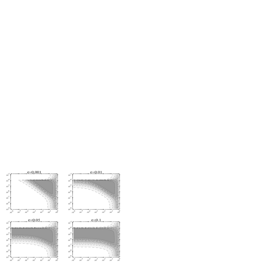
$\sin^{2}2\theta$

Figure 1: The MSW-contours for $\varepsilon=\epsilon_{e}>0$ at one discrete energy ($E_{\nu}=7$ MeV). The shading indicates the value of the survival probability $P_{N}(\nu_{e}\to\nu_{e})$ in the $\sin^{2}2\theta-\Delta$ plane: White corresponds to $0.9\leq P_{N}\leq 1.0$ and the darkest area corresponds to $0.0\leq P_{N}\leq 0.1$.

We have plotted the survival probability $P_{N}(\nu_{e}\to\nu_{e})$ of Eq. (8) in the $\Delta-\sin^{2}2\theta$ plane for a fixed energy $E$ and different values of $\epsilon_{e}$. (See Fig. 1 for positive and Fig. 2 for negative $\epsilon_{e}$, the shading indicates the value of $P_{N}$: White corresponds to $0.9\leq P_{N}\leq 1.0$ and the darkest area corresponds to $0.0\leq P_{N}\leq 0.1$.) For $|\epsilon_{e}|$ as small as $0.001$ the effects of NP are minor (compared to any standard MSW-plot). However already for $|\epsilon_{e}|=0.01$ the triangular shape is distorted and the originally diagonal band appears bent and – most striking – has a “gap” for negative $\epsilon_{e}$. For even larger $|\epsilon_{e}|$ these features remain, only the gap moves towards larger $\sin^{2}2\theta$. Our goal is to understand why these changes arise.

Note that for a given $E_{NA}$ and small vacuum mixing angle we have $\Delta\propto 1/|\sin 2\theta+2\epsilon_{e}\cos 2\theta|^{2}$. For $\epsilon_{e}=0$ this yields the diagonal contours in a double-logarithmic plot in the $\Delta-\sin^{2}2\theta$ plane known as the non-adiabatic band. However for non-vanishing $\epsilon_{e}$ these contours are not diagonal, since $\Delta$ is not proportional to $\sin^{2}2\theta$ anymore. For $\epsilon_{e}>0$ the contours are below the original diagonals and approach a constant for $\sin^{2}2\theta\to 0$. For $\epsilon_{e}<0$ the behavior of the non-adiabatic band is more complicated. For large mixing the new contours are above the standard diagonal and diverge at

$$\tan 2\theta_{div}=-2\epsilon_{e},$$ (13)

where the correction-factor $|1+2\epsilon_{e}\cot 2\theta|^{2}$ vanishes and hence also $E_{NA}(\epsilon_{e})=\gamma_{N}=0$. This implies that – independently of $\Delta$ – almost all the electron neutrinos which were produced above the resonance mainly as the heavier mass eigenstate will “cross over” at the resonance to the lighter mass eigenstate and therefore leave the sun as electron neutrinos. Hence the survival probability is very large, which explains why the contours split at $\sin^{2}2\theta_{div}$. Due to the absolute value in Eq. (12), the contours are symmetric in the region around $\sin^{2}2\theta_{div}$. For very small vacuum mixing $\sin^{2}2\theta\ll\sin^{2}2\theta_{div}$ the contours approach the same constant values as in the case of positive $\epsilon_{e}$.

To understand how the contours split it is instructive to display the survival probability (8) as a function of the energy $E$ for fixed $\sin^{2}2\theta$ and $\Delta$ as shown in Fig. 3. The solid curves show $P_{N}(E)$ for some negative $\epsilon_{e}$, while the dashed curves indicate $P_{N}(E)$ for $\epsilon_{e}=0$. Note that when $\epsilon_{e}$ approaches the value where $\sin^{2}2\theta\simeq\sin^{2}2\theta_{div}$, the “valley” disappears – due to the decrease of the non-adiabatic threshold $E_{NA}(\epsilon_{e})$ – and hence almost all electron neutrinos survive. Also note that the left side of the valley corresponding to the adiabatic threshold is almost unaffected by NP interactions. Thus the adiabatic (horizontal) solution is not shifted. Moreover if the vacuum mixing is large ($\sin^{2}2\theta\approx\tan^{2}2\theta\gg\epsilon_{e}$) then the NP correction factor becomes negligible ($|1+2\epsilon_{e}\cot 2\theta|^{2}\simeq 1$) with the result that the large-angle solution is inert to NP.

4 Solar Neutrino Experiments and $\nu_{e}-e$ FCNCs

Once we have found the new survival probability $P_{N}(E)$ [see (8)], it is straightforward to predict the effects of NP on the MSW-plots for the three kinds of SN experiments in the presence of NP. In order to obtain the suppression rate $\rho$ at any point in the $\Delta-\sin^{2}2\theta$ plane the survival probability $P_{N}(E)$ has to be convoluted with the neutrino energy spectrum times the sensitivity of each experiment. (For all plots we use the SSM predictions of Ref. [19] (including Helium and heavy metal fusion) and the experimental results as summarized in Table I of Ref. [7]. We neglect day-night effects [22].) Fig. 4 shows the contours for $\epsilon_{e}=\pm 0.05$ for Kamiokande, Homestake and the Gallium experiments, respectively. The plots exhibit basically the same behavior as those we showed for a discrete energy (Fig. 1 and Fig. 2). The only difference is the distortion produced by the energy spectrum, as known from the standard MSW-effect.

Finally we have plotted the allowed regions determined by the ratio $\rho$ between the expected and measured neutrino fluxes for the three types of SN experiments. We present the individual 95% C.L. contours (dotted for the combined gallium experiments, dashed for the Homestake and solid for the Kamiokande experiment) together with the combined allowed regions (shaded) for positive and negative $\epsilon_{e}$ in Fig. 5 and Fig. 6, respectively. For very small $\epsilon_{e}=\pm 0.001$ and $\epsilon_{e}=\pm 0.01$ the small-angle solution appears a little shifted, but it does not disappear. Note that the NP neutrino interactions do not change the allowed value for the mass difference, which is fixed at $\Delta\approx 10^{-5}\rm eV^{2}$ due to the adiabatic solution of the Gallium experiments. For larger values $\epsilon_{e}=\pm 0.05$ and $\epsilon_{e}=\pm 0.1$ the effects are more dramatic. One can see that for $\epsilon_{e}=\pm 0.05$ the combined allowed regions include all vacuum mixing angles for which $\sin^{2}2\theta\ \hbox to0.0pt{\raise 3.0pt\hbox{$<$}\hss}{\lower 3.0pt\hbox{$\sim$}}\ 3\times 10^{-4}$. This means in particular that in the presence of NP interactions there may be a solution to the SN problem with vanishingly small vacuum mixing. Moreover for $\epsilon_{e}=-0.05$ there appears a second solution at $\sin^{2}2\theta\simeq 3\times 10^{-2}$, which is due to the gap for negative $\epsilon_{e}$. Finally for $\epsilon_{e}=+0.1$ there is no overlap of the small-angle allowed regions, while for $\epsilon_{e}=-0.1$ there are two solutions at $\sin^{2}2\theta\simeq 10^{-2}$ and $\sin^{2}2\theta\simeq 7\times 10^{-2}$ on both sides of the gap. Moreover – as we expected – the large-angle solution ($\sin^{2}2\theta\simeq 0.6-1.0$ and $\Delta\simeq 3\times 10^{-6}-10^{-4}~{}{\rm eV}^{2}$) is inert to NP for all $\epsilon_{e}$.

5 FCNCs in the Quark Sector

So far we have restricted our discussion to the case of purely leptonic interactions. However electron neutrinos which have been produced in the core of the sun may as well scatter off protons and neutrons when propagating to the solar surface. Without NP interactions this only gives rise to additional weak neutral currents via $Z$-exchange which do not alter the resonant conversion. But in the presence of NP there can be FDNCs and FCNCs which may affect the neutrino propagation. We only consider flavor changing neutrino interactions which correspond to non-vanishing $\epsilon_{u}$ and/or $\epsilon_{d}$ in (3). In this case a new parameter, the ratio $R\equiv N_{n}/N_{p}$ plays a role. If $R$ were constant, we would only need to replace $\epsilon_{e}$ of Section 3 by

$$\epsilon(R)=\epsilon_{e}+2\epsilon_{u}+\epsilon_{d}+(\epsilon_{u}+2\epsilon_{d})~{}R$$ (14)

and could then use all the results we obtained so far. However $R$ is in fact not a constant, but changes from a value of about $0.48$ at the center of the sun to $0.16$ at its surface according to the SSM predictions [5]. Taking into account that ⁴He is four times heavier than ¹H and neglecting the contributions from heavier elements, whose abundances are much smaller, we obtain that

$$R\simeq\frac{X(^{4}{\rm He})}{2X(^{1}{\rm H})+X(^{4}{\rm He})}.$$ (15)

The isotopic abundances $X(^{1}$H) and $X(^{4}$He), the ratio $R$ and the electron density $N_{e}$ are shown as functions of the distance to the solar center $d_{c}$ (in units of the solar radius) in Fig. 7. In the following we discuss the subtleties that arise due to the fact that $R$ is a function of the distance to the solar center.

In order to find the adiabaticity parameter $\gamma_{N}$ [see Eq. (10)] we have to calculate

$$\frac{d{\theta}_{N}}{dx}={\left(\frac{d{\tan 2\theta}_{N}}{d{\theta}_{N}}\right)}^{-1}\left(\frac{d{\tan 2\theta}_{N}}{dx}\right).$$ (16)

Taking the derivative with respect to $x$ (henceforth denoted by a prime) we find that

$$\frac{d{\tan 2\theta}_{N}}{dx} = \frac{d}{dx}\left(\frac{\Delta\sin 2\theta+B}{\Delta\cos 2\theta-A}\right)$$ (17)

$$= \frac{B^{\prime}(\Delta\cos 2\theta-A)-(\Delta\sin 2\theta+B)(-A^{\prime})}{(\Delta\cos 2\theta-A)^{2}}.$$

Computing

$$B^{\prime} = 4E\sqrt{2}G_{F}N_{e}^{\prime}\left[\epsilon_{e}+2\epsilon_{u}+\epsilon_{d}+\left(\epsilon_{u}+2\epsilon_{d}\right)R(x)\right]+$$ (18)

$$4E\sqrt{2}G_{F}N_{e}\left[\left(\epsilon_{u}+2\epsilon_{d}\right)R^{\prime}(x)\right]$$

one can see that a priori $B^{\prime}$ is not proportional to $A^{\prime}$ as in the case of purely leptonic NP, due to its dependence on $R(x)$. But to a very good approximation the second term in (18) can be neglected, since the change of the ratio $R$ between neutron and proton density is much smaller than the change of the electron density, i.e. $R^{\prime}(x)\ll N_{e}^{\prime}/N_{e}$ (see Fig. 7). Then $B^{\prime}$ does not depend on $N_{e}$, but only on $N_{e}^{\prime}$ (like $A^{\prime}$) and we obtain that

$$B=2\epsilon(R)A\hskip 39.83368pt\mbox{and}\hskip 39.83368ptB^{\prime}=2\epsilon(R)A^{\prime},$$ (19)

where $\epsilon(R)$ is defined in Eq. (14). Hence we have recovered the same formal relation between the parameters $A$ and $B$ as in the case of purely leptonic NP, only that now the proportionality factor depends on the distance $x$ traveled by the neutrino. For the adiabaticity parameter $\gamma_{N}$, which is defined at the resonance, this implies that we can take over our previous result (10) (since now $B^{\prime}A=BA^{\prime}$) provided that we replace $\epsilon_{e}$ by $\epsilon(R_{res})$:

$$\gamma_{N}(R)=\gamma|1+2\epsilon(R_{res})\cot 2\theta|^{2}$$ (20)

The position of the resonance for a neutrino produced in the center of the sun depends on its energy. We have to compute $R_{res}$ as a function of the critical density which is given by

$$N_{e}^{crit}=\frac{\Delta\cos 2\theta}{2\sqrt{2}G_{F}(E_{\nu})_{prod}}.$$ (21)

Thus the new adiabaticity parameter $\gamma_{N}(R)$ introduces an additional energy dependence which is however not large since $R<\frac{1}{2}$. Fig. 8 shows $R$ as a function of the electron density $N_{e}$. The dashed curve is a fit to the data points from Ref. [5] by a parabola

$$R(y)\simeq 0.1624-0.0851y+0.4227y^{2},$$ (22)

where $y\equiv N_{e}/(100N_{A})$ and $N_{A}=6.023\times 10^{23}$ is the Avogadro number.

The effects of NP neutrino interactions enter the survival probability $P_{N}(E)$ [see (8)] via the crossing probability $P_{c}$ [through $\gamma_{N}(R)$] and via the matter mixing $\cos 2\theta_{N}$ [see (6)]. For $P_{c}$ we have to calculate $B$ (and therefore $R$) at the resonance which gives rise to the additional energy dependence as discussed above. The factor $\cos 2\theta_{N}$ in (8) has to be taken at the production point of the neutrino. For the intermediate and high-energy neutrinos, which are mainly produced close to the solar center, we have $R_{prod}\simeq 0.4-0.5$. Only for the low-energy neutrinos, a substantial fraction is produced with $R_{prod}<0.4$.

To summarize: To a good approximation all FCNC-effects due to quarks on the neutrino propagation may be accounted for by replacing $\epsilon_{e}$ with $\epsilon(R_{res})$ in the crossing probability $P_{c}$ and with $\epsilon(R_{prod})$ in $\cos 2\theta_{N}$. The change in $P_{c}$ introduces a further energy dependence which is due to the fact that $R_{res}$ depends on the neutrino production energy.

6 Solar Neutrino Experiment and FCNCs in the Quark Sector

In this section we present the MSW-contours and the combined allowed regions for the three types of solar neutrino experiments in the presence of FCNCs in the quark sector. We have used the same method as described previously, only that now we have included the necessary corrections due to the energy dependence of the ratio $R=N_{n}/N_{p}$. We have investigated the three cases of having

• only $\nu-u$ FCNC $(\varepsilon\equiv\epsilon_{u}\neq\epsilon_{d}=0)\Longrightarrow\epsilon(R)=\varepsilon(2+R)$

• only $\nu-d$ FCNC $(\varepsilon\equiv\epsilon_{d}\neq\epsilon_{u}=0)\Longrightarrow\epsilon(R)=\varepsilon(1+2R)$

• both $\nu-u$ FCNC and $\nu-d$ FCNC $(\varepsilon\equiv\epsilon_{d}=\epsilon_{u}\neq 0)\Longrightarrow\epsilon(R)=3\varepsilon(1+R)$.

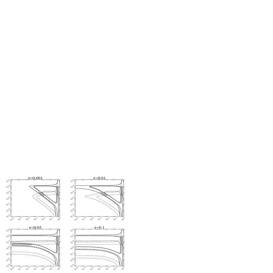
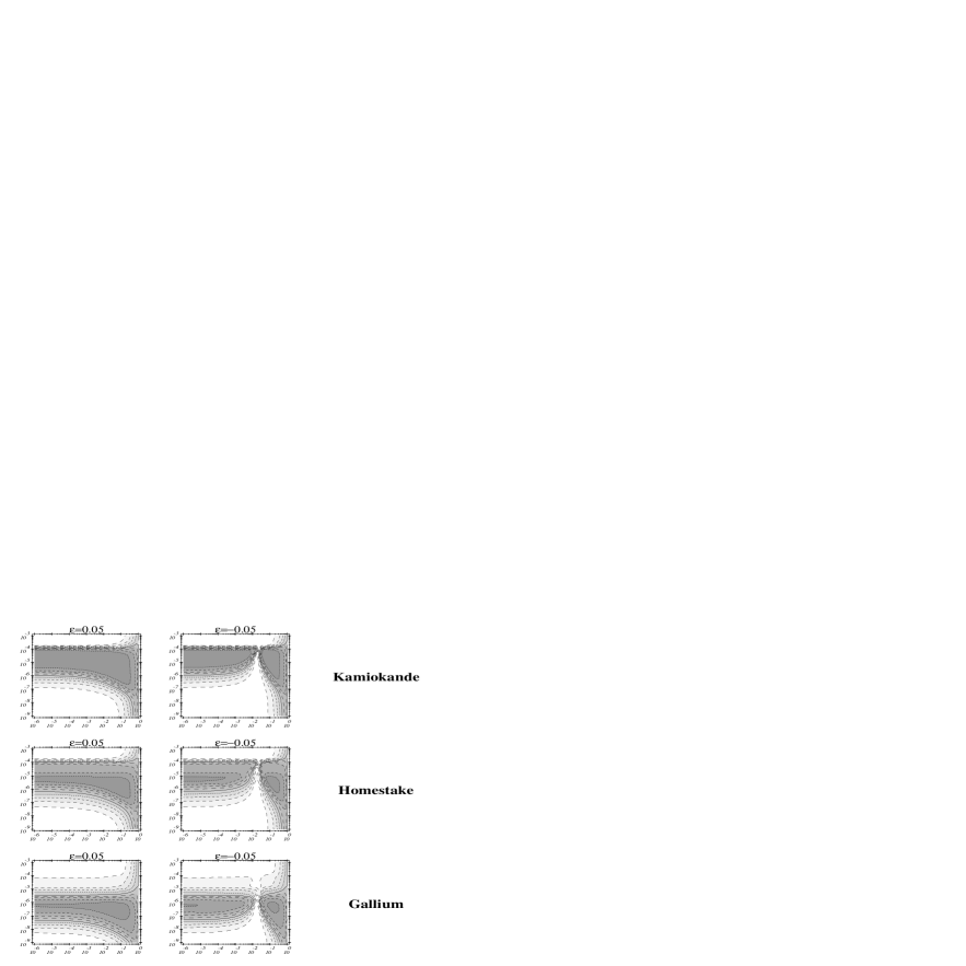
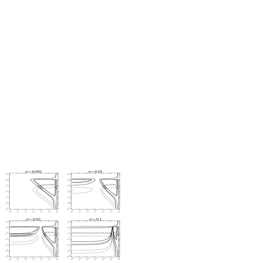
$\sin^{2}2\theta$

Figure 5: The combined allowed regions for the solar neutrino experiments with $\varepsilon=\epsilon_{e}>0$. The dotted contours correspond to the combined gallium experiments, the dashed contours to the Homestake experiment and the solid contours to the Kamiokande experiment. The shaded areas indicate the 95% C.L. combined allowed regions in the $\sin^{2}2\theta-\Delta$ plane.

$\Delta$ [eV²]

$\sin^{2}2\theta$

Figure 6: The combined allowed regions for the solar neutrino experiments with $\varepsilon=\epsilon_{e}<0$. The dotted contours correspond to the combined gallium experiments, the dashed contours to the Homestake experiment and the solid contours to the Kamiokande experiment. The shaded areas indicate the 95% C.L. combined allowed regions in the $\sin^{2}2\theta-\Delta$ plane.

Figure 7: The isotopic abundances $X(^{1}$H) and $X(^{4}$He), the ratio $R=N_{n}/N_{p}$ and the electron density $N_{e}$ (in units of $N_{A}$) as functions of the distance to the solar center $d_{c}$ (in units of the solar radius). The data is taken from Ref. [5].

Figure 8: The ratio $R=N_{n}/N_{p}$ as a function of the electron density $N_{e}$ (in units of $N_{A}$). The solid curve corresponds to the data from Ref. [5] and the dashed curve represents the fit to a parabola.

$\Delta$ [eV²]

$\sin^{2}2\theta$

Figure 9: The MSW-contours for the three types of SN experiments for $\varepsilon\equiv\epsilon_{u}=\pm 0.05$ and $\epsilon_{d}=0$. The shading indicates the value of the suppression ratio $\rho$ in the $\sin^{2}2\theta-\Delta$ plane: White corresponds to $0.9\leq\rho\leq 1.0$ and the darkest area corresponds to $0.0\leq\rho\leq 0.1$

$\Delta$ [eV²]

$\sin^{2}2\theta$

Figure 10: The MSW-contours for the three types of SN experiments for $\varepsilon\equiv\epsilon_{d}=\pm 0.05$ and $\epsilon_{u}=0$. The shading indicates the value of the suppression ratio $\rho$ in the $\sin^{2}2\theta-\Delta$ plane: White corresponds to $0.9\leq\rho\leq 1.0$ and the darkest area corresponds to $0.0\leq\rho\leq 0.1$

As an example for the MSW-contours we show in Fig. 9, Fig. 10 and Fig. 11 our results for the three types of solar neutrino experiments with $\epsilon_{u}=\pm 0.05$, $\epsilon_{d}=\pm 0.05$ and $\epsilon_{u}=\epsilon_{d}=\pm 0.05$, respectively. Comparing with the contours for $\epsilon_{e}$ (see Fig. 4) one can see that for positive $\varepsilon$ the changes are minor, while for negative $\varepsilon$ the region where the contours are split (at $\theta_{div}$) is somewhat tilted. This results from the fact that the effective $\epsilon(R)$ of Eq. (14) is energy dependent. Thus the position of the gap $\sin\theta_{div}$ is not fixed, but varies as a function of $\Delta$. Since $N_{e}^{crit}\propto\Delta$, for larger $\Delta$ also $R(N_{e}^{crit})$ is larger [see Eqs. (21) and (22)]. This slightly increases $\sin\theta_{div}$ [according to (13) with $\epsilon_{e}$ replaced by $\epsilon(R)$] when $\Delta$ takes larger values. This effect is most pronounced for $\varepsilon\equiv\epsilon_{d}$ (see Fig. 10), since in this case the relative change in $\epsilon(R)=\epsilon_{d}(1+2R)$ due to $R$ is most significant.

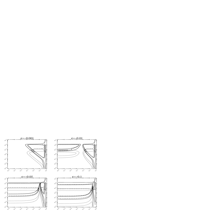
$\sin^{2}2\theta$

Figure 13: The combined allowed regions for the solar neutrino experiments with $\varepsilon\equiv\epsilon_{d}<0$ and $\epsilon_{u}=0$. The dotted contours correspond to the combined gallium experiments, the dashed contours to the Homestake experiment and the solid contours to the Kamiokande experiment. The shaded areas indicates the 95% C.L. combined allowed regions in the $\sin^{2}2\theta-\Delta$ plane.

$\Delta$ [eV²]

$\sin^{2}2\theta$

Figure 14: The combined allowed regions for the solar neutrino experiments with $\varepsilon\equiv\epsilon_{u}=\epsilon_{d}<0$. The dotted contours correspond to the combined gallium experiments, the dashed contours to the Homestake experiment and the solid contours to the Kamiokande experiment. The shaded areas indicates the 95% C.L. combined allowed regions in the $\sin^{2}2\theta-\Delta$ plane.

As the changes in the contours due to the energy dependence of $\epsilon(R)$ are small also the combined allowed regions for the three cases of FCNCs in the quark sector do not differ significantly from the results we obtained in the case of having only $\nu-e$ FCNC. The individual and combined allowed regions at 95% C.L. are shown in Fig. 12, Fig. 13 and Fig. 14 for some negative $\varepsilon$. Again we have the interesting phenomena that for a certain $\varepsilon$ there exist solutions to the SN Problem with vanishingly small vacuum mixing. This occurs for $\epsilon_{u}=\pm 0.02$, $\epsilon_{d}=\pm 0.03$ and $\epsilon_{u}=\epsilon_{d}=\pm 0.01$, respectively. (For positive $\varepsilon$ the qualitative behavior of the contours is similar to that of $\epsilon_{e}>0$ as shown in Fig. 5. For very small $\sin^{2}2\theta$ the contours coincide with those of negative $\varepsilon$.) Note that for $\varepsilon\equiv\epsilon_{u}=\epsilon_{d}=-0.1$ the effective $\epsilon(R)\simeq 0.35-0.45$ is so large that also the large angle solution is affected.

7 Conclusions and Discussion

We have studied the effects of FCNCs on the resonant conversion of solar neutrinos. Our main results are presented in Fig. 5, Fig. 6, Fig. 12, Fig. 13 and Fig. 14. We learn that the changes to the MSW-solution could be dramatic for a NP coupling strength $G_{N}\ \hbox to0.0pt{\raise 3.0pt\hbox{$>$}\hss}{\lower 3.0pt\hbox{$\sim$}}\ 10^{-2}G_{F}$, in particular if the sign of $G_{N}$ is negative.

There remains a question of whether couplings in the relevant range can arise in explicit models of NP. Left-Right symmetric models [8] and supersymmetric models without $R$-parity [9] give rise to the purely leptonic flavor changing neutrino scattering $\nu_{e}e\to\nu_{\ell}e$ ($\ell=\mu,\tau$). However model-independently these reactions are related by $SU(2)_{L}$-rotations to the SM-forbidden decays $\ell^{\pm}\to e^{\pm}e^{\pm}e^{\mp}$. The experimental bounds on the branching ratios (BR) of these reactions [23] (BR$(\mu\to 3e)<10^{-12}$ and BR$(\tau\to 3e)<3.3\times 10^{-6}$) imply that $\epsilon_{e}\ \hbox to0.0pt{\raise 3.0pt\hbox{$<$}\hss}{\lower 3.0pt\hbox{$\sim$}}\ 10^{-6}$ for $\ell=\mu$ and $\epsilon_{e}\ \hbox to0.0pt{\raise 3.0pt\hbox{$<$}\hss}{\lower 3.0pt\hbox{$\sim$}}\ 10^{-3}$ for $\ell=\tau$. Since we found in Section 4 that for $\epsilon_{e}\ \hbox to0.0pt{\raise 3.0pt\hbox{$<$}\hss}{\lower 3.0pt\hbox{$\sim$}}\ 10^{-3}$ the modifications to the MSW-contours are very small (see Fig. 5 and Fig. 6), we conclude that the purely leptonic FCNC effects on the MSW-mechanism (in particular for $\ell=\mu$) are not likely to be significant for solar neutrinos.

For the semi-hadronic neutrino scattering $\nu_{e}q\to\nu_{\ell}q$ the $\nu_{e}\to\nu_{\mu}$ transitions are severely constrained by the decay $\mu\to e\gamma$. The experimental bound [23], BR$(\mu\to e\gamma)<4.9\times 10^{-11}$, implies $\epsilon_{q}\ \hbox to0.0pt{\raise 3.0pt\hbox{$<$}\hss}{\lower 3.0pt\hbox{$\sim$}}\ 10^{-6}$ ruling out significant changes to the MSW-solution. However for $\nu_{e}\to\nu_{\tau}$ oscillations the most stringent bound comes from BR$(\tau\to\rho^{0}e)<4.2\times 10^{-6}$, which is much weaker and gives $\epsilon_{q}\ \hbox to0.0pt{\raise 3.0pt\hbox{$<$}\hss}{\lower 3.0pt\hbox{$\sim$}}\ 10^{-2}$. We note that a relaxation to our estimated bounds on $\epsilon_{f}$ could be achieved by $SU(2)_{L}$ breaking effects. However, since we consider NP at or above the electro-weak scale, the effective four-Fermi couplings related to $\nu_{e}f\to\nu_{\ell}f$ and $\ell\to f\bar{f}e$ differ at most by a factor of a few.

We conclude that for $\nu_{e}q\to\nu_{\tau}q$, the strength of the coupling in NP models could be in the range where it gives interesting effects for solar neutrinos. Supersymmetry without $R$-parity is an example of a model where such a coupling (for $q=d$) exists. In view of the interesting results presented in Ref. [14] and in this work, a detailed analysis of the bounds on flavor changing and new flavor diagonal neutrino interactions in such models is called for.

Acknowledgments

I am indebted to Y. Nir and Y. Grossman for many useful discussions and valuable comments on the manuscript. I also thank E. Nardi for his comments and J.N. Bahcall for useful communications.

$\Delta$ [eV²]

$\Delta$ [eV²]

$\sin^{2}2\theta$

Figure 2: The MSW-contours for $\varepsilon=\epsilon_{e}<0$ at one discrete energy ($E_{\nu}=7$ MeV). The shading indicates the value of the survival probability $P_{N}(\nu_{e}\to\nu_{e})$ in the $\sin^{2}2\theta-\Delta$ plane: White corresponds to $0.9\leq P_{N}\leq 1.0$ and the darkest area corresponds to $0.0\leq P_{N}\leq 0.1$.

$P_{N}(E)$

    $E$ [MeV]

Figure 3: The survival probability $P_{N}(E)$ for different $\varepsilon=\epsilon_{e}$ ($\sin^{2}2\theta=0.005$, $\Delta=3\times 10^{-5}\rm eV^{2}$). The solid curves correspond to $\varepsilon$ as indicated above the plot and the dashed curves correspond to $\varepsilon=0$.

$\Delta$ [eV²]

$\sin^{2}2\theta$

Figure 4: The MSW-contours for the three types of SN experiments with $\varepsilon\equiv\epsilon_{e}=\pm 0.05$. The shading indicates the value of the suppression ratio $\rho$ in the $\sin^{2}2\theta-\Delta$ plane: White corresponds to $0.9\leq\rho\leq 1.0$ and the darkest area corresponds to $0.0\leq\rho\leq 0.1$.

$\Delta$ [eV²]

$\Delta$ [eV²]

$\sin^{2}2\theta$

Figure 11: The MSW-contours for the three types of SN experiments for $\varepsilon\equiv\epsilon_{u}=\epsilon_{d}=\pm 0.05$. The shading indicates the value of the suppression ratio $\rho$ in the $\sin^{2}2\theta-\Delta$ plane: White corresponds to $0.9\leq\rho\leq 1.0$ and the darkest area corresponds to $0.0\leq\rho\leq 0.1$

$\Delta$ [eV²]

$\sin^{2}2\theta$

Figure 12: The combined allowed regions for the solar neutrino experiments with $\varepsilon\equiv\epsilon_{u}<0$ and $\epsilon_{d}=0$. The dotted contours correspond to the combined gallium experiments, the dashed contours to the Homestake experiment and the solid contours to the Kamiokande experiment. The shaded areas indicates the 95% C.L. combined allowed regions in the $\sin^{2}2\theta-\Delta$ plane.

$\Delta$ [eV²]

References

• [1] L. Wolfenstein, Phys. Rev. D 17 (1978) 2369;
S. P. Mikheyev and A. Yu. Smirnov, Yad Fiz. 42 (1985) 1441.
• [2] S. J. Parke, Phys. Rev. Lett. 57 (1986) 1275.
• [3] For a review on neutrino oscillations see e.g.:
T. K. Kuo and J. Pantaleone, Rev. Mod. Phys. 61, No. 4 (1989) 937.
• [4] V. Barger, R. J. N. Phillips and K. Whisnant, Phys. Rev. D 43 (1991) 1110.
• [5] J. N. Bahcall, Neutrino Astrophysics (Cambridge University Press, Cambridge, England, 1989).
• [6] P. Langacker, hep-ph/9411339.
• [7] N. Hata and P. Langacker, hep-ph/9705339.
• [8] J. C. Pati and A. Salam, Phys. Rev. D 10 (1974) 275;
R. N. Mohapatra and J. C. Pati, Phys. Rev. D 11 (1975) 566 and 2558;
R. N. Mohapatra and G. Senjanović, Phys. Rev. D 12 (1975) 1502.
• [9] C. S. Aulakh and N. R. Mohapatra, Phys. Lett. B 119 (1983) 136;
F. Zwirner, Phys. Lett. B 132 (1983) 103;
L. J. Hall and M. Suzuki, Nucl. Phys. B 231 (1984) 419;
J. Ellis et al., Phys. Lett. B 150 (1985) 142;
G. G. Ross and J. W. F. Valle, Phys. Lett. B 151 (1985) 375;
R. Barbieri and A. Masiero, Phys. Lett. B 267 (1986) 679. See also Ref. [12] and references therein.
• [10] E. Roulet, Phys. Rev. D 44 (1991) 935.
• [11] M.M. Guzzo, M. Masiero and S.T. Petcov, Phys. Lett. B 260 (1991) 154.
• [12] V. Barger, R. J. N. Phillips and K. Whisnant, Phys. Rev. D 44 (1991) 1629.
• [13] G. L. Fogli and E. Lisi, Astroparticle Physics 2 (1994) 91.
• [14] P. I. Krastev and J. N. Bahcall, hep-ph/9703267.
• [15] R. Davis, et al., Phys. Rev. Lett. 20, (1968) 1205;
R. Davis, Prog. Part. Nucl. Phys. 32 (1994) 13;
B. T. Cleveland et al., Nucl. Phys. B (Proc. Suppl.) 38 (1995) 47;
K. Lande, to be published in Neutrino 96, Proceedings of the 17th International Conference on Neutrino Physics and Astrophysics, Helsinki, Finland, 13–19 June 1996, edited by K. Huitu, K. Enqvist and J. Maalampi (World Scientific, Singapore).
• [16] K. S. Hirata, et al., Phys. Rev. Lett. 62 (1989) 16;
Y. Fukuda et al. (Kamiokande Collaboration), Phys. Rev. Lett. 77 (1996) 1683.
• [17] P. Anselmann et al., Phys. Lett. B 285 (1992) 390, 327 (1994) 377, 342 (1995) 440, 357 (1995) 237;
T. Kirsten et al. (GALLEX Collaboration), to be published in Neutrino 96, Proceedings of the 17th International Conference on Neutrino Physics and Astrophysics, Helsinki, Finland, 13–19 June 1996, edited by K. Huitu, K. Enqvist and J. Maalampi (World Scientific, Singapore).
• [18] A. I. Abasov et al., Phys. Rev. Lett. 67 (1991) 3332;
J. N. Abdurashitov et al., Phys. Lett. B 328 (1994) 234;
V. Gavrin et al. (SAGE Collaboration), to be published in Neutrino 96, Proceedings of the 17th International Conference on Neutrino Physics and Astrophysics, Helsinki, Finland, 13–19 June 1996, edited by K. Huitu, K. Enqvist and J. Maalampi (World Scientific, Singapore).
• [19] J. N. Bahcall and M. H. Pinsonneault, Rev. Mod. Phys. 67, 781 (1995).
• [20] Y. Grossman, Phys. Lett. B 359 (1995) 141, (hep-ph/9507344).
• [21] S. T. Petcov, Phys. Lett. B 200 (1988) 373;
see also: Nucl. Phys. B (Proc. Suppl.) 13 (1990) 527.
• [22] J. N. Bahcall and P. I. Krastev, hep-ph/9706239.
• [23] R. M. Barnett et al., Particle Data Group, Phys. Rev. D 54 (1996).