DTP/97/26

July 1997

A complete ${\cal O}(\alpha\alpha_{s})$ calculation of the
Photon + 1 Jet Rate in $e^{+}e^{-}$ annihilation
A. Gehrmann–De Ridder and E. W. N. Glover
Physics Department, University of Durham,
Durham DH1 3LE, England

We present a complete calculation of the photon + 1 jet rate in $e^{+}e^{-}$ annihilation up to ${\cal O}(\alpha\alpha_{s})$. Although formally of next-to-leading order in perturbation theory, this calculation contains several ingredients appropriate to a next-to-next-to-leading order calculation of jet observables. In particular, we describe a generalization of the commonly used phase space slicing method to isolate the singularities present when more than one particle is unresolved. Within this approach, we analytically evaluate the singularities associated with the following double unresolved regions; triple collinear, soft/collinear and double single collinear configurations as well as those from the collinear limit of virtual graphs. By comparing the results of our calculation with the existing data on the photon + 1 jet rate from the ALEPH Collaboration at CERN, we make a next-to-leading order determination of the process-independent non-perturbative quark-to-photon fragmentation function $D_{q\to\gamma}(z,\mu_{F})$ at ${\cal O}(\alpha\alpha_{s})$. As a first application of this measurement allied with our improved perturbative calculation, we determine the dependence of the isolated photon + 1 jet cross section in a democratic clustering approach on the jet resolution parameter $y_{\rm cut}$ at next-to-leading order. The next-to-leading order corrections to this observable are moderate but improve the agreement between theoretical prediction and experimental data.

1 Introduction

Although the production dynamics of photons and of jets are both individually well understood theoretically, their interplay is not. Hadronic jets are initiated by the production of quarks and gluons which subsequently fragment into clusters of hadrons. In events where a photon is produced in addition to the jets, this photon can have two possible origins: the direct radiation of a photon off a primary quark and the fragmentation of a hadronic jet into a photon carrying a sizeable fraction of the jet energy. While the former direct process can be calculated within the framework of the Standard Model, the latter is described by the process-independent quark-to-photon and gluon-to-photon fragmentation functions [1], which cannot be calculated using perturbative methods but have to be determined from experimental data.

Directly emitted photons are usually well separated from all hadron jets produced in a particular event, while photons originating from fragmentation processes are primarily to be found inside hadronic jets. Consequently, by imposing some isolation criterion on the photon, one is in principle able to suppress (but not to eliminate) the fragmentation contribution to final state photon cross sections, and thus to define isolated photons. However, recent analyses of the production of isolated photons in electron-positron and proton-antiproton collisions have shown that the application of a geometrical isolation cone surrounding the photon does not lead to a reasonable agreement between theoretical prediction and experimental data. This discrepancy has important consequences. Data on high $p_{T}$ photon production are commonly used to extract informations on the gluon distribution in the proton [2]. Furthermore, the understanding of final state photon radiation in proton-proton collisions is even more crucial for searches for the two photon decay mode of the Higgs boson at the LHC [3].

An alternative approach to study final state photons produced in a hadronic environment is obtained by applying the so-called democratic clustering procedure [4]. In this approach, the photon is treated like any other hadron and is clustered simultaneously with the other hadrons into jets. Consequently, one of the jets in the final state contains a photon and is labelled ‘photon jet’ if the fraction of electromagnetic energy within the jet is sufficiently large,

$$z=\frac{E_{EM}}{E_{EM}+E_{HAD}}>z_{\rm cut},$$ (1.1)

with $z_{\rm cut}$ determined by the experimental conditions. This photon is called isolated if it carries more than a certain fraction, typically 95%, of the jet energy and said to be non-isolated otherwise. Note that this separation is made by studying the experimental $z$ distribution and is usually such that hadronisation effects, which tend to reduce $z$, are minimized. The cross section for the production of isolated photons defined in this approach thus receives sizeable contributions from both direct photon and fragmentation processes.

Up to now, this democratic procedure has only been applied by the ALEPH collaboration at CERN in an analysis of two jet events in electron-positron annihilation in which one of the jets contains a highly energetic photon [5]. In this analysis, ALEPH made a leading order determination of the quark-to-photon fragmentation function by comparing the photon + 1 jet rate calculated up to ${\cal O}(\alpha)$ [4] with the data. Then, by inserting their measurement into an ${\cal O}(\alpha\alpha_{s})$ calculation of the ‘isolated’ photon + 2 and 3 jet rates, they found good agreement for a wide range of values of the jet resolution parameter $y_{\rm cut}$.

In addition, the ${\cal O}(\alpha)$ ‘isolated’ photon + 1 jet rate agreed well with the ALEPH data. This is remarkable, since with the use of an isolation criterion based on the application of a geometrical cone previously considered [6], the agreement between data and theory for this rate was poor and only improved at the expense of large negative radiative corrections [7, 8, 9, 10]. The main reason for the size and sign of these corrections was due to the exclusion of soft gluons from the cone containing the photon [11].

Recently, we have presented a next-to-leading order determination of the quark to photon fragmentation function [12] based on an ${\cal O}(\alpha\alpha_{s})$ calculation of the photon + 1 jet rate and the ALEPH data. Both theoretical and experimental analyses were performed using a democratic clustering approach; in particular both analyses used the Durham jet recombination algorithm [13]. Not only is the agreement with the ‘isolated’ photon + 1 jet rate improved, but the higher order corrections obtained in this approach were found to be moderate, demonstrating the perturbative stability of this particular photon definition. In this paper, we describe the calculation in more detail. In particular, we extend the commonly used phase space slicing technique [14, 15] developed to isolate the divergences when one of the final state particles is unresolved to situations where two particles are unresolved.

The paper is organized as follows. In section 2 we discuss the general structure of photon + $n$ jet events in electron-positron collisions, with particular emphasis on where the singularities arise and how they are absorbed into the photon fragmentation functions. In this fixed order approach, it is critical that the power counting of the various contributions is correct. One consequence is that the commonly held view [16] that the quark-to-photon fragmentation function is ${\cal O}(\alpha/\alpha_{s})$ is untenable. The particular features of the photon + 1 jet rate are discussed in section 3. We adopt the resolved parton philosophy of [15] and introduce a small parameter $y_{\rm min}$ to separate the final state phase space into resolved and unresolved regions and to isolate the singularities lying in the unresolved regions. Within this approach, it is vital that the various singular regions precisely match onto each other. The evaluation of the associated different divergent contributions to the photon + 1 jet rate is presented in sections 4–7. Fully resolved and single unresolved contributions from the four parton process $\gamma^{*}\to q\bar{q}\gamma g$ are described in section 4 while the double unresolved contributions that arise when, for example, three particles are simultaneously collinear are analytically evaluated in section 5. Contributions from the one-loop process with collinear final state partons are presented in section 6 and the fragmentation contribution is presented in section 7. All divergent contributions are combined in section 8, where we explicitly show that after factorization of collinear singularities, no divergences remain. Although the individual contributions are finite, they do depend on the parameter $y_{\rm min}$. Clearly, the physical cross section cannot depend on $y_{\rm min}$, and in section 9 we numerically show that, provided $y_{\rm min}$ is taken small enough, this is indeed the case. We combine our numerical results with the experimental data in section 10 and determine the next-to-leading order quark-to-photon fragmentation function for two values of $\alpha_{s}(M_{Z})$. Finally, section 11 contains our conclusions.

2 The $n$ jet + photon cross section

Let us first consider the general structure of the $e^{+}e^{-}\to n$ jet + photon cross section, fully differential in all quantities,

$${\rm d}\sigma(n~{}{\rm jets}+``\gamma")={\rm d}\hat{\sigma}_{\gamma}+\sum_{a}{\rm d}\hat{\sigma}_{a}\otimes D^{B}_{a\to\gamma}.$$ (2.1)

There are two contributions, first the ‘prompt’ photon production where the photon is produced directly in the hard interaction and second, the longer distance fragmentation process where one of the partons fragments into a photon and transfers a fraction of the parent momentum to the photon. Each type of parton, $a$, contributes according to the process independent parton-to-photon fragmentation functions $D^{B}_{a\to\gamma}$ and the sum runs over all partons. Note that although the fragmentation functions are non-perturbative, we can nominally assign a power of coupling constants, based on counting the couplings necessary to radiate a photon. Since the photon couples directly to the quark, $D_{q\to\gamma}$ is naively of ${\cal O}(\alpha)$ while the gluon can only couple to the photon via a quark and we might expect that $D_{g\to\gamma}$ is of ${\cal O}(\alpha\alpha_{s})$. This simplistic argument is supported by models of the fragmentation function [17] which suggest that gluon fragmentation is a much smaller effect than quark fragmentation.

The individual terms in eq. (2.1) may be divergent and are denoted by hatted quantities. However, we can reorganise them as follows. In the most general case we have,

$${\rm d}\hat{\sigma}_{\gamma} = {\rm d}\sigma_{\gamma}+\sum_{q}{\rm d}\sigma_{q}\otimes\Gamma_{q\to\gamma}+{\rm d}\sigma_{g}\otimes\Gamma_{g\to\gamma},$$

$${\rm d}\hat{\sigma}_{q} = \sum_{q^{\prime}}{\rm d}\sigma_{q^{\prime}}\otimes\Gamma_{q^{\prime}\to q}+{\rm d}\sigma_{g}\otimes\Gamma_{g\to q},$$

$${\rm d}\hat{\sigma}_{g} = \sum_{q}{\rm d}\sigma_{q}\otimes\Gamma_{q\to g}+{\rm d}\sigma_{g}\otimes\Gamma_{g\to g},$$ (2.2)

where all of the divergences are concentrated in the factorization scale dependent transition functions $\Gamma_{i\to j}$. The sum covers all active quark and antiquark flavours. The process specific cross sections ${\rm d}\sigma_{\gamma}$, ${\rm d}\sigma_{q}$, ${\rm d}\sigma_{g}$ are now finite. Inserting these definitions back into eq. (2.1), yields a physical cross section in terms of finite quantities,

$${\rm d}\sigma(n~{}{\rm jets}+``\gamma")={\rm d}\sigma_{\gamma}+\sum_{q}{\rm d}\sigma_{q}\otimes D_{q\to\gamma}+{\rm d}\sigma_{g}\otimes D_{g\to\gamma}$$ (2.3)

where the physical (and factorization scale dependent) fragmentation functions are given by,

$$D_{q\to\gamma} = \Gamma_{q\to\gamma}+\sum_{q^{\prime}}\Gamma_{q\to q^{\prime}}\otimes D^{B}_{q^{\prime}\to\gamma}+\Gamma_{q\to g}\otimes D^{B}_{g\to\gamma},$$

$$D_{g\to\gamma} = \Gamma_{g\to\gamma}+\sum_{q}\Gamma_{g\to q}\otimes D^{B}_{q\to\gamma}+\Gamma_{g\to g}\otimes D^{B}_{g\to\gamma}.$$ (2.4)

While the singular parts of the transition functions are process independent and well known, it is sometimes convenient to carry some finite perturbative pieces as well [4], so that,

$${\rm d}\sigma_{\gamma}^{R} = {\rm d}\sigma_{\gamma}-\sum_{q}{\rm d}\sigma_{q}\otimes a_{q\to\gamma}-{\rm d}\sigma_{g}\otimes a_{g\to\gamma},$$

$$\Gamma_{q\to\gamma}^{R} = \Gamma_{q\to\gamma}+a_{q\to\gamma},$$

$$\Gamma_{g\to\gamma}^{R} = \Gamma_{g\to\gamma}+a_{g\to\gamma},$$ (2.5)

and to define the ‘effective’ parton-to-photon fragmentation functions,

$${\cal D}_{q\to\gamma} = D_{q\to\gamma}+a_{q\to\gamma},$$

$${\cal D}_{g\to\gamma} = D_{g\to\gamma}+a_{g\to\gamma}.$$ (2.6)

With these modifications that are particularly suited to the resolved parton philosophy [15] we shall employ later on to isolate the singularities in ${\rm d}\hat{\sigma}_{\gamma}$ and ${\rm d}\hat{\sigma}_{a}$, the cross section is given by,

$${\rm d}\sigma(n~{}{\rm jets}+``\gamma")={\rm d}\sigma_{\gamma}^{R}+\sum_{q}{\rm d}\sigma_{q}^{R}\otimes{\cal D}_{q\to\gamma}+{\rm d}\sigma_{g}^{R}\otimes{\cal D}_{g\to\gamma},$$ (2.7)

where the superscript $R$ indicates that the partons are ‘resolved’ [15]. Within the fixed order approach, only the ‘prompt’ photon process contributes at lowest order, and,

$${\rm d}\hat{\sigma}_{\gamma}^{(LO)} = {\rm d}\sigma_{\gamma}^{R(LO)}=\Theta~{}{\rm d}\hat{\sigma}_{0}(n~{}p+\gamma),$$

$${\rm d}\hat{\sigma}_{q}^{(LO)} = 0,$$

$${\rm d}\hat{\sigma}_{g}^{(LO)} = 0.$$ (2.8)

The $n$ parton + photon cross section ${\rm d}\hat{\sigma}_{0}(n~{}p+\gamma)$ is evaluated in the tree approximation and $\Theta$ represents the experimental jet and photon definition cuts. In this way the theoretical cross section can be matched onto the specific experimental details. At this order each parton is identified as a jet and the photon as a photon.

At next-to-leading order, both ‘prompt’ photon production and the quark-to-photon fragmentation process contribute,

$${\rm d}\hat{\sigma}_{\gamma}^{(NLO)} = \Theta\left({\rm d}\hat{\sigma}_{1}(n~{}p+\gamma)+\int{\rm d}\hat{\sigma}_{0}((n+1)~{}p+\gamma)\right),$$

$${\rm d}\hat{\sigma}_{q}^{(NLO)} = \Theta~{}{\rm d}\hat{\sigma}_{0}((n+1)~{}p),$$

$${\rm d}\hat{\sigma}_{g}^{(NLO)} = 0.$$ (2.9)

‘Prompt’ photon production may occur via the one loop virtual corrections to the $n$ parton + photon process ${\rm d}\hat{\sigma}_{1}(n~{}p+\gamma)$ or by the tree level emission of an additional parton ${\rm d}\hat{\sigma}_{0}((n+1)~{}p+\gamma)$. The integral sign represents the integration over the additional phase space variables due to the presence of an extra parton in the final state. The fragmentation contribution arises from the lowest order $n+1$ parton process with one quark fragmenting into a photon. The remaining unfragmented partons are directly identified as jets. Although the physical cross section is finite, individual contributions are divergent. In ${\rm d}\hat{\sigma}_{\gamma}^{(NLO)}$, there are infrared singularities arising from configurations where one of the partons is theoretically ‘unresolved’. For example, the virtual graphs contain singularities due to soft gluons or collinear partons while similar divergences occur in the bremsstrahlung process. The correct treatment of infrared divergences is well known [18, 19] and has been discussed widely in the literature. Many general approaches have been developed to isolate the infrared divergences at next-to-leading order [15, 20, 21, 22]. In [4], the approach of [15] was used to isolate the divergences present in the bremsstrahlung contributions and to combine them with those arising from the virtual graphs. While the leading infrared singularities due to soft gluon emission should cancel within ${\rm d}\hat{\sigma}_{\gamma}^{(NLO)}$, some collinear mass singularities remain. These singularities, which occur as the quark and photon become collinear, are proportional to ${\rm d}\hat{\sigma}_{q}^{(NLO)}$, are factorizable and can be absorbed by a redefinition of the fragmentation function as described above. Working within the $\overline{MS}$ scheme [23], the transition functions for a quark of charge $e_{q}$ are up to ${\cal O}(\alpha)$ given by,

$$\Gamma_{q\to q^{\prime}} = \delta_{qq^{\prime}},$$

$$\Gamma_{q\to\gamma} = \left(\frac{\alpha e_{q}^{2}}{2\pi}\right)\frac{1}{\Gamma(1-\epsilon)}\left(\frac{4\pi\mu^{2}}{\mu_{F}^{2}}\right)^{\epsilon}\,\left[-\frac{1}{\epsilon}P^{(0)}_{q\to\gamma}\right],$$ (2.10)

where $P^{(0)}_{q\to\gamma}$ is the $\epsilon\to 0$ part of the the lowest order splitting function in $(4-2\epsilon)$-dimensions [24],

$$P_{q\to\gamma}(z)=\frac{1+(1-z)^{2}-\epsilon z^{2}}{z}.$$ (2.11)

Here, the variable $z$ represents the fraction of the ‘photon’ energy that is genuinely electromagnetic in origin in the quark-photon cluster.

Each term in the ‘prompt’ photon contribution is finite and may be evaluated numerically,

$${\rm d}\sigma_{\gamma}^{R(NLO)}=\Theta\left({\rm d}\sigma^{R}_{1}(n~{}p+\gamma)+\int{\rm d}\sigma^{R}_{0}((n+1)~{}p+\gamma)\right),$$ (2.12)

where the superscript $R$ indicates that the partons are ‘resolved’ [15]. For the numerical evaluation of the cross section within the resolved parton approach it is moreover useful to identify a universal constant piece and to absorb it into the ‘effective’ fragmentation function [4],

$${\cal D}_{q\to\gamma}(z)=D_{q\to\gamma}(z,\mu_{F})+\left(\frac{\alpha e_{q}^{2}}{2\pi}\right)\left(\log\left(\frac{s_{\rm min}s_{q\bar{q}}z(1-z)}{M^{2}\mu_{F}^{2}}\right)P^{(0)}_{q\to\gamma}(z)+z\right),$$ (2.13)

where M is the mass of the final state and $s_{q\bar{q}}$ is the invariant mass of the radiating quark-antiquark system. We see that the effective quark-to-photon fragmentation function, ${\cal D}_{q\to\gamma}$, depends on the unphysical parton resolution parameter $s_{\rm min}$ introduced to isolate the singularities. Physical cross sections cannot depend on $s_{\rm min}$, and there must be a cancellation between the resolved prompt photon and fragmentation contributions. In ref. [4] this was shown to be the case. The genuine non-perturbative fragmentation function $D_{q\to\gamma}(z,\mu_{F})$ cannot be calculated and needs to be extracted from data.

At next-to-next-to-leading order, the ‘prompt’ photon contribution now contains contributions from the two-loop $n$ parton + photon process, as well as the one-loop $(n+1)$-parton + photon and tree level $(n+2)$-parton + photon processes. Similarly, the quark-to-photon fragmentation term receives contributions from the one-loop $(n+1)$-parton process and the tree level $(n+2)$-parton process, while the gluon-to-photon fragmentation term, appearing for the first time at this order, only receives a contribution from the tree level $(n+1)$-parton process,

$${\rm d}\hat{\sigma}_{\gamma}^{(NNLO)} = \Theta\Biggl{(}{\rm d}\hat{\sigma}_{2}(n~{}p+\gamma)+\int{\rm d}\hat{\sigma}_{1}((n+1)~{}p+\gamma)$$

$$\qquad+\int\int{\rm d}\hat{\sigma}_{0}((n+2)~{}p+\gamma)\Biggr{)},$$

$${\rm d}\hat{\sigma}_{q}^{(NNLO)} = \Theta\left({\rm d}\hat{\sigma}_{1}((n+1)~{}p)+\int{\rm d}\hat{\sigma}_{0}((n+2)~{}p)\right),$$

$${\rm d}\hat{\sigma}_{g}^{(NNLO)} = \Theta\;{\rm d}\hat{\sigma}_{0}((n+1)~{}p).$$ (2.14)

As at next-to-leading order, the singularities present in the ‘prompt’ photon bremsstrahlung and in the fragmentation processes can be isolated. However, unlike at next-to-leading order, there are contributions to the ‘prompt’ photon bremsstrahlung process where two of the final state partons can be simultaneously theoretically unresolved. These contributions are expected to appear in the divergent part of any jet cross section evaluated at next-to-next-to-leading order. In the most general case, the following four double unresolved configurations can occur:

• The triple collinear configuration, where three partons become simultaneously collinear to each other, but none are soft.

• The soft/collinear configuration, where two partons become collinear while a third parton becomes soft.

• The double single collinear configuration, where two distinct, independent pairs of partons become simultaneously collinear.

• The double soft configuration, where two partons become simultaneously soft.

The photon + 1 jet cross section at ${\cal O}(\alpha\alpha_{s})$, calculated in the remainder of this paper, receives only contributions from three of these double unresolved configurations (triple collinear quark-photon-gluon, soft gluon/collinear photon and double single collinear quark-photon/antiquark-gluon) and the corresponding double unresolved factors will be calculated analytically in section 5. There are also singular contributions arising when a gluon is virtual while another parton is collinear or soft. In our calculation, we have only a virtual collinear contribution, studied in section 6, as the photon cannot be soft. Finally, another new class of singularities occurs when together with the remnants of the quark/photon fragmentation cluster an unresolved or virtual gluon is emitted. We will explicitly evaluate this fragmentation contribution in section 7. Having isolated the singular contributions in this way allows us to define finite ‘resolved’ parton cross sections for both ‘prompt’ photon and fragmentation processes which in the most general case reads,

$${\rm d}\sigma_{\gamma}^{R(NNLO)} = \Theta\Biggl{(}{\rm d}\sigma_{2}^{R}(n~{}p+\gamma)+\int{\rm d}\sigma_{1}^{R}((n+1)~{}p+\gamma)$$

$$\qquad+\int\int{\rm d}\sigma_{0}^{R}((n+2)~{}p+\gamma)\Biggr{)},$$

$${\rm d}\sigma_{q}^{R(NNLO)} = \Theta\left({\rm d}\sigma_{1}^{R}((n+1)~{}p)+\int{\rm d}\sigma_{0}^{R}((n+2)~{}p)\right),$$

$${\rm d}\sigma_{g}^{R(NNLO)} = \Theta\;{\rm d}\sigma_{0}^{R}((n+1)~{}p).$$ (2.15)

Each resolved cross section is finite and can be numerically evaluated for arbitrary experimental constraints.

The most singular divergences are due to soft gluon radiation and cancel between the virtual and real processes. However, double and single poles in $\epsilon$ due to collinear singularities remain, whose form is determined by the known next-to-leading order transition functions. Keeping only terms that are necessary to expand eq. (2.2) up to ${\cal O}(\alpha\alpha_{s})$ and bearing in mind that $D_{g\to\gamma}$ is already ${\cal O}(\alpha\alpha_{s})$, then in the $\overline{MS}$–scheme,

$$\Gamma_{q\to\gamma} = \left(\frac{\alpha e_{q}^{2}}{2\pi}\right)\frac{1}{\Gamma(1-\epsilon)}\left(\frac{4\pi\mu^{2}}{\mu_{F}^{2}}\right)^{\epsilon}\,\left[-\frac{1}{\epsilon}P^{(0)}_{q\to\gamma}\right]$$

$$+\left(\frac{\alpha e_{q}^{2}}{2\pi}\right)\left(\frac{\alpha_{s}C_{F}}{2\pi}\right)\frac{1}{\Gamma^{2}(1-\epsilon)}\left(\frac{4\pi\mu^{2}}{\mu_{F}^{2}}\right)^{2\epsilon}\,\left[\frac{1}{2\epsilon^{2}}P^{(0)}_{q\to q}\otimes P^{(0)}_{q\to\gamma}-\frac{1}{2\epsilon}P^{(1)}_{q\to\gamma}\right],$$

$$\Gamma_{g\to\gamma} = \left(\frac{\alpha e_{q}^{2}}{2\pi}\right)\left(\frac{\alpha_{s}T_{R}}{2\pi}\right)\frac{1}{\Gamma^{2}(1-\epsilon)}\left(\frac{4\pi\mu^{2}}{\mu_{F}^{2}}\right)^{2\epsilon}\,\left[\frac{1}{2\epsilon^{2}}\sum_{q}P^{(0)}_{g\to q}\otimes P^{(0)}_{q\to\gamma}-\frac{1}{2\epsilon}P^{(1)}_{g\to\gamma}\right],$$

$$\Gamma_{q\to q^{\prime}} = \left(1+\left(\frac{\alpha_{s}C_{F}}{2\pi}\right)\frac{1}{\Gamma(1-\epsilon)}\left(\frac{4\pi\mu^{2}}{\mu_{F}^{2}}\right)^{\epsilon}\left[-\frac{1}{\epsilon}P^{(0)}_{q\to q}\right]\right)\delta_{qq^{\prime}},$$

$$\Gamma_{g\to q} = \left(\frac{\alpha_{s}T_{R}}{2\pi}\right)\frac{1}{\Gamma(1-\epsilon)}\left(\frac{4\pi\mu^{2}}{\mu_{F}^{2}}\right)^{\epsilon}\left[-\frac{1}{\epsilon}P^{(0)}_{g\to q}\right],$$

$$\Gamma_{q\to g} = 0,$$

$$\Gamma_{g\to g} = 1,$$ (2.16)

where the QCD casimirs $C_{F}$ and $T_{R}$ are,

$$C_{F}=\frac{N^{2}-1}{2N},\qquad T_{R}=\frac{1}{2}.$$

The lowest order quark-to-quark and gluon-to-quark splitting functions are [24],

$$P^{(0)}_{q\to q}(z) = \frac{1+z^{2}}{(1-z)_{+}}+\frac{3}{2}\delta(1-z),$$ (2.17)

$$P^{(0)}_{g\to q}(z) = z^{2}+(1-z)^{2},$$ (2.18)

while the next-to-leading order quark-to-photon and gluon-to-photon splitting functions are given by [25, 26],

$$P^{(1)}_{q\to\gamma}(z) = -\frac{1}{2}+\frac{9}{2}z+\left(-8+\frac{1}{2}z\right)\ln z+2z\ln(1-z)+\left(1-\frac{1}{2}z\right)\ln^{2}z$$ (2.19)

$$+\left[\ln^{2}(1-z)+4\ln z\ln(1-z)+8{\rm Li}_{2}(1-z)-\frac{4}{3}\pi^{2}\right]P^{(0)}_{q\to\gamma}(z),$$

$$P^{(1)}_{g\to\gamma}(z) = -2+6z-\frac{82}{9}z^{2}+\frac{46}{9z}+\left(5+7z+\frac{8}{3}z^{2}+\frac{8}{3z}\right)\ln z+(1+z)\ln^{2}z.$$ (2.20)

The transition functions $\Gamma_{i\to j}$ determine the singularity structure of the bare fragmentation functions up to ${\cal O}(\alpha\alpha_{s})$,

$$D^{B}_{q\to\gamma}(z) = \sum_{q^{\prime}}\Gamma_{q\to q^{\prime}}^{-1}\otimes D_{q^{\prime}\to\gamma}(z,\mu_{F})-\sum_{q^{\prime}}\Gamma_{q\to q^{\prime}}^{-1}\otimes\Gamma_{q^{\prime}\to\gamma}+\Gamma_{q\to g}^{-1}\otimes D_{g\to\gamma}(z,\mu_{F})$$

$$= D_{q\to\gamma}(z,\mu_{F})\,+\left(\frac{\alpha e_{q}^{2}}{2\pi}\right)\frac{1}{\Gamma(1-\epsilon)}\left(\frac{4\pi\mu^{2}}{\mu_{F}^{2}}\right)^{\epsilon}\frac{1}{\epsilon}P^{(0)}_{q\to\gamma}(z)$$

$$+\left(\frac{\alpha_{s}C_{F}}{2\pi}\right)\frac{1}{\Gamma(1-\epsilon)}\left(\frac{4\pi\mu^{2}}{\mu_{F}^{2}}\right)^{\epsilon}\frac{1}{\epsilon}P^{(0)}_{q\to q}\otimes D_{q\to\gamma}(z,\mu_{F})$$

$$+\left(\frac{\alpha e_{q}^{2}}{2\pi}\right)\left(\frac{\alpha_{s}C_{F}}{2\pi}\right)\frac{1}{\Gamma^{2}(1-\epsilon)}\left(\frac{4\pi\mu^{2}}{\mu_{F}^{2}}\right)^{2\epsilon}\;\left[\frac{1}{2\epsilon^{2}}P^{(0)}_{q\to q}\otimes P^{(0)}_{q\to\gamma}+\frac{1}{2\epsilon}P^{(1)}_{q\to\gamma}\right],$$

$$D^{B}_{g\to\gamma}(z) = \Gamma_{g\to g}^{-1}\otimes D_{g\to\gamma}(z,\mu_{F})-\Gamma_{g\to g}^{-1}\otimes\Gamma_{g\to\gamma}+\sum_{q}\Gamma_{g\to q}^{-1}\otimes D_{q\to\gamma}(z,\mu_{F})$$

$$= D_{g\to\gamma}(z,\mu_{F})\,+\sum_{q}\left(\frac{\alpha_{s}T_{R}}{2\pi}\right)\frac{1}{\Gamma(1-\epsilon)}\left(\frac{4\pi\mu^{2}}{\mu_{F}^{2}}\right)^{\epsilon}\frac{1}{\epsilon}P^{(0)}_{g\to q}\otimes D_{q\to\gamma}(z,\mu_{F})$$

$$+\sum_{q}\left(\frac{\alpha_{s}T_{R}}{2\pi}\right)\,\left(\frac{\alpha e_{q}^{2}}{2\pi}\right)\frac{1}{\Gamma^{2}(1-\epsilon)}\left(\frac{4\pi\mu^{2}}{\mu_{F}^{2}}\right)^{2\epsilon}\;\left[\frac{1}{2\epsilon^{2}}P^{(0)}_{g\to q}\otimes P^{(0)}_{q\to\gamma}+\frac{1}{2\epsilon}P^{(1)}_{g\to\gamma}\right],$$

which must absorb the remaining collinear singularities present in the $\gamma+n$ jet cross section at next-to-next-to-leading order. Note that in expanding the perturbative counterterms, we have systematically assumed that the gluon-to-photon fragmentation function is ${\cal O}(\alpha\alpha_{s})$, and therefore does not contribute to $D^{B}_{q\to\gamma}$ at this order.

Concentrating on the evaluation of the photon + 1 jet rate at fixed order, ${\cal O}(\alpha\alpha_{s})$, the production of gluons is suppressed by a power of $\alpha_{s}$ compared to the quark production. Therefore, the contribution from the gluon fragmentation to the photon + 1 jet rate is of ${\cal O}(\alpha\alpha_{s}^{2})$ and must be neglected in a consistent fixed order framework. Consequently, the quark-to-photon fragmentation function alone must absorb the remaining singularities and demanding that this is so provides a powerful check that the singularities have been correctly isolated. This factorization procedure will be explicitly described in section 8. Moreover, we note that evaluating the real double unresolved contributions using a strong ordered approach, i.e. requiring that one unresolved parton is much less unresolved than the other, fails to produce the necessary singularity structure [27].

3 The ‘photon’ + 1 jet cross section

We now concentrate on the case where only a single jet is produced in addition to the ‘photon’. The photon + 1 jet rate in electron-positron annihilation is rather particular, since the leading order process, 1 parton + ‘direct’ photon production, vanishes. The lowest non-vanishing order [4], ${\cal O}(\alpha)$, is therefore equivalent to the next-to-leading order outlined above, where ‘direct’ and fragmentation processes contribute at equal level. This observable is therefore particularly suitable for determining the non-perturbative component of the quark-to-photon fragmentation function.

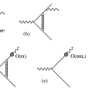
Figure 1: Parton level subprocesses contributing to the photon + 1 jet rate at ${\cal O}(\alpha\alpha_{s})$.

The parton level subprocesses contributing to the photon + 1 jet rate at ${\cal O}(\alpha\alpha_{s})$ are shown in Fig. 1.

• The tree level process $\gamma^{*}\to q\bar{q}g\gamma$, where the final state particles are clustered together such that a “photon jet” and one additional jet are observed in the final state. As the photon must be identified in the final state it cannot be soft.

• The one loop gluon correction to the $\gamma^{*}\to q\bar{q}\gamma$ process, where the photon and one of the quarks are clustered together or the photon is isolated while both quarks form a single jet.

• The process $\gamma^{*}\to q\bar{q}g$, where one of the quarks fragments into a photon while the remaining partons form only a single jet.

• The one loop gluon correction to the $\gamma^{*}\to q\bar{q}$ process, where one of the quarks fragments into a photon.

• The tree level process $\gamma^{*}\to q\bar{q}$ with a generic ${\cal O}(\alpha\alpha_{s})$ counterterm present in the bare quark-to-photon fragmentation function. Inclusion of this contribution absorbs all left over singularities of the processes cited above.

Each of these processes gives a singular contribution to the final photon + 1 jet rate. Therefore, to combine them together numerically in a way that can match onto the precise experimental cuts, we must first isolate the divergences analytically, so that the remaining finite contributions may be numerically evaluated. We choose to employ the hybrid subtraction method [28] which extends the phase space slicing method described in [15]. In this approach, we introduce a parton resolution parameter $y_{\rm min}$ to decide whether or not two partons are theoretically resolved; if, for example, $y_{ij}<y_{\rm min}$, then partons $i$ and $j$ are not resolved. In these unresolved regions, the matrix elements are singular, typically proportional to $1/y_{ij}$, and we analytically integrate approximate forms for the exact matrix elements over the restricted phase space. The essence of this approach can best be illustrated using the simple one-dimensional integral as suggested by Kunszt and Soper in [29],

$${\cal I}=\lim_{\epsilon\to 0}\left\{\int^{1}_{0}\frac{dx}{x}x^{\epsilon}F(x)-\frac{1}{\epsilon}F(0)\right\}.$$ (3.1)

$F(x)$ is a complicated function, which renders the evaluation of ${\cal I}$ analytically impossible. ${\cal I}$ could represent a $n$-jet cross section while $F(x)$ could stand for the $(n+1)$-parton bremsstrahlung matrix elements and $x$ for a scaled invariant mass $y_{ij}$. As $x\to 0$, which corresponds to the case when one of the final state particles becomes soft or collinear, the integrand is regularized by the $x^{\epsilon}$ factor as in dimensional regularization. The first term is however still divergent as $\epsilon\to 0$. This divergence is cancelled by the second term - which is the equivalent of the $n$-parton one-loop contribution - so that the integral is finite.

In the hybrid subtraction method [28], we choose to evaluate the integral by adding and subtracting the approximate matrix elements denoted by $F(0)$ in the unresolved regions of phase space, so that,

$${\cal I}\sim\lim_{\epsilon\to 0}\left\{\int^{1}_{0}\frac{dx}{x}x^{\epsilon}F(x)-F(0)\int^{y_{\rm min}}_{0}\frac{dx}{x}x^{\epsilon}+F(0)\int^{y_{\rm min}}_{0}\frac{dx}{x}x^{\epsilon}-\frac{1}{\epsilon}F(0)\right\}.$$

The approximate matrix elements are both simpler and process independent and the integrations over the unresolved phase space can be carried out analytically,

$$F(0)\int^{y_{\rm min}}_{0}\frac{dx}{x}x^{\epsilon}=\frac{1}{\epsilon}F(0)y_{\rm min}^{\epsilon},$$

so that,

$${\cal I} \sim \lim_{\epsilon\to 0}\left\{\int_{y_{\rm min}}^{1}\frac{dx}{x}x^{\epsilon}F(x)+\int_{0}^{y_{\rm min}}\frac{dx}{x}x^{\epsilon}\left[F(x)-F(0)\right]\right.$$ (3.2)

$$\left.+\frac{1}{\epsilon}F(0)y_{\rm min}^{\epsilon}-\frac{1}{\epsilon}F(0)\right\}$$

$$\sim \left\{\int_{y_{\rm min}}^{1}\frac{dx}{x}F(x)+\int_{0}^{y_{\rm min}}\frac{dx}{x}\left[F(x)-F(0)\right]+F(0)\ln(y_{\rm min})\right\}.$$

All three terms are now finite so that the $\epsilon\to 0$ limit may be safely taken and, furthermore, are in a form suitable for numerical evaluation.

Of course, the parton resolution parameter $y_{\rm min}$ is unphysical and the integral ${\cal I}$ or equivalently any physical process should not depend on $y_{\rm min}$. The $y_{\rm min}$ dependence of the three terms in eq. (3.2) should therefore cancel. In the evaluation of a jet cross section, this cancellation is usually realised numerically by a Monte Carlo program. This is not a straightforward point for the following reasons. The matrix element approximations used in the analytic part of the calculation are reliable only when $y_{\rm min}$ is small and are best when $y_{\rm min}$ is the smallest possible. On the other hand, smaller values of $y_{\rm min}$ generate larger cancellations amongst the terms, possibly giving rise to numerical instability problems. In practise $y_{\rm min}$ is chosen in such a way that the approximations performed in the analytic calculation are valid and that the numerical errors are minimized.

This approach, or the more basic phase space slicing method where the second term in eq. (3.2) is neglected, has been applied to a wide variety of processes; $e^{+}e^{-}\to 2~{}{\rm jets}$, $e^{+}e^{-}\to 3~{}{\rm jets}$ [15], $p\bar{p}\to W,Z+~{}1~{}{\rm jet}$, $p\bar{p}\to 2~{}{\rm jets}$  [30] and $ep\to e+~{}2~{}{\rm jets}$  [31]. In all of these next-to-leading order calculations, there can be at most one unresolved particle; one soft gluon or two collinear partons. In our calculation of the photon + 1 jet rate at ${\cal O}(\alpha\alpha_{s})$, we will be concerned, for the first time, with situations where two partons are unresolved.

So far we have described the various parton level processes contributing to the photon + 1 jet rate at ${\cal O}(\alpha\alpha_{s})$ and merely outlined the general structure of the contributions associated with these processes. Each of these processes contains different singular contributions that arise when one or more particles are theoretically unresolved. We now consider each process in turn, and use the parton resolution parameter $y_{\rm min}$ to define for each of them, the resolved and unresolved contributions from the resolved and unresolved regions of the phase space respectively. As we will see in sections 4-7, all theoretically unresolved contributions have the common structure already encountered in [15]. They can be written as the product of an unresolved factor containing all the singularities and a resolved cross section.

Note that in isolating the singularities, we are not concerned with the precise experimental jet definition. Provided the theoretical resolution parameter $y_{\rm min}$ is sufficiently small, any jet algorithm can be imposed numerically on the resolved parton cross sections, ${\rm d}\sigma^{R}$.

Figure 2: Different final state ‘photon’ + 1 jet topologies arising from the tree level $\gamma^{*}\to q\bar{q}\gamma g$ process. The ‘photon’ jet is moving to the left while the recoiling hadronic jet moves to the right. Square brackets denote theoretically unresolved particles, round brackets experimental clusters.

3.1 $\gamma^{*}\to q\bar{q}\gamma$ with real gluon bremsstrahlung

The various configurations where the tree level process $\gamma^{*}\to q\bar{q}g\gamma$ contributes to the photon + 1 jet rate are illustrated in Fig. 2. Note that topologies where the role of quark and antiquark are exchanged are also present, but are not shown. Jets formed when the experimental jet algorithm clusters particles together are denoted by $(ij)$, while theoretically unresolved clusters are denoted by $[ij]$. The associated real contributions can be separated into three categories: either theoretically resolved, single unresolved or double unresolved. Care must be taken to divide the phase space so that the different regions match onto each other. We must ensure that the difference of exact and approximate matrix elements tends to zero as the singularity is approached and equally, there is no overcounting of the singularities. This can be done by constraining the variables,

$$y_{q\gamma},~{}~{}~{}~{}~{}y_{\bar{q}\gamma},~{}~{}~{}~{}~{}y_{qg},~{}~{}~{}~{}~{}y_{\bar{q}g},$$

although in the double unresolved regions, we shall choose to constrain the combinations,

$$y_{q\gamma g},~{}~{}~{}~{}~{}~{}y_{\bar{q}\gamma g},$$

for certain configurations. The matrix elements contain poles in each of these six invariants, and are therefore singular as any of them tends to zero. There are two invariants, $y_{g\gamma}$ and $y_{q\bar{q}}$, which are not associated with any singularities and are therefore completely unconstrained.

The individual configurations can be structured as follows:

• Theoretically resolved contributions
  If all particles are resolved, a $\gamma$ + 1 jet event can only be formed if some final state particles are clustered together by the jet algorithm. The possible configurations yielding a photon + 1 jet event are displayed in Fig. 2.a. In principle this region is defined by requiring that all invariants are greater than the theoretical parton resolution parameter, $y_{\rm min}$, i.e. by requiring that,

  $$y_{q\gamma}>y_{\rm min},~{}~{}~{}~{}~{}y_{\bar{q}\gamma}>y_{\rm min},{}~{}~{}~{}~{}~{}y_{qg}>y_{\rm min},~{}~{}~{}~{}~{}y_{\bar{q}g}>y_{\rm min}.$$ (3.3)

  However, it turns out that the boundaries of this region are more subtle than that and must be chosen to match onto the boundaries of the unresolved regions. Consequently, the fully resolved region is defined as being the remaining phase space region of the four parton phase space when all unresolved regions are excluded.

• Single unresolved contributions
  As shown in Fig. 2.b, there are two classes of single (or one-particle) theoretically unresolved contributions, depending whether the gluon or the photon is unresolved. The single unresolved regions associated to these contributions are defined as follows:

  • The collinear quark-photon region
    If the photon is unresolved, it is collinear to the quark while the gluon is hard, i.e. the gluon is theoretically resolved but combined with the photon-quark cluster or with the antiquark by the experimental jet algorithm. Alternatively, the gluon forms a jet on its own while the antiquark is clustered into the photon jet. This can be defined by the constraints,

    $$y_{q\gamma}<y_{\rm min}\,y_{q\bar{q}\gamma},~{}~{}~{}~{}~{}y_{\bar{q}\gamma}>y_{\rm min}\,y_{q\bar{q}\gamma},{}~{}~{}~{}~{}~{}y_{q\gamma g}>y_{\rm min},~{}~{}~{}~{}~{}y_{\bar{q}g}>y_{\rm min},$$ (3.4)

    where $y_{q\bar{q}\gamma}$ is the scaled invariant mass of the radiating quark-antiquark-photon antenna, $s_{q\bar{q}\gamma}/M^{2}$.

  • The unresolved gluon region
    If the gluon is theoretically unresolved, it can be soft or collinear to the quark or to the antiquark, while the photon is experimentally combined with the quark to form the photon jet or is isolated while all other partons form a single jet. The three possible regions are defined by:

    • The collinear quark-gluon region

      $$y_{qg}<y_{\rm min}\,y_{q\bar{q}g},~{}~{}~{}~{}~{}y_{\bar{q}g}>y_{\rm min}\,y_{q\bar{q}g},{}~{}~{}~{}~{}~{}y_{q\gamma g}>y_{\rm min},~{}~{}~{}~{}~{}y_{\bar{q}\gamma}>y_{\rm min},$$ (3.5)

    • The collinear antiquark-gluon region

      $$y_{\bar{q}g}<y_{\rm min}\,y_{q\bar{q}g},~{}~{}~{}~{}~{}y_{qg}>y_{\rm min}\,y_{q\bar{q}g},{}~{}~{}~{}~{}~{}y_{q\gamma g}>y_{\rm min},~{}~{}~{}~{}~{}y_{\bar{q}\gamma}>y_{\rm min},$$ (3.6)

    • The soft gluon region

      $$y_{qg}<y_{\rm min}\,y_{q\bar{q}g},~{}~{}~{}~{}~{}y_{\bar{q}g}<y_{\rm min}\,y_{q\bar{q}g},{}~{}~{}~{}~{}~{}y_{q\gamma}>y_{\rm min},~{}~{}~{}~{}~{}y_{\bar{q}\gamma}>y_{\rm min}.$$ (3.7)

    As in the unresolved photon case, the mass of the antenna radiating the gluon, $y_{q\bar{q}g}$ plays a role in determining when the approximate matrix elements are used.

• Double unresolved contributions
  These contributions arise when both the photon and the gluon are theoretically “unseen” in the final state. As the photon has to be seen in the final state, it can only be collinear with the quark and cannot be soft. The gluon on the other hand can be collinear with the quark or with the antiquark or it can be soft. Corresponding to these different final state configurations we define three double unresolved phase space regions:

  • The triple collinear region
    The photon and the gluon are simultaneously collinear with the quark. Here we need to constrain the “triple” invariant $y_{q\gamma g}\equiv y_{q\gamma}+y_{qg}+y_{\gamma g}$ since it appears in the denominator of the four-particle matrix elements,

    $$y_{q\gamma g}<y_{\rm min}\hskip 14.22636pt{\rm and}\hskip 14.22636pty_{\bar{q}g}>y_{\rm min}.$$ (3.8)

    Note that this implies $y_{q\gamma}<y_{\rm min}$ and $y_{qg}<y_{\rm min}$. We require $y_{\bar{q}g}>y_{\rm min}$ since in this region the gluon is collinear but not soft.

  • The soft/collinear region
    The photon is collinear with the quark while the gluon is soft,

    $$y_{q\gamma}<y_{\rm min}\hskip 14.22636pt{\rm and}\hskip 14.22636pty_{qg}<y_{\rm min}\hskip 14.22636pt{\rm and}\hskip 14.22636pty_{\bar{q}g}<y_{\rm min}.$$ (3.9)

  • The double single collinear region
    The photon is collinear with the quark while the gluon is collinear with the antiquark,

    $$y_{q\gamma}<y_{\rm min}\hskip 14.22636pt{\rm and}\hskip 14.22636pty_{qg}>y_{\rm min}\hskip 14.22636pt{\rm and}\hskip 14.22636pty_{\bar{q}g}<y_{\rm min}.$$ (3.10)

  For these three contributions, the final state configuration corresponds already to a photon +1 jet event. Hence, the final state particles will not be clustered further by the jet algorithm. These contributions are schematically displayed in Fig. 2.c. As before, these regions are matched by three analogous double unresolved regions where the photon clusters with the antiquark.

The decomposition of the four-particle phase space is summarized in Fig. 3. In this table, we have specified which invariants are less than $y_{\rm min}$ (or a cut proportional to $y_{\rm min}$) for each singular region of phase space. We have also noted which invariants are greater than $y_{\rm min}$ to eliminate overlaps between regions determined by the same combinations of invariants less than $y_{\rm min}$. Invariants that are not specified are completely unconstrained.

Figure 3: Phase space decomposition of the real $\gamma^{\star}\to q\bar{q}\gamma g$ contributions. Note that the single and double unresolved regions where the photon clusters with the antiquark are not shown. For these regions, the necessary cuts are obtained by exchanging $q$ and $\bar{q}$. Altogether, there are five single unresolved and six double unresolved regions.

3.2 $\gamma^{*}\to q\bar{q}\gamma$ with a virtual gluon

The final state topology is similar to that for the lowest order $\gamma^{*}\to q\bar{q}\gamma$ contribution discussed in [4] and contributes to the photon + 1 jet rate, if two of the final state partons are clustered together. We distinguish the theoretically unresolved collinear quark-photon contribution from the contributions where the theoretically resolved photon is clustered with the quark by the experimental jet algorithm to form the photon jet or isolated while quark and antiquark combine to form the jet. The three particle phase space therefore divides as follows:

• The resolved photon region
  

  $$y_{q\gamma}>y_{\rm min},~{}~{}~{}~{}~{}y_{\bar{q}\gamma}>y_{\rm min}.$$ (3.11)

• The quark-photon collinear region
  

  $$y_{q\gamma}<y_{\rm min},~{}~{}~{}~{}~{}y_{\bar{q}\gamma}>y_{\rm min},$$ (3.12)

  plus a similar region for the collinear antiquark-photon configuration.

3.3 $\gamma^{*}\to q\bar{q}(g)$ with fragmentation

The ${\cal O}(\alpha_{s})$ processes with associated fragmentation shown in Fig. 1.c and 1.d contribute to the photon + 1 jet cross section if, in addition to the photon-jet, only a single jet is formed. As illustrated in Fig. 4, the gluon may be resolved, unresolved or virtual, while the photon is produced via the fragmentation process. There are five distinct contributions:

• The resolved gluon region
  The real gluon is theoretically resolved, but may be clustered by the experimental jet algorithm with either the photon fragmentation cluster or with the antiquark or it may form a jet on its own, while the antiquark is combined with the photon/quark cluster.

  $$y_{qg}>y_{\rm min},~{}~{}~{}~{}~{}y_{\bar{q}g}>y_{\rm min}.$$ (3.13)

• The unresolved gluon region
  If the gluon is theoretically unresolved, it can be soft or collinear to the fragmenting quark or to the antiquark. The three possible regions are defined by:

  • The collinear quark-gluon region
    

    $$y_{qg}<y_{\rm min},~{}~{}~{}~{}~{}y_{\bar{q}g}>y_{\rm min}.$$ (3.14)

  • The collinear antiquark-gluon region
    

    $$y_{qg}>y_{\rm min},~{}~{}~{}~{}~{}y_{\bar{q}g}<y_{\rm min}.$$ (3.15)

  • The soft gluon region
    

    $$y_{qg}<y_{\rm min},~{}~{}~{}~{}~{}y_{\bar{q}g}<y_{\rm min}.$$ (3.16)

• The gluon is virtual.

Since this process is already of ${\cal O}(\alpha_{s})$, only the ${\cal O}(\alpha)$ counterterm in the bare fragmentation function contributes.

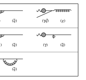
Figure 4: Different final state ‘photon’ + 1 jet topologies arising from the $\gamma^{*}\to q\bar{q}(g)$ process with subsequent fragmentation of the quark into a photon. The ‘photon’ jet is moving to the left while the recoiling hadronic jet moves to the right. Square brackets denote theoretically unresolved particles, round brackets represent experimental clusters.

3.4 $\gamma^{*}\to q\bar{q}$ with fragmentation

In addition to the processes described above involving a real or virtual gluon, one has to consider a contribution to the photon + 1 jet rate from the generic ${\cal O}(\alpha\alpha_{s})$ counterterm present in the bare fragmentation function of eq. (LABEL:eq:counter).

4 Resolved and Single unresolved contributions

In the next two sections, we will discuss the contributions to the $\gamma$ + 1 jet rate at ${\cal O}(\alpha\alpha_{s})$ relevant to the process $\gamma^{*}\to q\bar{q}\gamma$ with real gluon bremsstrahlung. As shown in Fig. 2, there are many different topologies contributing which can be divided according to the number of theoretically unresolved particles. In this section, we consider the cases where at most one particle is unresolved, while the double unresolved contributions are studied in section 5.

The $\gamma^{*}\to q\bar{q}\gamma g$ process contributes to the $\gamma$ + 1 jet differential cross section if the final state configuration is such that only the photon jet and a single associated jet are observed. The generic contribution of this four particle final state process to the rate can be written as,

$${\rm d}\sigma_{q\bar{q}\gamma g}=\left(\frac{\alpha_{s}C_{F}}{2\pi}\right)\left(\frac{\alpha e_{q}^{2}}{2\pi}\right)\mu^{4\epsilon}4(2\pi)^{4}\frac{1}{2M^{2}}\int|{\cal M}_{q\bar{q}\gamma g}|^{2}{\rm d}P_{4}^{(d)}(M;p_{q},p_{\bar{q}},p_{\gamma},p_{g}).$$ (4.1)

Here $|{\cal M}_{q\bar{q}\gamma g}|^{2}$ represents the squared matrix elements in $d$-dimensions, while the Lorentz invariant phase space for the decay of an off-shell photon with $p_{\gamma^{*}}^{2}=M^{2}$ can be written,

$$\int{\rm d}P_{4}^{(d)}(M;p_{q},p_{\gamma},p_{g},p_{\bar{q}}) = \frac{M^{4-6\epsilon}}{2^{7-4\epsilon}(2\pi)^{8-6\epsilon}}\int{\rm d}\Omega_{d-1}\;{\rm d}\Omega_{d-2}\;{\rm d}\Omega_{d-3}{\rm d}y_{q\bar{q}}\;{\rm d}y_{q\gamma}{\rm d}y_{qg}{\rm d}y_{\bar{q}\gamma}{\rm d}y_{\bar{q}g}{\rm d}y_{\gamma g}$$ (4.2)

$$\times {(-\Delta_{4})}^{-1/2-\epsilon}\;\delta(y_{q\bar{q}}+y_{q\gamma}+y_{qg}+y_{\bar{q}\gamma}+y_{\bar{q}g}+y_{\gamma g}-1),$$

with,

$$\Delta_{4}={y_{q\bar{q}}}^{2}{y_{\gamma g}}^{2}\;+\;{y_{q\gamma}}^{2}{y_{\bar{q}g}}^{2}\;+\;{y_{qg}}^{2}{y_{\bar{q}\gamma}}^{2}-2\bigg{(}y_{q\bar{q}}y_{\bar{q}\gamma}y_{\gamma g}y_{qg}\;+\;y_{q\gamma}y_{\bar{q}\gamma}y_{\bar{q}g}y_{qg}\;+\;y_{q\bar{q}}y_{\bar{q}g}y_{\gamma g}y_{q\gamma}\bigg{)}.$$ (4.3)

The matrix elements are well known and contain terms up to ${\cal O}(\epsilon^{3})$. These additional contributions, which vanish in 4-dimensions, are important in determining the contributions from the unresolved regions which may contain singularities up to ${\cal O}(1/\epsilon^{3})$.

4.1 The resolved contributions

In the resolved phase space region which is the region of the four-particle phase space left over when all unresolved regions specified in Fig. 3 are excluded, the matrix element squared is finite. Thus we may take the $\epsilon\to 0$ limit for both matrix elements and phase space, so that

$${\rm d}\sigma^{(R)}_{q\bar{q}\gamma g}=\left(\frac{\alpha_{s}C_{F}}{2\pi}\right)\left(\frac{\alpha e_{q}^{2}}{2\pi}\right)4(2\pi)^{4}\frac{1}{2M^{2}}\int|{\cal M}_{q\bar{q}\gamma g}|^{2}{\rm d}P_{4}^{(R)}(M;p_{q},p_{\bar{q}},p_{\gamma},p_{g}),$$ (4.4)

where the phase space ${\rm d}P_{4}^{(R)}$ is restricted to this resolved region. For these resolved contribution, the integration is carried out numerically and the photon and jet definitions applied directly to the final state particles. As we are employing the hybrid subtraction method to calculate the photon +1 jet cross section, there are additional contributions which are to be numerically calculated. Those come from evaluating the difference between the exact and approximate squared matrix elements in the various unresolved regions of phase space.

4.2 The single unresolved contributions

There are two classes of single unresolved real contributions depending on whether the photon or the gluon is unresolved. If the photon is unresolved, it is collinear to the quark while if the gluon is unresolved it can be collinear to the quark, collinear to the antiquark or it can be soft. The possible final state configurations of single unresolved contributions yielding a $\gamma$ +1 jet event are displayed in Fig. 2.(b). In each unresolved region of the four-particle phase space we expect to be able to write the differential cross section as the product of a one particle unresolved factor and a three-particle cross section [15].

4.2.1 The unresolved gluon contribution

The phase space region where the quark and the gluon are collinear is defined by eq. (3.5),

$$y_{qg}<y_{\rm min}\,y_{q\bar{q}g},~{}~{}~{}~{}~{}y_{\bar{q}g}>y_{\rm min}\,y_{q\bar{q}g},{}~{}~{}~{}~{}~{}y_{q\gamma g}>y_{\rm min},~{}~{}~{}~{}~{}y_{\bar{q}\gamma}>y_{\rm min}.$$

Here, the quark and the gluon cluster to form a new parton $Q$ such that,

$$p_{q}+p_{g}=p_{Q},$$

and carry respectively a fraction $y$ and $1-y$ of the parent parton momentum $p_{Q}$. The fractional momentum $y$ is defined with respect to the momenta carried by the colour connected particles: the quark, the antiquark and the gluon. In particular $y$ is defined as,

$$y\equiv\frac{y_{\bar{q}g}}{y_{q\bar{q}g}},$$ (4.5)

and, since $y_{\bar{q}g}>y_{\rm min}y_{q\bar{q}g}$, the lower boundary of the $y$ integral is $y_{\rm min}$. In this limit the four particle invariants are related to the invariants of the three remaining particles,

$$y_{q\bar{q}}=(1-y)\,y_{Q\bar{q}},\hskip 28.45274pty_{\bar{q}g}=y\,y_{Q\bar{q}},\hskip 28.45274pty_{q\bar{q}g}=y_{Q\bar{q}}$$ (4.6)

while the invariants containing $p_{\gamma}$ become,

$$y_{q\gamma}=(1-y)\,y_{Q\gamma},\hskip 28.45274pty_{\gamma g}=y\,y_{Q\gamma}.$$

The matrix elements and phase space exhibit an overall factorization,

$$|{\cal M}_{q\bar{q}\gamma g}|^{2}\to P_{qg\to Q}(y,s_{qg})|{\cal M}_{Q\bar{q}\gamma}|^{2},$$ (4.7)

with, $|{\cal M}_{Q\bar{q}\gamma}|^{2}$ the three-particle matrix element squared for the scattering of a quark-antiquark pair with a photon, and,

$$P_{qg\to Q}(y,s_{qg})=\frac{2}{s_{qg}}P_{q\to g}(y).$$ (4.8)

Similarly, the four particle phase space becomes,

$${\rm d}P_{4}^{(d)}(M;p_{q},p_{\bar{q}},p_{\gamma},p_{g})\to{\rm d}P_{3}^{(d)}(M;p_{Q},p_{\bar{q}},p_{\gamma})\,{\rm d}P^{(d)}_{col}(p_{q},p_{g},y)$$ (4.9)

where ${\rm d}P_{3}^{(d)}(M;p_{Q},p_{\bar{q}},p_{\gamma})$ is the three-particle Lorentz invariant phase space in $d$-dimensions. The collinear phase space factor reads [15],

$${\rm d}P^{(d)}_{col}(p_{q},p_{g},y)=\frac{(4\pi)^{\epsilon}}{16\pi^{2}\Gamma(1-\epsilon)}{\rm d}s_{qg}\,{\rm d}y\,s_{qg}^{-\epsilon}y^{-\epsilon}(1-y)^{-\epsilon}.$$ (4.10)

To evaluate the quark-gluon collinear factor, we need to integrate the collinear matrix element squared over the unresolved variables $y_{qg}$ and $y$. Reinserting the overall coupling factor, we have,

$$\tilde{C}_{F}(q) = \int g_{s}^{2}C_{F}\mu^{2\epsilon}P_{qg\to Q}(y,s_{qg}){\rm d}P^{(d)}_{col}(p_{q},p_{g},y)$$

$$= \left(\frac{\alpha_{s}C_{F}}{2\pi}\right)\left(\frac{4\pi\mu^{2}}{M^{2}}\right)^{\epsilon}\frac{2}{\Gamma(1-\epsilon)}\int_{0}^{y_{\rm min}y_{q\bar{q}g}}{\rm d}y_{qg}\,y_{qg}^{-\epsilon-1}\int_{y_{\rm min}}^{1}{\rm d}yy^{-\epsilon}(1-y)^{-\epsilon}P_{q\to g}(y)$$

$$= -\frac{1}{\epsilon}\left(\frac{\alpha_{s}C_{F}}{2\pi}\right)\left(\frac{4\pi\mu^{2}}{M^{2}}\right)^{\epsilon}\frac{1}{\Gamma(1-\epsilon)}y_{\rm min}^{-\epsilon}y_{Q\bar{q}}^{-\epsilon}\left[\frac{2}{\epsilon}y_{\rm min}^{-\epsilon}\;-\;\frac{(1-\epsilon)(4-\epsilon)}{2\epsilon(1-2\epsilon)}\;\frac{\Gamma^{2}(1-\epsilon)}{\Gamma(1-2\epsilon)}\;\right].$$

We see that compared to the single quark-gluon collinear factor obtained considering the single quark-gluon collinear limit of a three parton cross section found in [15], the collinear factor given by eq. (LABEL:eq:cfq) is multiplied by $y_{Q\bar{q}}^{-\epsilon}$. This slight modification is caused by the change in the boundary of the $y_{qg}$ integration. The invariant $y_{qg}$ is here bounded to be less than $y_{\rm min}y_{q\bar{q}g}$ instead of $y_{\rm min}$ in the three parton case.

Putting all the factors together, we find that in the collinear $quark-gluon$ limit the four particle differential cross section ${\rm d}\sigma_{4}$ becomes,

$${\rm d}\sigma_{4}\to\tilde{C}_{F}(q)\times\left(\frac{\alpha e_{q}^{2}}{2\pi}\right)2(2\pi)^{2}\frac{1}{2M^{2}}\int|{\cal M}_{Q\bar{q}\gamma}|^{2}{\rm d}P_{3}^{(d)}(M;p_{Q},p_{\bar{q}},p_{\gamma})=\tilde{C}_{F}(q)\times{\rm d}\sigma_{Q\bar{q}\gamma},$$ (4.12)

where ${\rm d}\sigma_{Q\bar{q}\gamma}$ is the three-particle differential cross section for the scattering of a quark-antiquark with an additional hard photon. All of the divergences are isolated in $\tilde{C}_{F}(q)$ and therefore ${\rm d}\sigma_{Q\bar{q}\gamma}$ can be evaluated in 4-dimensions.

In the region where the antiquark and the gluon are collinear the roles of quark and antiquark are exchanged. Now, the antiquark and gluon form a parent parton $\bar{Q}$ and the resulting contribution in this region of the four particle phase space therefore yields,

$${\rm d}\sigma_{q\bar{q}\gamma g}\to\tilde{C}_{F}(\bar{q})\;{\rm d}\sigma_{q\bar{Q}\gamma},$$ (4.13)

where, since $y_{Q\bar{q}}\equiv y_{q\bar{Q}}$,

$$\tilde{C}_{F}(\bar{q})=\tilde{C}_{F}(q).$$ (4.14)

In order to match onto the single collinear quark-gluon regions, the soft gluon region is defined in eq. (3.7),

$$y_{qg}<y_{\rm min}\,y_{q\bar{q}g},~{}~{}~{}~{}~{}y_{\bar{q}g}<y_{\rm min}\,y_{q\bar{q}g},{}~{}~{}~{}~{}~{}y_{q\gamma}>y_{\rm min},~{}~{}~{}~{}~{}y_{\bar{q}\gamma}>y_{\rm min}.$$

As in the collinear regions, the matrix elements and phase space both factorise in the soft gluon limit,

$$|{\cal M}_{q\bar{q}\gamma g}|^{2}\to|{\cal M}_{q\bar{q}\gamma}|^{2}\,f_{q\bar{q}}(g),$$ (4.15)

with the eikonal factor,

$$f_{q\bar{q}}(g)=\frac{4s_{q\bar{q}}}{s_{qg}s_{\bar{q}g}},$$

and,

$${\rm d}P_{4}^{(d)}(M;p_{q},p_{\bar{q}},p_{\gamma},p_{g})\to{\rm d}P_{3}^{(d)}(M;p_{q},p_{\bar{q}},p_{\gamma})\,{\rm d}P^{(d)}_{soft}(p_{q},p_{\bar{q}},p_{g}),$$ (4.16)

where the soft phase space factor reads [15],

$${\rm d}P^{(d)}_{soft}(p_{q},p_{\bar{q}},p_{g})=\frac{(4\pi)^{\epsilon}}{16\pi^{2}\Gamma(1-\epsilon)}\frac{{\rm d}s_{qg}{\rm d}s_{\bar{q}g}}{s_{q\bar{q}}}\left[\frac{s_{qg}s_{\bar{q}g}}{s_{q\bar{q}}}\right]^{-\epsilon}.$$

As before, all of the dependence on the unresolved variables is collected into the soft approximations to the matrix elements and the phase space. We find,

$$\tilde{S}_{F} = \int g_{s}^{2}C_{F}\mu^{2\epsilon}f_{q\bar{q}}(g){\rm d}P^{(d)}_{soft}(p_{q},p_{\bar{q}},p_{g})$$ (4.17)

$$= \left(\frac{\alpha_{s}C_{F}}{2\pi}\right)\left(\frac{4\pi\mu^{2}}{M^{2}}\right)^{\epsilon}\frac{1}{\Gamma(1-\epsilon)}\,\frac{2}{y_{q\bar{q}}}\int_{0}^{y_{\rm min}y_{q\bar{q}}}{\rm d}y_{qg}\int_{0}^{y_{\rm min}y_{q\bar{q}}}{\rm d}y_{\bar{q}g}\,\;\left[\frac{y_{qg}y_{\bar{q}g}}{y_{q\bar{q}}}\right]^{-\epsilon-1}$$

$$= \left(\frac{\alpha_{s}C_{F}}{2\pi}\right)\left(\frac{4\pi\mu^{2}}{M^{2}}\right)^{\epsilon}\frac{1}{\Gamma(1-\epsilon)}\,\frac{2}{\epsilon^{2}}\;\,y_{\rm min}^{-2\epsilon}y_{q\bar{q}}^{-\epsilon}.$$

Again, apart from the changed boundaries, this is the same soft factor as given in eq. (3.33) of [15]. As usual, the contribution to the cross section from the single soft singular region factorizes,

$${\rm d}\sigma_{q\bar{q}\gamma g}\to\tilde{S}_{F}\;{\rm d}\sigma_{q\bar{q}\gamma}.$$ (4.18)

The sum of the single unresolved gluon contributions is then given by combining eqs. (4.12), (4.13) and (4.18),

$${\rm d}\sigma_{q\bar{q}\gamma g}\to\left(\tilde{C}_{F}(q)+\tilde{C}_{F}(\bar{q})+\tilde{S}_{F}\right){\rm d}\sigma_{q\bar{q}\gamma}\equiv{R_{q\bar{q}\gamma}}{\rm d}\sigma_{q\bar{q}\gamma},$$

where the real unresolved factor $R_{q\bar{q}\gamma}$ depends on the invariant mass of the quark-antiquark pair and is given by,

$${R_{q\bar{q}\gamma}} = \left(\frac{\alpha_{s}C_{F}}{2\pi}\right)\frac{1}{\Gamma(1-\epsilon)}\left(\frac{4\pi\mu^{2}}{M^{2}}\right)^{\epsilon}$$ (4.19)

$$\times\left(\frac{2\;y_{q\bar{q}}^{-\epsilon}}{\epsilon^{2}}+\frac{3}{\epsilon}-2\ln^{2}(y_{\rm min})-3\ln(y_{q\bar{q}}\;y_{\rm min})+7-\frac{2\pi^{2}}{3}\right).$$

This is the same real unresolved factor as defined in eq. (3.79) of [15] with $y_{\rm min}\to y_{\rm min}y_{q\bar{q}}$ reflecting the changed boundaries of the unresolved gluon region of the four parton phase space compared with the unresolved gluon region of the three parton phase space. The singularities present in these single unresolved gluon contributions will cancel with those from the resolved photon one-loop $\gamma^{*}\to q\bar{q}\gamma$ process discussed in section 6.1.

4.2.2 The unresolved photon contribution

In the region where the quark and the photon are collinear we have, cf. eq. (3.4),

$$y_{q\gamma}<y_{\rm min}\,y_{q\bar{q}\gamma},~{}~{}~{}~{}~{}y_{\bar{q}\gamma}>y_{\rm min}\,y_{q\bar{q}\gamma},{}~{}~{}~{}~{}~{}y_{q\gamma g}>y_{\rm min},~{}~{}~{}~{}~{}y_{\bar{q}g}>y_{\rm min}.$$ (4.20)

The quark and the photon cluster to form a new parent parton $Q$ such that each carries respectively a fraction $z$ and $1-z$ of the parent parton momentum $p_{Q}$. The four-particle matrix elements and phase space factorize in exactly the same way as in the quark-gluon collinear limit with the roles of photon and gluon being interchanged and $y$ replaced by $z$. Unlike the quark-gluon case however, the photon is observed in the final state and hence only $y_{q\gamma}$ is an unresolved variable. The momentum fraction $z$ carried by the photon inside the quark-photon cluster is defined with respect to the momenta carried by the electromagnetically connected particles,

$$z=\frac{y_{\bar{q}\gamma}}{y_{q\bar{q}\gamma}}.$$ (4.21)

In this limit, the four particle differential cross section again factorizes,

$${\rm d}\sigma_{4}\to\tilde{C}_{F\gamma}(q){\rm d}z\times{\rm d}\sigma_{Q\bar{q}g}$$ (4.22)

where ${\rm d}\sigma_{Q\bar{q}g}$ is the differential cross section for the production of a quark-antiquark pair and a gluon. The singular factor $\tilde{C}_{F\gamma}(q)$ is,

$$\tilde{C}_{F\gamma}(q)=-\left(\frac{\alpha e_{q}^{2}}{2\pi}\right)\left(\frac{4\pi\mu^{2}}{M^{2}}\right)^{\epsilon}\frac{1}{\Gamma(1-\epsilon)}\frac{2}{\epsilon}\;y_{\rm min}^{-\epsilon}\;y_{Q\bar{q}}^{-\epsilon}\;z^{-\epsilon}\;(1-z)^{-\epsilon}\;P_{q\to\gamma}(z).$$ (4.23)

There is a similar contribution where the photon is collinear with the antiquark.

4.2.3 Overlapping of single collinear regions

It is worth noting that in both, $q-g$ and $q-\gamma$ collinear regions we have required $y_{q\gamma g}>y_{\rm min}$ in order to guarantee that these regions match onto the double unresolved triple collinear region defined by $y_{q\gamma g}<y_{\rm min}$. However this requirement has an important consequence. We do not avoid the situation where both invariants $y_{q\gamma}$ and $y_{qg}$ are simultaneously less than $y_{\rm min}$ and the constraints,

$$y_{q\gamma}<y_{\rm min}\hskip 28.45274pty_{qg}<y_{\rm min}\hskip 28.45274pt{\rm but}\hskip 28.45274pty_{q\gamma g}>y_{\rm min},$$ (4.24)

define an overlapping region of the two single collinear $q-\gamma$ and $q-g$ regions. In this overlapping region, the matrix elements are correctly approximated by the sum of the two single collinear approximations and the error in the analytic contribution resulting from evaluating the approximated matrix elements over this restricted phase space region is of ${\cal O}(y_{\rm min})$ and therefore negligible.

However, as we mentioned before, the photon + 1 jet rate is to be evaluated numerically applying the hybrid subtraction method. It is then crucial to ensure that the matrix elements are correctly approximated in this overlapping region since here we evaluate the difference between this approximation given by the sum of both collinear approximations and the full matrix elements. It is precisely to take into account these numerical contributions (which generate terms proportional to $\ln(y_{\rm min})$) that we are constrained to apply the hybrid subtraction scheme rather then the more commonly used phase space slicing method [14, 15] where the two single collinear regions would have to be clearly distinct and not overlapping. However, in this region of phase space, either collinear limit on its own is a very poor approximation to the full matrix elements. As a consequence, using the phase space slicing approach, we would fail to obtain the necessary $\ln(y_{\rm min})$ cancellation in the physical photon + 1 jet cross section.

5 Double unresolved contributions

In the previous section we have discussed the resolved and single unresolved real contributions relevant to the tree level process $\gamma^{*}\to q\bar{q}\gamma g$. Each of these two classes of real contributions corresponds to final state configurations where more than two particles are theoretically “seen” and a $\gamma$ + 1 jet event can only arise if some final state particles are clustered together by the jet algorithm. Therefore, to allow the adjustment of our results to any jet algorithm used in the experimental analysis, the finite contributions to the differential cross section will be evaluated numerically. The two-particle unresolved contributions, on the other hand, already correspond to $\gamma$ + 1 jet events, and there is no further clustering by the jet algorithm needed. Because of this, the integrations can be performed analytically.

5.1 The triple collinear factor

As we saw in section 3, the triple collinear contributions arise when the gluon and the photon are collinear to the quark. The triple collinear configuration is illustrated in Fig. 2.c.i. In order to evaluate these contributions we need to determine the appropriate approximations for the matrix element squared and phase space in the triple collinear limit and perform the phase space integrals over the unresolved variables.

The triple collinear region of phase space is defined by eq. (3.8),

$$y_{q\gamma g}<y_{\rm min}\hskip 14.22636pt{\rm and}\hskip 14.22636pty_{\bar{q}g}>y_{\rm min}.$$

In this limit, $y_{qg\gamma}$ is small and the photon, gluon and quark cluster to form a new parent parton Q such that,

$$p_{q}+p_{\gamma}+p_{g}=p_{Q}.$$ (5.1)

The photon, the gluon and the quark carry respectively a fraction $z$, $y$ and $(1-y-z)$ of the parent parton momentum $p_{Q}$,

$$p_{\gamma}=z~{}p_{Q},\hskip 28.45274ptp_{g}=y~{}p_{Q},\hskip 28.45274ptp_{q}=(1-z-y)~{}p_{Q},$$ (5.2)

so that the invariants are given by the following,

$$y_{q\bar{q}} = (1-y-z)\,y_{Q\bar{q}}\equiv(1-y-z),$$

$$y_{\bar{q}\gamma} = z\,y_{Q\bar{q}}\equiv z,$$ (5.3)

$$y_{\bar{q}g} = y\,y_{Q\bar{q}}\equiv y.$$

The algebraic structure of these double unresolved contributions is unique to the triple collinear limit of the matrix element squared, and when analytically integrated over the singular regions of phase space will form the triple collinear factor. These contributions are expected to arise in analytic calculations of exclusive quantities at the second order in perturbation theory. Such calculations have, to the best of our knowledge, not been performed before in the literature.

We are interested in the triple collinear limit of the matrix element squared for the scattering of a quark-antiquark pair with a photon and a gluon. In this limit the $d$-dimensional four-particle matrix element squared factorises,

$$|{\cal M}_{q\bar{q}g\gamma}|^{2}\to P_{qg\gamma\to Q}(z,y,s_{q\gamma},s_{qg},s_{qg\gamma})|{\cal M}_{Q\bar{q}}|^{2},$$

where $|{\cal M}_{Q\bar{q}}|^{2}$ is the two-particle matrix element squared and $P_{qg\gamma\to Q}(z,y,s_{q\gamma},s_{qg},s_{qg\gamma})$ defines the triple collinear splitting function. It is obtained by keeping only the terms containing a pair of the unresolved invariants, $s_{q\gamma}$, $s_{qg}$ and $s_{qg\gamma}$, in the denominator of the “full” four particle squared matrix elements $|{\cal M}_{q\bar{q}g\gamma}|^{2}$,

$$P_{qg\gamma\to Q}(z,y,s_{q\gamma},s_{qg},s_{qg\gamma})=$$ (5.4)

$$+ \frac{4}{s_{q\gamma}s_{qg}}\frac{(1-z-y)(1+(1-z-y)^{2}-\epsilon(z^{2}+zy+y^{2})-\epsilon^{2}zy)}{zy}$$

$$+ \frac{4}{s_{q\gamma}s_{qg\gamma}}\frac{(1-z-y)(1-z+\epsilon^{2}zy)+(1-y)^{3}-\epsilon(1-y)(z^{2}+zy+y^{2})+\epsilon^{2}zy}{zy}$$

$$+ \frac{4}{s_{qg}s_{qg\gamma}}\frac{(1-z-y)(1-y+\epsilon^{2}zy)+(1-z)^{3}-\epsilon(1-z)(z^{2}+zy+y^{2})+\epsilon^{2}zy}{zy}$$

$$- \frac{4(1-\epsilon)}{s_{qg\gamma}^{2}}\left((1-\epsilon)\frac{s_{q\gamma}}{s_{qg}}+(1-\epsilon)\frac{s_{qg}}{s_{q\gamma}}-2\epsilon\right).$$

This triple collinear splitting function is the generalization of the single collinear factor with three collinear particles instead of two and is as universal as the single soft and single collinear factors encountered earlier in section 4.

In the triple collinear limit, we can reorganise the $d$-dimensional four particle phase space given in eq. (4.2) into one part appropriate for the remnant $Q-\bar{q}$ pair multiplied by the integral over all of the unresolved variables,

$${\rm d}P_{4}^{(d)}(M;p_{q},p_{\gamma},p_{g},p_{\bar{q}})\;\to\;{\rm d}P_{2}^{(d)}(M;p_{Q},p_{\bar{q}})\times{\rm d}P_{tricol}^{(d)}(p_{Q},p_{q},p_{\gamma},p_{g}),$$

where ${\rm d}P_{2}^{(d)}(M;p_{Q},p_{\bar{q}})$ is the usual two body phase space and,

$${\rm d}P_{tricol}^{(d)}(p_{Q},p_{q},p_{\gamma},p_{g}) = \frac{1}{\Gamma(1-2\epsilon)}\frac{1}{4\pi}\frac{M^{4}}{4(2\pi)^{4}}\left(\frac{4\pi}{M^{2}}\right)^{2\epsilon}\left[-\Delta_{4}\right]^{-\frac{1}{2}-\epsilon}$$ (5.5)

$$\times {\rm d}y_{q\gamma g}\;{\rm d}y_{q\gamma}\;{\rm d}y_{qg}\;{\rm d}y_{\gamma g}\;{\rm d}z\;{\rm d}y\;\delta(y_{q\gamma}+y_{qg}+y_{\gamma g}-y_{q\gamma g}).$$

Here the angular integrations for the rotation of the $qg\gamma$-system around the $\bar{q}$ axis and for the parity of the $qg\gamma$-system have been performed. In terms of the unresolved variables, the Gram determinant is,

$$\Delta_{4}\to\big{(}(1-y-z)\;y_{\gamma g}\;-\;y\;y_{q\gamma}\;-\;z\;y_{qg}\big{)}^{2}-4zy\;y_{q\gamma}\;y_{qg}.$$

Reinserting all coupling factors into the matrix elements, we find that in the triple collinear limit, the cross section factorises,

$${\rm d}\sigma_{4} \equiv \left(\frac{\alpha_{s}C_{F}}{2\pi}\right)\left(\frac{\alpha e_{q}^{2}}{2\pi}\right)4(2\pi)^{4}\mu^{4\epsilon}\;\int|{\cal M}_{q\bar{q}g\gamma}|^{2}\;{\rm d}P_{4}^{(d)}(M;p_{q},p_{\bar{q}},p_{\gamma},p_{g})$$ (5.6)

$$\to TC_{F\gamma}{\rm d}z\times\int|{\cal M}_{Q\bar{q}}|^{2}{\rm d}P_{2}^{(d)}(M;p_{Q},p_{\bar{q}})$$

$$\equiv TC_{F\gamma}{\rm d}z\times\sigma_{0}.$$

As usual, $\sigma_{0}$ is the two-particle cross section while the dimensionless factor $TC_{F\gamma}{\rm d}z$ containing all the singularities is formally given by,

$$TC_{F\gamma}{\rm d}z \equiv \left(\frac{\alpha_{s}C_{F}}{2\pi}\right)\left(\frac{\alpha e_{q}^{2}}{2\pi}\right)\left(\frac{4\pi\mu^{2}}{M^{2}}\right)^{2\epsilon}\frac{1}{\Gamma(1-2\epsilon)}\frac{1}{4\pi}$$ (5.7)

$$\times \int\left[-\Delta_{4}\right]^{-\frac{1}{2}-\epsilon}P_{qg\gamma\to Q}(z,y,y_{q\gamma},y_{qg},y_{qg\gamma})$$

$$\times{\rm d}y_{q\gamma g}\;{\rm d}y_{q\gamma}\;{\rm d}y_{qg}\;{\rm d}y_{\gamma g}\;{\rm d}z\;{\rm d}y\;\delta(y_{q\gamma}+y_{qg}+y_{\gamma g}-y_{q\gamma g}).$$

To evaluate $TC_{F\gamma}{\rm d}z$, we must integrate out the unresolved variables over the phase space region where the triple collinear approximation is appropriate. This is,

$$0<y_{q\gamma g}<y_{\rm min},\qquad\qquad y_{\rm min}<y<1-z,$$

while the other variables are constrained by the Gram determinant. Using the delta function to eliminate $y_{\gamma g}$, we find that the bounds on $y_{q\gamma}$ are given by solving the quadratic equation $\Delta_{4}=0$, which generates the additional constraint $y_{qg}<(1-z)y_{q\gamma g}$. It is always most convenient to integrate the invariant mass that does not appear in $P_{qg\gamma\to Q}$ first. This removes the Gram determinant and generates factors that regulate the other singularities. The first term in $P_{qg\gamma\to Q}$ does not allow this approach and is rather more tricky, yielding Hypergeometric functions with complicated arguments after the first integration [27]. However, the integrals can be carried through and we find that after making a series expansion in $\epsilon$, the integrated triple collinear factor is given by,

$$TC_{F\gamma} = \frac{1}{\Gamma(1-\epsilon)^{2}}\left(\frac{4\pi\mu^{2}}{M^{2}}\right)^{2\epsilon}\left(\frac{\alpha_{s}C_{F}}{2\pi}\right)\left(\frac{\alpha e_{q}^{2}}{2\pi}\right)$$ (5.8)

$$\times\Bigg{\{}\frac{1}{\epsilon^{2}}\Bigg{[}\ln(z)\left(1-{\frac{z}{2}}\right)+1-{\frac{z}{4}}-{\frac{3\,P^{(0)}_{q\to\gamma}(z)}{2}}+2\,\ln(1-z)P^{(0)}_{q\to\gamma}(z)-2\,\ln(y_{\rm min})P^{(0)}_{q\to\gamma}(z)\Bigg{]}$$

$$+\frac{1}{\epsilon}\Bigg{[}\ln(z)\ln(1-z)\left(-2+z-2\,P^{(0)}_{q\to\gamma}(z)\right)+\ln(z)\left(-1-{\frac{5\,z}{4}}+{\frac{3\,P^{(0)}_{q\to\gamma}(z)}{2}}\right)$$

$$\hskip 5.69046pt+\ln^{2}(z)\left(-\frac{3}{2}+{\frac{3\,z}{4}}\right)-3\,\ln^{2}(1-z)P^{(0)}_{q\to\gamma}(z)-\frac{1}{4}+{\frac{11\,z}{4}}-{\frac{7\,P^{(0)}_{q\to\gamma}(z)}{2}}$$

$$\hskip 5.69046pt+\ln(1-z)\left(-2-{\frac{3\,z}{2}}+3\,P^{(0)}_{q\to\gamma}(z)\right)+{\rm Li}_{2}(1-z)\left(-2+z-P^{(0)}_{q\to\gamma}(z)\right)+{\frac{{\pi}^{2}P^{(0)}_{q\to\gamma}(z)}{2}}$$

$$\hskip 5.69046pt+\ln(y_{\rm min})\Bigg{(}-2+{\frac{5\,z}{2}}+3\,P^{(0)}_{q\to\gamma}(z)+\ln(z)\left(-2+z+2\,P^{(0)}_{q\to\gamma}(z)\right)$$

$$\hskip 5.69046pt-2\,\ln(1-z)P^{(0)}_{q\to\gamma}(z)\Bigg{)}+\ln^{2}(y_{\rm min})\,5P^{(0)}_{q\to\gamma}(z)\Bigg{]}$$

$$-1+{\pi}^{2}\left(-\frac{1}{3}-{\frac{5\,z}{12}}+{\frac{P^{(0)}_{q\to\gamma}(z)}{2}}\right)+\ln(z)\left({\frac{13}{4}}-{\frac{17\,z}{4}}+{\frac{7\,P^{(0)}_{q\to\gamma}(z)}{2}}\right)$$

$$+\ln(z){\pi}^{2}\left(-\frac{1}{3}+{\frac{z}{6}}-{\frac{P^{(0)}_{q\to\gamma}(z)}{3}}\right)+\ln^{2}(z)\left(\frac{1}{2}+{\frac{17\,z}{8}}-{\frac{3\,P^{(0)}_{q\to\gamma}(z)}{4}}\right)$$

$$+\ln(z)\ln(1-z)\left(2+{\frac{9\,z}{2}}-3\,P^{(0)}_{q\to\gamma}(z)\right)+\ln(z){\rm Li}_{2}(1-z)\left(4-2\,z\right)$$

$$+\ln^{2}(1-z)\left(2+{\frac{5\,z}{2}}-3\,P^{(0)}_{q\to\gamma}(z)\right)+\ln(1-z){\rm Li}_{2}(1-z)\left(4-2\,z+2\,P^{(0)}_{q\to\gamma}(z)\right)$$

$$+{\frac{25\,z}{4}}-7\,P^{(0)}_{q\to\gamma}(z)+\ln^{3}(z)\left(\frac{7}{6}-{\frac{7\,z}{12}}\right)+\ln^{2}(z)\ln(1-z)\left(3-{\frac{3\,z}{2}}+P^{(0)}_{q\to\gamma}(z)\right)$$

$$+\ln(z)\ln^{2}(1-z)\left(2-z+3\,P^{(0)}_{q\to\gamma}(z)\right)+\ln(1-z)\left(\frac{1}{2}-{\frac{11\,z}{2}}+7\,P^{(0)}_{q\to\gamma}(z)\right)$$

$$+{\rm Li}_{3}(1-z)\left(-4+2\,z-2\,P^{(0)}_{q\to\gamma}(z)\right)+S_{12}(1-z)\left(2-z-3\,P^{(0)}_{q\to\gamma}(z)\right)$$

$$+{\frac{7\,\ln^{3}(1-z)P^{(0)}_{q\to\gamma}(z)}{3}}+4z\,{\rm Li}_{2}(1-z)+9\,P^{(0)}_{q\to\gamma}(z)\zeta(3)-{\frac{4\,\ln(1-z){\pi}^{2}P^{(0)}_{q\to\gamma}(z)}{3}}$$

$$+\ln(y_{\rm min})\Bigg{(}{\rm Li}_{2}(1-z)\left(4-2\,z+2\,P^{(0)}_{q\to\gamma}(z)\right)+\ln(z)\ln(1-z)\left(4-2\,z+2\,P^{(0)}_{q\to\gamma}(z)\right)$$

$$\hskip 8.5359pt+\ln^{2}(z)\left(3-{\frac{3\,z}{2}}-P^{(0)}_{q\to\gamma}(z)\right)-{\frac{2\,{\pi}^{2}P^{(0)}_{q\to\gamma}(z)}{3}}+\ln(1-z)\left(4+z-6\,P^{(0)}_{q\to\gamma}(z)\right)$$

$$\hskip 8.5359pt+\ln(z)\left(2+{\frac{z}{2}}-3\,P^{(0)}_{q\to\gamma}(z)\right)+5\,\left(\ln(1-z)\right)^{2}P^{(0)}_{q\to\gamma}(z)+\frac{1}{2}-{\frac{11\,z}{2}}+7\,P^{(0)}_{q\to\gamma}(z)\Bigg{)}$$

$$+\ln^{2}(y_{\rm min})\left(\ln(z)\left(2-z-5\,P^{(0)}_{q\to\gamma}(z)\right)+2-{\frac{11\,z}{2}}-3\,P^{(0)}_{q\to\gamma}(z)-\ln(1-z)P^{(0)}_{q\to\gamma}(z)\right)$$

$$-\frac{19\,\ln^{3}(y_{\rm min})P^{(0)}_{q\to\gamma}(z)}{3}.$$

5.2 The soft/collinear factor

The soft/collinear configuration arises when the photon is collinear to the quark and the gluon is soft as illustrated in Fig. 2.c.ii. As before, to isolate the singularities we need to determine the appropriate approximations for the matrix element squared and phase space in the soft/collinear limit and perform the phase space integrals over the unresolved variables.

The soft/collinear region of phase space is defined by eq. (3.9),

$$y_{q\gamma}<y_{\rm min}\hskip 14.22636pt{\rm and}\hskip 14.22636pty_{qg}<y_{\rm min}\hskip 14.22636pt{\rm and}\hskip 14.22636pty_{\bar{q}g}<y_{\rm min}.$$

In this limit, the photon and the quark cluster to form a new parent parton $Q$ such that,

$$p_{q}+p_{\gamma}=p_{Q},$$ (5.9)

while the energy of the gluon tends to $0$ ($p_{g}\to 0$). The photon and the quark carry respectively a fraction $z$ and $(1-z)$ of the parent parton momentum $p_{Q}$,

$$p_{\gamma}=z~{}p_{Q},\hskip 14.22636ptp_{q}=(1-z)~{}p_{Q},$$ (5.10)

and the invariants are given by the following,

$$y_{q\bar{q}}=(1-z)\,y_{Q\bar{q}}\equiv(1-z)\qquad{\rm and}\qquad y_{\bar{q}\gamma}=z\,y_{Q\bar{q}}\equiv z.$$ (5.11)

Once again, the matrix elements factorise in the soft/collinear limit defined above,

$$|{\cal M}_{q\bar{q}g\gamma}|^{2}\to P_{qg\gamma\to Q}^{soft/col}(z,,s_{q\gamma},s_{qg},s_{\bar{q}g},s_{qg\gamma})~{}|{\cal M}_{Q\bar{q}}|^{2},$$

As usual, $|{\cal M}_{Q\bar{q}}|^{2}$ is the two-particle matrix element squared while $P_{qg\gamma\to Q}^{soft/col}(z,s_{q\gamma},s_{qg},s_{\bar{q}g},s_{qg\gamma})$ defines the soft/collinear approximation to the squared matrix elements. This is obtained by setting $y=0$ in the triple collinear splitting function, $P_{qg\gamma\to Q}$, given in eq. (5.4) and is therefore,

$$P_{qg\gamma\to Q}^{soft/col}(z,s_{q\gamma},s_{qg},s_{\bar{q}g},s_{qg\gamma})\equiv\frac{4}{s_{q\gamma}s_{qg}s_{\bar{q}g}}\left((1-z)+\frac{s_{qg}+(1-z)s_{q\gamma}}{s_{qg\gamma}}\right)P_{q\to\gamma}(z).$$ (5.12)

In the soft/collinear limit, we can again rewrite the phase space as the phase space for the $Q\bar{q}$ pair multiplied by an integral over the unresolved variables,

$${\rm d}P_{4}^{(d)}(M;p_{q},p_{\gamma},p_{g},p_{\bar{q}})\;\to\;{\rm d}P_{2}^{(d)}(M;p_{Q},p_{\bar{q}})\;{\rm d}P_{soft/col}^{(d)}(p_{Q},p_{q},p_{\gamma},p_{g}),$$

where,

$${\rm d}P_{soft/col}^{(d)}(p_{Q},p_{q},p_{\gamma},p_{g}) = \frac{1}{\Gamma(1-2\epsilon)}\frac{1}{4\pi}\frac{M^{6}}{4(2\pi)^{4}}\left(\frac{4\pi}{M^{2}}\right)^{2\epsilon}\left[-\Delta_{4}\right]^{-\frac{1}{2}-\epsilon}$$ (5.13)

$$\times {\rm d}y_{q\gamma g}\;{\rm d}y_{q\gamma}\;{\rm d}y_{qg}\;{\rm d}y_{\gamma g}\;{\rm d}y_{\bar{q}g}\;{\rm d}z\;\delta(y_{q\gamma}+y_{qg}+y_{\gamma g}-y_{q\gamma g}).$$

This factor is similar to the triple collinear phase space factor given by eq. (5.1) with $y$ replaced by $y_{24}$.

As $y_{q\gamma g}$ is unconstrained in this region of phase space, we choose to rewrite $\Delta_{4}$ as a quadratic in $y_{q\gamma g}$, and, when performing the phase space integrals, will first integrate over $y_{q\gamma g}$. With the definitions of the invariants $y_{q\bar{q}}$ and $y_{\bar{q}\gamma}$ in the soft/collinear region of phase space,

$$-\Delta_{4}=(1-z)^{2}(y_{q\gamma gb}-y_{q\gamma g})(y_{q\gamma g}-y_{q\gamma ga}),$$

with $y_{q\gamma ga,b}$ given by,

$$y_{q\gamma ga,b}\;=\;\frac{1}{1-z}\Bigg{(}y_{q\gamma}(1-z)\,+\,y_{qg}\,+\,y_{q\gamma}y_{qg}\pm 2\sqrt{y_{q\gamma}y_{qg}y_{\bar{q}g}z}\Bigg{)}.$$

Once again, the cross section factorises,

$${\rm d}\sigma_{4} \equiv \left(\frac{\alpha_{s}C_{F}}{2\pi}\right)\left(\frac{\alpha e_{q}^{2}}{2\pi}\right)4(2\pi)^{4}\mu^{4\epsilon}\;\int|{\cal M}_{q\bar{q}g\gamma}|^{2}\;{\rm d}P_{4}^{(d)}(M;p_{q},p_{\bar{q}},p_{\gamma},p_{g})$$ (5.14)

$$\to SC_{F\gamma}{\rm d}z\times\int|{\cal M}_{Q\bar{q}}|^{2}{\rm d}P_{2}^{(d)}(M;p_{Q},p_{\bar{q}})$$

$$\equiv SC_{F\gamma}{\rm d}z\times\sigma_{0}.$$

The singular dimensionless factor $SC_{F\gamma}{\rm d}z$ is given by,

$$SC_{F\gamma}{\rm d}z \equiv \left(\frac{\alpha_{s}C_{F}}{2\pi}\right)\left(\frac{\alpha e_{q}^{2}}{2\pi}\right)4(2\pi)^{4}\left(\mu^{2}\right)^{2\epsilon}\int{\rm d}P_{soft/col}^{(d)}P_{qg\gamma\to Q}^{soft/col}$$ (5.15)

$$= \left(\frac{\alpha_{s}C_{F}}{2\pi}\right)\left(\frac{\alpha e_{q}^{2}}{2\pi}\right)\left(\frac{4\pi\mu^{2}}{M^{2}}\right)^{2\epsilon}\frac{1}{\Gamma(1-2\epsilon)}\frac{1}{4\pi}$$

$$\times \int\left[-\Delta_{4}\right]^{-\frac{1}{2}-\epsilon}P_{qg\gamma\to Q}^{soft/col}(z,y_{q\gamma},y_{qg},y_{\bar{q}g},y_{qg\gamma})$$

$$\times{\rm d}y_{q\gamma g}\;{\rm d}y_{q\gamma}\;{\rm d}y_{qg}\;{\rm d}y_{\gamma g}\;y_{\bar{q}g}\;{\rm d}z\;\delta(y_{q\gamma}+y_{qg}+y_{\gamma g}-y_{q\gamma g}).$$

To evaluate the soft/collinear differential factor $SC_{F\gamma}{\rm d}z$ we need to integrate $P_{qg\gamma\to Q}^{soft/col}$, given by eq. (5.12) over the soft/collinear phase space given by eq. (5.13).

The Gram determinant fixes the allowed range of $y_{q\gamma g}$, while the other three unresolved variables are constrained to be less than $y_{\rm min}$. As expected, the $y_{q\gamma g}$ integral generates factors regulating the other phase space integrals and we find,

$$SC_{F\gamma}=\frac{1}{\Gamma(1-\epsilon)^{2}}\left(\frac{4\pi\mu^{2}}{M^{2}}\right)^{2\epsilon}\left(\frac{\alpha_{s}C_{F}}{2\pi}\right)\left(\frac{\alpha e_{q}^{2}}{2\pi}\right)\left(-\frac{2}{\epsilon^{3}}\;y_{\rm min}^{-3\epsilon}\;z^{-\epsilon}P_{q\to\gamma}(z)\right).$$ (5.16)

5.3 The double collinear factor

The double single collinear region of phase space is defined by the following constraints on the invariants,

$$y_{q\gamma}<y_{\rm min},\qquad y_{\bar{q}g}<y_{\rm min},$$ (5.17)

with the additional requirement,

$$y_{qg}>y_{\rm min},$$ (5.18)

because the gluon is collinear to the antiquark but is not soft. This configuration occurs when the photon and the quark form a collinear pair simultaneously with the gluon and the antiquark being collinear and is illustrated in Fig. 2.c.iii.

In this limit, the photon and the quark cluster to form a new parent parton $Q$ such that,

$$p_{q}+p_{\gamma}=p_{Q},$$ (5.19)

while the gluon and the antiquark cluster to form a new parent parton, $\bar{Q}$ with,

$$p_{\bar{q}}+p_{g}=p_{\bar{Q}},$$ (5.20)

The photon and the quark carry respectively a fraction $z$ and $(1-z)$ of the parent parton momentum $p_{Q}$,

$$p_{\gamma}=z~{}p_{Q},\qquad p_{q}=(1-z)~{}p_{Q}.$$ (5.21)

whereas the gluon and the antiquark each carry a fraction $y$ and $1-y$ of the parent momentum $p_{\bar{Q}}$ such that,

$$p_{g}=y~{}p_{\bar{Q}},\qquad p_{\bar{q}}=(1-y)~{}p_{\bar{Q}}.$$ (5.22)

The invariants can be redefined as follows,

$$y_{q\bar{q}} = (1-y)(1-z)\,y_{Q\bar{Q}}\equiv(1-y)(1-z)$$

$$y_{qg} = y(1-z)\,y_{Q\bar{Q}}\equiv y(1-z)$$

$$y_{\bar{\gamma}} = z(1-y)\,y_{Q\bar{Q}}\equiv z(1-y)$$

$$y_{\gamma g} = yz\,y_{Q\bar{Q}}\equiv yz.$$ (5.23)

Using the redefinitions of the invariants given by eq. (5.23), the four particle matrix element squared factorizes in the double single collinear limit as follows,

$$|{\cal M}_{q\bar{q}\gamma g}|^{2}\to P_{q\gamma\to Q;\bar{q}g\to\bar{Q}}(z,y,s_{q\gamma},s_{\bar{q}g})|{\cal M}_{Q\bar{Q}}|^{2}$$ (5.24)

with,

$$P_{q\gamma\to Q;\bar{q}g\to\bar{Q}}(z,y,s_{q\gamma},s_{\bar{q}g})=P_{q\gamma\to Q}(z,s_{q\gamma})P_{\bar{q}g\to\bar{Q}}(y,s_{\bar{q}g}).$$ (5.25)

In other words, the double single collinear factor is the product of two single collinear factors.

In this limit the four-particle phase space again factorises,

$${\rm d}P_{4}^{(d)}(M;p_{q},p_{\bar{q}},p_{\gamma},p_{g})\to{\rm d}P_{2}^{(d)}(M;p_{Q},p_{\bar{Q}})\times{\rm d}P_{double}^{(d)}(p_{q},p_{\bar{q}},p_{\gamma},p_{g}).$$ (5.26)

As before, the unresolved phase space factor contains integrals over five unresolved variables. Note that unlike in the soft/collinear region, $y_{\gamma g}$ is precisely defined in eq. (5.23). Consequently the triple invariant $y_{q\gamma g}$ is also fixed, $y_{q\gamma g}=y_{q\gamma}+y_{qg}+y_{\gamma g}=y$. This appears to reduce the number of independent variables by one. However, a closer look enables us to assert that there is no inconsistency in this procedure. In fact, the boundaries of the $y_{q\gamma g}$ integration generated by the Gram determinant turn out to be $y_{q\gamma ga,b}=y\pm{\cal O}(y_{\rm min})$. Hence by replacing $y_{q\gamma g}$ by $y$ in order to obtain the double single collinear matrix elements we make an error of ${\cal O}(y_{\rm min})$, which we do throughout the calculation and it is therefore a consistent approximation to make. Integrating out $y_{q\gamma g}$ and the unresolved angular variables, we find that,

$${\rm d}P_{double}^{(d)}(p_{q},p_{\bar{q}},p_{\gamma},p_{g}) = \frac{1}{\Gamma^{2}(1-\epsilon)}\left(\frac{4\pi}{M^{2}}\right)^{2\epsilon}\frac{M^{4}}{16(2\pi)^{4}}\bigg{(}{\rm d}y_{q\gamma}\;{\rm d}z\Big{[}z(1-z)y_{q\gamma}\Big{]}^{-\epsilon}\bigg{)}$$ (5.27)

$$\times\bigg{(}{\rm d}y_{\bar{q}g}\;{\rm d}y\Big{[}y(1-y)y_{\bar{q}g}\Big{]}^{-\epsilon}\bigg{)}\,,$$

which is exactly the product of two single collinear phase space factors as one could have expected.

As with the previous double unresolved contributions, the integration of the resolved two particle matrix elements over the two particle phase space yields a factor of $\sigma_{0}$. This is multiplied by the integral of the approximation of the unresolved matrix elements over the unresolved phase space. Explicitly, we have,

$${\rm d}\sigma_{q\bar{q}\gamma g}\to DC_{F\gamma}{\rm d}z\times\sigma_{0},$$ (5.28)

where,

$$DC_{F\gamma}{\rm d}z=\left(\frac{\alpha_{s}C_{F}}{2\pi}\right)\left(\frac{\alpha e_{q}^{2}}{2\pi}\right)4(2\pi)^{4}\left(\mu^{2}\right)^{2\epsilon}\;\int{\rm d}P_{double}^{(d)}P_{q\gamma\to Q;\bar{q}g\to\bar{Q}}(z,y,s_{q\gamma},s_{\bar{q}g}).$$ (5.29)

The unresolved region is specified by eq. (3.10) and the constraint $y_{qg}>y_{\rm min}$ fixes the lower boundary of the $y$ integral to be $y_{\rm min}/(1-z)$ since in the double single collinear region $y_{qg}=y(1-z)$. The integrals are straightforward, and we find,

$$DC_{F\gamma}=\frac{1}{\Gamma(1-\epsilon)^{2}}\left(\frac{4\pi\mu^{2}}{M^{2}}\right)^{2\epsilon}\left(\frac{\alpha_{s}C_{F}}{2\pi}\right)\left(\frac{\alpha e_{q}^{2}}{2\pi}\right)z^{-\epsilon}(1-z)^{-\epsilon}P_{q\to\gamma}(z)$$

$$\times\frac{y_{\rm min}^{-2\epsilon}}{\epsilon^{3}}\left(\;2y_{\rm min}^{-\epsilon}(1-z)^{\epsilon}\;-\;\frac{(1-\epsilon)(4-\epsilon)}{2(1-2\epsilon)}\;\frac{\Gamma^{2}(1-\epsilon)}{\Gamma(1-2\epsilon)}\right).$$ (5.30)

5.4 Strong Ordering

As a check of our calculation of the real two particle unresolved contributions to the differential cross section, we have rederived them in the strongly ordered limits [27]. Instead of considering particle 1 and particle 2 to be collinear at the same time to particle 3, we consider the two different contributions; either particle 1 is collinear to particle 3 followed by particle 2 collinear to the cluster of particles 1 and 3, (denoted by (13)), so that ($y_{13}\ll y_{23}$), or particle 2 is collinear to particle 3 followed by particle 1 being collinear to particle (23) where we have ($y_{23}\ll y_{13}$). In general, within the strongly ordered approximation, each of the unresolved real contributions (triple collinear, soft/collinear and double single collinear), gets “replaced” by the sum of two strongly ordered contributions. In addition to changing the approximations to the matrix elements, the phase space is also reorganized to be the product of two single unresolved factors. However, although the strongly ordered approximation correctly reproduces the leading divergences –those proportional to ${\cal O}(1/\epsilon^{3})$ or ${\cal O}(1/\epsilon^{2})$ which are associated with the leading and next-to-leading logarithms – it does not generate the correct subleading divergences proportional to ${\cal O}(1/\epsilon)$. The finite terms of ${\cal O}(1)$ are also incorrectly reproduced. We understand this as follows: The poles in $1/\epsilon^{2},~{}1/\epsilon^{3}$ arise from the evaluation of successive phase space integrals at the lower boundaries where the strongly ordered approximation is very close to the “full” approximation of the matrix elements. On the other hand, terms proportional to $1/\epsilon$ arise when evaluating only one of the phase space integrals at its lower boundary while the other phase space integrals contain significant contributions close to their upper boundaries. At these upper boundaries, the two invariants defining the strongly ordered limit are no longer strongly ordered and the approximation is invalid.

6 Virtual contributions

In the previous two sections we have decomposed the four-particle phase space and extracted the divergences present in the ${\cal O}(\alpha\alpha_{s})$ four-parton process $\gamma^{*}\to q\bar{q}\gamma g$ where one or two particles are theoretically unresolved. In other words, only two or three particles are theoretically identified in the final state. If three particles are theoretically well separated, the experimental cuts will combine these particles further to select photon + 1 jet events. In this section we will take into account the exchange of a virtual gluon in the $\gamma^{*}\to q\bar{q}\gamma$ process, which when interfered with the tree level process also gives rise to contributions of ${\cal O}(\alpha\alpha_{s})$.

As discussed in section 3, the calculation naturally divides into two parts, depending on whether or not the three particles are resolved. Both resolved and unresolved contributions are divergent and need to be combined with the appropriate real contributions described earlier in sections 4 and 5. For the resolved virtual contribution, the quark, the antiquark and the photon are clearly distinguishable and the divergences will cancel when combined with the real contributions where the gluon is either collinear with one of the quarks or is soft and the photon is theoretically resolved (c.f. section 4). On the other hand, in the unresolved virtual contributions, the quark and photon are collinear and form a single pseudo particle, $Q$, the parent quark. The leading singularity occurs from a soft gluon being internally exchanged simultaneously with the collinear emission of the photon from a quark and is proportional to $P_{q\to\gamma}(z)/\epsilon^{3}$ . These most singular poles will cancel with those present in the soft/collinear contributions calculated in the previous section.

6.1 The resolved contribution

The “squared” matrix elements arising from the $\gamma^{*}\rightarrow q\bar{q}\gamma$ process at one loop is part of the ${\cal O}(\alpha_{s}^{2})$ corrections to the three-jet rate in $e^{+}e^{-}$ annihilation, which was originally derived by Ellis, Ross and Terrano in [32]. As we are interested in the virtual contributions with an outgoing photon instead of an outgoing gluon, we need to replace the colour factors in eq. (2.20) of [32] with,

$$C_{A}\rightarrow 0,\hskip 28.45274ptN_{F}\rightarrow 0,\hskip 28.45274ptC^{2}_{F}\rightarrow C_{F},$$

as well as the replacement,

$$\alpha_{s}^{2}\to\alpha_{s}\alpha e_{q}^{2},$$

when the quark has charge $e_{q}$. The contribution to the cross section can be written as,

$${\rm d}\sigma^{V}_{q\bar{q}\gamma}=\left(\frac{\alpha_{s}C_{F}}{2\pi}\right)\left(\frac{\alpha e_{q}^{2}}{2\pi}\right)4(2\pi)^{4}\mu^{4\epsilon}\frac{1}{2M^{2}}\int|{\cal M}_{q\bar{q}\gamma}|^{2}_{V}\;{\rm d}P_{3}^{(d)}(M;p_{q},p_{\bar{q}},p_{\gamma}),$$ (6.1)

where,

$$g_{s}^{2}C_{F}\mu^{2\epsilon}\;|{\cal M}_{q\bar{q}\gamma}|^{2}_{V}=V_{q\bar{q}\gamma}\times|{\cal M}_{q\bar{q}\gamma}|^{2}+F(y_{q\bar{q}},y_{q\gamma},y_{\bar{q}\gamma}).$$ (6.2)

Here,

$$V_{q\bar{q}\gamma}=\left(\frac{\alpha_{s}C_{F}}{2\pi}\right)\left(\frac{4\pi\mu^{2}}{M^{2}}\right)^{\epsilon}\frac{\Gamma^{2}(1-\epsilon)\Gamma(1+\epsilon)}{\Gamma(1-2\epsilon)}\left(-\frac{2y_{q\bar{q}}^{-\epsilon}}{\epsilon^{2}}\,-\frac{3}{\epsilon}\,+\pi^{2}\,-8\right),$$ (6.3)

and,

$$F(y_{q\bar{q}},y_{q\gamma},y_{\bar{q}\gamma}) = \left(\frac{\alpha_{s}C_{F}}{2\pi}\right)\Bigg{\{}\frac{y_{q\bar{q}}}{y_{q\bar{q}}+y_{q\gamma}}\,+\frac{y_{q\bar{q}}}{y_{q\bar{q}}+y_{\bar{q}\gamma}}\,+\frac{y_{q\bar{q}}+y_{\bar{q}\gamma}}{y_{q\gamma}}\,+\frac{y_{q\bar{q}}+y_{q\gamma}}{y_{\bar{q}\gamma}}\,$$ (6.4)

$$\quad+\ln y_{q\gamma}\left[\frac{4y^{2}_{q\bar{q}}+2y_{q\bar{q}}y_{q\gamma}+4y_{q\bar{q}}y_{\bar{q}\gamma}+y_{q\gamma}y_{\bar{q}\gamma}}{(y_{q\bar{q}}+y_{\bar{q}\gamma})^{2}}\right]$$

$$\quad+\ln y_{\bar{q}\gamma}\left[\frac{4y^{2}_{q\bar{q}}+2y_{q\bar{q}}y_{\bar{q}\gamma}+4y_{q\bar{q}}y_{q\gamma}+y_{q\gamma}y_{\bar{q}\gamma}}{(y_{q\bar{q}}+y_{q\gamma})^{2}}\right]$$

$$\quad-2\Bigg{[}\frac{y^{2}_{q\bar{q}}+(y_{q\bar{q}}+y_{q\gamma})^{2}}{y_{q\gamma}y_{\bar{q}\gamma}}\,R(y_{q\bar{q}},y_{\bar{q}\gamma})\;+\frac{y^{2}_{q\bar{q}}+(y_{q\bar{q}}+y_{\bar{q}\gamma})^{2}}{y_{q\gamma}y_{\bar{q}\gamma}}\,R(y_{q\bar{q}},y_{q\gamma})\;$$

$$\quad+\frac{y^{2}_{q\gamma}+y^{2}_{\bar{q}\gamma}}{y_{q\gamma}y_{\bar{q}\gamma}(y_{q\gamma}+y_{\bar{q}\gamma})}\;-2\ln y_{q\bar{q}}\left(\frac{y^{2}_{q\bar{q}}}{(y_{q\gamma}+y_{\bar{q}\gamma})^{2}}+\frac{2y_{q\bar{q}}}{y_{q\gamma}+y_{\bar{q}\gamma}}\right)\Bigg{]}\Bigg{\}}.$$

The function $R$ is defined as,

$$R(x,y)\,=\ln x\ln y-\ln x\ln(1-x)-\ln y\ln(1-y)+\frac{1}{6}\pi^{2}-{\rm Li}_{2}(x)-{\rm Li}_{2}(y).$$ (6.5)

To ensure that the photon is resolved from the quark and antiquark, we define the resolved three parton phase space to be,

$$y_{q\gamma}>y_{\rm min},\qquad y_{\bar{q}\gamma}>y_{\rm min}.$$

In this region the resolved virtual cross section can be written as,

$${\rm d}\sigma^{V}_{q\bar{q}\gamma}=V_{q\bar{q}\gamma}{\rm d}\sigma^{R}_{q\bar{q}\gamma}+{\rm d}\sigma^{F}_{q\bar{q}\gamma},$$ (6.6)

with,

$${\rm d}\sigma^{F}_{q\bar{q}\gamma}=\left(\frac{\alpha e_{q}^{2}}{2\pi}\right)2(2\pi)^{2}\frac{1}{2M^{2}}\int F(y_{q\bar{q}},y_{q\gamma},y_{\bar{q}\gamma})\;{\rm d}P_{3}(M;p_{q},p_{\bar{q}},p_{\gamma}).$$ (6.7)

The singularities present in $V_{q\bar{q}\gamma}$ precisely cancel with those from the $\gamma^{*}\to q\bar{q}\gamma g$ process when the gluon is unresolved given in eq. (4.19). The contribution from the finite function ${\rm d}\sigma^{F}_{q\bar{q}\gamma}$ will be evaluated numerically using the expression of Ellis, Ross and Terrano in eq. (6.4) and the experimental jet algorithm to select photon + 1 jet final state events. The lowest order resolved cross section ${\rm d}\sigma^{R}_{q\bar{q}\gamma}$ will also be evaluated numerically. The more interesting problem lies in the unresolved region as we shall see in the next subsection.

6.2 The unresolved contribution

In the unresolved region of phase space, the quark becomes collinear with the photon so that, defining a new parent quark, $Q$, with momentum $p_{Q}$ we have,

$$p_{q}+p_{\gamma}=p_{Q}.$$

As usual, we introduce the variable $z$,

$$p_{q}=(1-z)p_{Q},\hskip 28.45274ptp_{\gamma}=zp_{Q}.$$ (6.8)

The photon carries then a fraction $z$ of the composite quark momentum. In this single collinear limit the three particle phase space factorizes into a single collinear phase space factor, as we saw in section 4,

$${\rm d}P_{3}^{(d)}(M;p_{q},p_{\bar{q}},p_{\gamma})\to{\rm d}P_{2}^{(d)}(M;p_{Q},p_{\bar{q}})\,{\rm d}P^{(d)}_{col}(p_{q},p_{\gamma},z).$$ (6.9)

At this stage we would like to take the corresponding limit of the virtual matrix elements. However, we note that the form given in eq. (6.4) is unsuitable for taking the collinear limit, since as $y_{q\gamma}\to 0$, terms of the form,

$$\frac{\log(y_{q\gamma})}{y_{q\gamma}},$$

are present. Such terms are problematic and are generated by taking the $y_{q\gamma}\to 0$ limit after an expansion of the virtual matrix elements as a series in $\epsilon$. The correct procedure is to take the collinear limit first and then expand the matrix elements as power series in $\epsilon$. Doing this, we find that the matrix elements factorize and are proportional to the lowest order $\gamma^{*}\to Q\bar{q}$ matrix elements,

$$|{\cal M}_{q\bar{q}\gamma}|^{2}_{V}\to V_{col}(z,s_{q\gamma})|{\cal M}_{Q\bar{q}}|^{2},$$ (6.10)

where,

$$V_{col}(z,s_{q\gamma}) = \left(\frac{4\pi}{M^{2}}\right)^{\epsilon}\Re(-1)^{-\epsilon}\,\frac{\Gamma(1+\epsilon)\Gamma^{2}(1-\epsilon)}{\Gamma(1-2\epsilon)}\frac{1}{s_{q\gamma}}\frac{1}{(2\pi)^{2}}$$ (6.11)

$$\times \left(P_{q\to\gamma}(z)\left(-\frac{2}{\epsilon^{2}}+\frac{2}{\epsilon^{2}}\,y_{q\gamma}^{-\epsilon}\,-\,\frac{2}{\epsilon^{2}}\,y_{q\gamma}^{-\epsilon}\,(1-z)^{-\epsilon}\,F_{21}\left(-\epsilon,-\epsilon;1-\epsilon;z\right)-\frac{1}{\epsilon}\frac{(3+2\epsilon)}{(1-2\epsilon)}\right)\right.$$

$$\left.\hskip 42.67912pt+\frac{(\epsilon z-1)}{(1-2\epsilon)}\,y_{q\gamma}^{-\epsilon}\right).$$

The Hypergeometric function $F_{21}(a,b;c;z)$ can be expanded as a series in $\epsilon$,

$$F_{21}(-\epsilon,-\epsilon;1-\epsilon;z)\,=\,1+\epsilon^{2}\,{\rm Li}_{2}(z)+\epsilon^{3}\left({\rm Li}_{3}(z)-{\rm S}_{12}(z)\right)+{\cal O}(\epsilon^{4}).$$

The collinear behaviour of one-loop amplitudes has been studied by Bern, Dixon, Dunbar and Kosower [33] using helicity amplitudes. We have checked our result for the collinear limit of the squared matrix element by comparing with their results.

Integrating the unresolved squared matrix element over the corresponding unresolved phase space region yields a dimensionless virtual collinear factor $VC_{F\gamma}{\rm d}z$ multiplying the lowest order two particle cross section,

$${\rm d}\sigma^{V}_{q\bar{q}\gamma}\to VC_{F\gamma}{\rm d}z\times\sigma_{0},$$ (6.12)

where,

$$VC_{F\gamma}\equiv\left(\frac{\alpha_{s}C_{F}}{2\pi}\right)\left(\frac{\alpha e_{q}^{2}}{2\pi}\right)\left(\frac{4\pi\mu^{2}}{M^{2}}\right)^{\epsilon}\mu^{2\epsilon}(2\pi)^{2}\frac{1}{\Gamma(1-\epsilon)}\\ \;z^{-\epsilon}(1-z)^{-\epsilon}\int_{0}^{y_{\rm min}}{\rm d}y_{q\gamma}y_{q\gamma}^{-\epsilon}V_{col}(z,y_{q\gamma}).$$

Performing the $y_{q\gamma}$ integration, we find,

$$VC_{F\gamma} = \left(\frac{\alpha_{s}C_{F}}{2\pi}\right)\left(\frac{\alpha e_{q}^{2}}{2\pi}\right)\left(\frac{4\pi\mu^{2}}{M^{2}}\right)^{2\epsilon}\frac{\Gamma(1+\epsilon)\Gamma(1-\epsilon)}{\Gamma(1-2\epsilon)}\Re(-1)^{-\epsilon}\;y_{\rm min}^{-2\epsilon}\;\;z^{-\epsilon}(1-z)^{-\epsilon}\;$$ (6.13)

$$\times \Bigg{(}P_{q\to\gamma}(z)\bigg{[}\frac{2}{\epsilon^{3}}\;y_{\rm min}^{\epsilon}\;-\frac{1}{\epsilon^{3}}+\frac{1}{\epsilon^{2}}\;y_{\rm min}^{\epsilon}\;\left(\frac{3+2\epsilon}{1-2\epsilon}\right)+\frac{1}{\epsilon^{3}}\;(1-z)^{-\epsilon}\;F_{21}(-\epsilon,-\epsilon;1-\epsilon;z)\bigg{]}$$

$$\hskip 28.45274pt+\frac{(1-\epsilon z)}{2\epsilon(1-2\epsilon)}\Bigg{)}.$$

As expected, the most divergent term in this expression is proportional to $P_{q\to\gamma}(z)$ and precisely cancels the leading singularity present in the two-particle unresolved contributions from the four parton process discussed in the previous section, namely the leading singularity in the soft/collinear contribution $SC_{F\gamma}$ (c.f. section 5.2). The subleading poles do not cancel and are ultimately factorized into the ${\cal O}(\alpha\alpha_{s})$ counterterm of the quark-to-photon fragmentation function, as will be discussed in section 8.

7 Fragmentation contributions

In addition to the real and virtual contributions derived in the three preceding sections, we need to consider contributions associated with the fragmentation processes shown in Figs. 1.c and 1.d. These arise when a quark-antiquark pair associated with a real or virtual gluon are produced, followed by the fragmentation of a quark into a photon. The contribution of these processes to the differential photon + 1 jet cross section is determined by the convolution of the tree level $\gamma^{*}\rightarrow~{}q\bar{q}g$ or the one-loop $\gamma^{*}\to q\bar{q}$ cross section with the bare quark-to-photon fragmentation function, $D^{B}_{q\to\gamma}(x)$, and has the symbolic form,

$${\rm d}\sigma_{q\bar{q}(g)}^{D}\;=\;{\rm d}\sigma_{q\bar{q}(g)}\;D^{B}_{q\rightarrow\gamma}(x)\;{\rm d}x.$$ (7.1)

Here, ${\rm d}\sigma_{q\bar{q}(g)}^{D}$, and ${\rm d}\sigma_{q\bar{q}(g)}$ are the fully differential cross sections and $x$ is the ratio between the photon and the parent quark momenta.

The bare quark-to-photon fragmentation function $D^{B}_{q\to\gamma}(x)$ is the sum of a non perturbative part, $D_{q\to\gamma}(x,\mu_{F})$ which depends on the factorization scale $\mu_{F}$ and can only be determined by experiment, and a perturbative counterterm. Since the underlying $\gamma^{*}\to q\bar{q}(g)$ process is already of ${\cal O}(\alpha_{s})$, only the ${\cal O}(\alpha)$ counterterm needs to be considered and we have cf. eq. (LABEL:eq:counter),

$$D^{B}_{q\to\gamma}(x)\,=\,D_{q\to\gamma}(x,\mu_{F})+\frac{1}{\epsilon}\left(\frac{\alpha e_{q}^{2}}{2\pi}\right)\left(\frac{4\pi\mu^{2}}{\mu_{F}^{2}}\right)^{\epsilon}\frac{1}{\Gamma(1-\epsilon)}P^{(0)}_{q\to\gamma}(x).$$ (7.2)

As usual, this separation introduces a dependence on the fragmentation scale $\mu_{F}$ in both the counterterm and the physical fragmentation function $D_{q\to\gamma}(x,\mu_{F})$.

As discussed in section 3, the fragmentation contributions separate into three categories, depending whether the gluon is resolved, unresolved or virtual. If the gluon is identified in the final state, we will find that the singularities present in this resolved fragmentation contribution are exactly cancelled by the real collinear photon/resolved gluon contribution from the $\gamma^{*}\rightarrow~{}q\bar{q}g\gamma$ process. On the other hand, if the gluon is unresolved, it may be collinear with the quark or with the antiquark or it may be soft. In the absence of the quark-to-photon fragmentation function, the infrared singularities from the $\gamma^{*}\to q\bar{q}g$ process exactly cancel against those from the one-loop $\gamma^{*}\to q\bar{q}$ process. However, because of the fragmentation function, this is no longer the case. When the gluon is collinear to the quark which subsequently fragments into a photon, the parent quark momentum is shared between the quark and the gluon and the fractional momenta carried by the photon and the gluon are related to each other. This introduces a convolution between fragmentation function and parton level cross section. As we shall see in section 7.2, a large part of the divergences present in this contribution cancels against the singularities present in the double unresolved contributions discussed in section 5.

7.1 Resolved contributions

To ensure that the gluon is resolved from the quark and antiquark, we define the resolved three parton phase space to be,

$$y_{qg}>y_{\rm min},\qquad y_{\bar{q}g}>y_{\rm min}.$$

Events satisfying this constraint contribute to the $\gamma+1$ jet differential cross section in the following two cases:

• The gluon is clustered together with the quark which fragments into a photon.

• The gluon is clustered to the antiquark or it is isolated while the antiquark is clustered with the photon jet.

In both cases the cross section has the form given by eq. (7.1) with $x$, the fractional momentum carried by the photon inside the quark-photon collinear cluster. Note that $x$ is a theoretical parameter which is only related to the momenta of quark and photon. It does not necessarily coincide with the fractional momenta carried by the photon inside the photon jet, $z$, which is reconstructed by the jet algorithm. In particular $x=z$ only holds if the photon jet only contains the quark and photon, while the antiquark and gluon are combined to form the second jet. If on the other hand, the antiquark or the gluon are clustered by the jet algorithm into the photon jet, one will generally find $z<x$. Ultimately, it is the experimental $z$, which is required to be greater than the experimental cut $z_{\rm cut}$.

We note that the singularity structure from the $q\bar{q}g\gamma$ final state in the limit where the quark and photon are collinear (discussed in section 4.2.2) is proportional to $P_{q\to\gamma}(x)$ and depends only on the theoretical $x$ value. In fact, when the gluon is resolved, the cancellation of the singularities between the $q\bar{q}g$ final state with fragmentation counterterm and those generated in the $q\bar{q}g\gamma$ final state when the quark and photon are collinear is unaffected by the possible discrepancy between $x$ and $z$. This explicit cancellation will be demonstrated in section 8.

7.2 Unresolved contributions

In the previous subsection, the precise value of $z$ was determined by the jet algorithm and is not necessarily the same as $x$. Similarly, when the gluon is unresolved, $z$ and $x$ do not necessarily coincide. If the gluon is virtual, soft or collinear to the antiquark, we can identify the ratio between the photon and the quark momenta $x$ by $z$, since only fragmenting quark and photon form the “photon” jet. and the cross section has the form given by eq. (7.1). In each case the partonic cross section ${\rm d}\sigma_{q\bar{q}g}$ factorizes into a single unresolved factor multiplying the tree level cross section $\sigma_{0}$. As these factors have already been derived before [15], we will merely quote their results. If a gluon is exchanged internally, the contribution to the $\gamma^{*}\to\gamma$ + 1 jet rate reads,

$${\rm d}\sigma_{V}^{D}=\sigma_{0}\;V_{q\bar{q}}D^{B}_{q\to\gamma}(z){\rm d}z,$$ (7.3)

with,

$$V_{q\bar{q}}=\left(\frac{\alpha_{s}C_{F}}{2\pi}\right)\left(\frac{4\pi\mu^{2}}{M^{2}}\right)^{\epsilon}\frac{\Gamma(1+\epsilon)\Gamma^{2}(1-\epsilon)}{\Gamma(1-2\epsilon)}\left(-\frac{2}{\epsilon^{2}}\,-\,\frac{3}{\epsilon}\,-8+\pi^{2}-16\epsilon+\frac{3}{2}\pi^{2}\epsilon+{\cal O}(\epsilon^{2})\right).$$ (7.4)

When the gluon is real but soft, the invariants $y_{qg}$ and $y_{\bar{q}g}$ are both less than the theoretical cut $y_{\rm min}$ we find,

$${\rm d}\sigma_{S}^{D}=\sigma_{0}\;S_{F}D^{B}_{q\to\gamma}(z){\rm d}z,$$ (7.5)

with the soft gluon factor being,

$$S_{F}=\left(\frac{\alpha_{s}C_{F}}{2\pi}\right)\left(\frac{4\pi\mu^{2}}{M^{2}}\right)^{\epsilon}\frac{1}{\Gamma(1-\epsilon)}\left(-\frac{2}{\epsilon^{2}}\;\,y_{\rm min}^{-2\epsilon}\right).$$ (7.6)

Similarly, when the gluon is collinear to the antiquark, $y_{\bar{q}g}<y_{\rm min}$ but $y_{qg}>y_{\rm min}$, we have,

$${\rm d}\sigma_{C(\bar{q})}^{D}=\sigma_{0}\;C_{F}(\bar{q})D^{B}_{q\to\gamma}(z){\rm d}z,$$ (7.7)

with,

$$C_{F}(\bar{q})=\left(\frac{\alpha_{s}C_{F}}{2\pi}\right)\left(\frac{4\pi\mu^{2}}{M^{2}}\right)^{\epsilon}\frac{1}{\Gamma(1-\epsilon)}\;y_{\rm min}^{-\epsilon}\left(-\frac{2}{\epsilon^{2}}\;\,y_{\rm min}^{-\epsilon}\;+\;\frac{(1-\epsilon)(4-\epsilon)}{2\epsilon^{2}(1-2\epsilon)}\;\frac{\Gamma^{2}(1-\epsilon)}{\Gamma(1-2\epsilon)}\;\right).$$ (7.8)

On the other hand, if the gluon is collinear to the quark, so that the gluon carries a fraction $y$ of the quark/gluon cluster momentum, $z$ is no longer equal to $x$. In fact, $z$ is given by the product of the momentum fraction carried by the quark, $1-y$ and the ratio of the photon and quark momenta $x$, so that,

$$z=x(1-y).$$

We therefore introduce the constraint, $\int_{0}^{1}{\rm d}z\;\delta\left(x(1-y)-z\right)$ and integrate over $x$ so that, in the collinear region,

$$y_{qg}<y_{\rm min}\qquad{\rm and}\qquad y_{\bar{q}g}\equiv y>y_{\rm min},$$

we have,

$${\rm d}\sigma_{C(q)}^{D} = -\frac{1}{\epsilon}\sigma_{0}\;\left(\frac{\alpha_{s}C_{F}}{2\pi}\right)\left(\frac{4\pi\mu^{2}}{M^{2}}\right)^{\epsilon}\frac{1}{\Gamma(1-\epsilon)}\;y_{\rm min}^{-\epsilon}$$ (7.9)

$$\times\int_{y_{\rm min}}^{1-z}\frac{{\rm d}y}{1-y}\,[y(1-y)]^{-\epsilon}P_{q\to g}(y)D^{B}_{q\to\gamma}\left(\frac{z}{1-y}\right){\rm d}z.$$

The trivial integral over $y_{qg}$ has been carried out while the factor of $(1-y)$ comes from the $x$ integration. The $y$ integral now involves the fragmentation function and requires some work to evaluate. The resulting expression will involve a convolution of the splitting function with the fragmentation function. However, the convolution integral present in eq. (7.9) appears to have an explicit $y_{\rm min}$ dependence coming from the lower boundary of the $y$ integral. We know that since $y_{\rm min}$ is an artificial parameter which cannot influence the physical cross section for any choice of fragmentation function, the $y_{\rm min}$ dependence must only act multiplicatively on the fragmentation function.

We therefore add and subtract the contribution where a gluon is collinear to a quark multiplied by $D^{B}_{q\to\gamma}(z)$. The convolution integral can be rewritten in the following way,

$${\rm d}\sigma_{C(q)}^{D} = {\rm d}\sigma_{C(q)}^{D}+\frac{1}{\epsilon}\sigma_{0}\left(\frac{\alpha_{s}C_{F}}{2\pi}\right)\left(\frac{4\pi\mu^{2}}{M^{2}}\right)^{\epsilon}\frac{1}{\Gamma(1-\epsilon)}\;y_{\rm min}^{-\epsilon}\;D^{B}_{q\to\gamma}(z){\rm d}z$$ (7.10)

$$\times \left(\int_{y_{\rm min}}^{1}{\rm d}y\;[y(1-y)]^{-\epsilon}P_{q\to g}(y)-\left[\;\frac{2}{\epsilon}y_{\rm min}^{-\epsilon}\;-\;\frac{(1-\epsilon)(4-\epsilon)}{2\epsilon(1-2\epsilon)}\;\frac{\Gamma^{2}(1-\epsilon)}{\Gamma(1-2\epsilon)}\;\right]\right)$$

$$= {\rm d}\sigma^{D}_{C(q)^{\prime}}\,+\,\sigma_{0}\;C_{F}(q)\,D^{B}_{q\to\gamma}(z){\rm d}z,$$

so that $C_{F}(q)\equiv C_{F}(\bar{q})$ and with ${\rm d}\sigma^{D}_{C(q)^{\prime}}$ given by,

$${\rm d}\sigma^{D}_{C(q)^{\prime}} = -\frac{1}{\epsilon}\sigma_{0}\left(\frac{\alpha_{s}C_{F}}{2\pi}\right)\left(\frac{4\pi\mu^{2}}{M^{2}}\right)^{\epsilon}\frac{1}{\Gamma(1-\epsilon)}\;y_{\rm min}^{-\epsilon}{\rm d}z$$

$$\times\Bigg{(}\int_{y_{\rm min}}^{1-z}{\rm d}y\,[y(1-y)]^{-\epsilon}P_{q\to g}(y)\left[\frac{D^{B}_{q\to\gamma}\left(\frac{z}{1-y}\right)}{1-y}-D^{B}_{q\to\gamma}(z)\right]$$

$$\quad-\int_{1-z}^{1}{\rm d}y\,[y(1-y)]^{-\epsilon}P_{q\to g}(y)D^{B}_{q\to\gamma}(z)\Bigg{)}.$$

In the first integral in the expression for ${\rm d}\sigma^{D}_{C(q)^{\prime}}$, the integrand vanishes when $y\rightarrow 0$, and we can safely extend the range of integration to 0. By doing so, the convolution contribution itself becomes $y_{\rm min}$ independent as required.

Recalling the definition of the Altarelli-Parisi splitting function [24],

$$P_{q\to g}(y)=\frac{1+(1-y)^{2}-\epsilon y^{2}}{y},$$

making the change of variables $y=1-t$, and using the “+”-prescription to evaluate the singular parts of the integrals, we can recast the expression for ${\rm d}\sigma^{D}_{C(q)^{\prime}}$ in a more suggestive form,

$${\rm d}\sigma^{D}_{C(q)^{\prime}} = \sigma_{0}{\rm d}z\left(\frac{\alpha_{s}C_{F}}{2\pi}\right)\left(\frac{4\pi\mu^{2}}{M^{2}}\right)^{\epsilon}\frac{1}{\Gamma(1-\epsilon)}\;y_{\rm min}^{-\epsilon}$$ (7.11)

$$\times \int_{z}^{1}\frac{{\rm d}t}{t}\,D\left(\frac{z}{t}\right)\;\left\{-\frac{1}{\epsilon}P^{(0)}_{q\to q}(t)\right.$$

$$\left.+\left[\left(\frac{\ln(1-t)}{1-t}\right)_{+}\,(1+t^{2})\;+\frac{\ln(t)}{1-t}(1+t^{2})+(1-t)-\left(3-\frac{\pi^{2}}{3}\right)\delta(1-t)\right]\right.$$

$$\left.-\epsilon\left[\frac{1}{2}\left(\frac{\ln^{2}(1-t)}{1-t}\right)_{+}\,(1+t^{2})\;+\;\frac{1}{2}\frac{\ln^{2}(t)}{1-t}\,(1+t^{2})\;+\;\frac{\ln(t)\ln(1-t)}{1-t}\,(1+t^{2})\right.\right.$$

$$\left.\left.\quad\>+\;(1-t)\left[\ln(t)+\ln(1-t)\right]+\left(7-\frac{\pi^{2}}{4}-4\zeta(3)\right)\delta(1-t)\right]\right\}.$$

As expected, the coefficient of the leading pole term is the universal lowest order Altarelli-Parisi [24] quark-to-quark splitting function in four dimensions, see eq. (2.17).

The contributions directly proportional to $D^{B}_{q\to\gamma}$ given in eqs. (7.4), (7.6), (7.8) and by the second term of eq. (7.10) can be combined together and yield a finite result,

$${\rm d}\sigma^{D}_{K} = \sigma_{0}\,\left(C_{F}(q)+C_{F}(\bar{q})\,+\,S_{F}+V_{q\bar{q}}\right)\,D^{B}_{q\to\gamma}(z){\rm d}z$$

$$= \sigma_{0}\,{\cal K}_{q\bar{q}}\,D^{B}_{q\to\gamma}(z){\rm d}z,$$

where ${\cal K}_{q\bar{q}}$ is the finite two quark ${\cal K}$-factor given in eq. (4.22) of Ref. [15]. Since the ${\cal O}(\alpha)$ bare fragmentation function counterterm is proportional to $1/\epsilon$, we need to expand ${\cal K}_{q\bar{q}}$ up to ${\cal O}(\epsilon)$,

$${\cal K}_{q\bar{q}} = \left(\frac{\alpha_{s}C_{F}}{2\pi}\right)\left(\frac{4\pi\mu^{2}}{M^{2}}\right)^{\epsilon}\frac{1}{\Gamma(1-\epsilon)}$$ (7.12)

$$\times\left[\left(-2\ln^{2}(y_{\rm min})\,-3\ln(y_{\rm min})+\frac{\pi^{2}}{3}-1\right)+\epsilon\bigg{(}2\ln^{3}(y_{\rm min})\,+\frac{3}{2}\ln^{2}(y_{\rm min})\right.$$

$$\left.\quad+\left(\frac{2\pi^{2}}{3}-7\bigg{)}\,\ln(y_{\rm min})\,-2\,+\pi^{2}\,-4\zeta(3)\right)\right].$$

Finally the sum of all unresolved contributions involving $D^{B}_{q\to\gamma}$ can be written in terms of the dimensionless fragmentation collinear factor $FC_{F\gamma}$,

$${\rm d}\sigma_{q\bar{q}(g)}^{D} = {\rm d}\sigma^{D}_{K}+{\rm d}\sigma^{D}_{C(q)^{\prime}}$$ (7.13)

$$\equiv \,FC_{F\gamma}{\rm d}z\times\sigma_{0}.$$

Expanding up to ${\cal O}(\epsilon)$, we find,

$$FC_{F\gamma}=\frac{1}{\Gamma(1-\epsilon)}\left(\frac{\alpha_{s}C_{F}}{2\pi}\right)\left(\frac{4\pi\mu^{2}}{M^{2}}\right)^{\epsilon}\int_{z}^{1}\frac{{\rm d}t}{t}\,D^{B}_{q\to\gamma}\left(\frac{z}{t}\right){\rm d}z\left[-\frac{1}{\epsilon}P^{(0)}_{q\to q}(t)+c_{q}^{(1)}+\epsilon c_{q}^{(2)}\right],$$ (7.14)

where,

$$c_{q}^{(1)} = \left(2\ln^{2}(y_{\rm min})\,+\frac{3}{2}\ln(y_{\rm min})-\left(\frac{2\pi^{2}}{3}+\frac{9}{2}\right)\right)\delta(1-t)$$ (7.15)

$$-\frac{(1+t^{2})}{(1-t)_{+}}\ln(y_{\rm min})-\left(\frac{\ln(1-t)}{1-t}\right)_{+}(1+t^{2})-\frac{\ln(t)}{1-t}(1+t^{2})-(1-t),$$

$$c_{q}^{(2)} = \left(2\ln^{3}(y_{\rm min})\,+\frac{3}{2}\ln^{2}(y_{\rm min})\,+\left(\frac{2\pi^{2}}{3}-7\right)\ln(y_{\rm min})+5\,+\frac{3}{4}\pi^{2}\,-8\zeta(3)\right)\,\delta(1-t)$$ (7.16)

$$\qquad+\frac{1}{2}\,\left(\frac{\ln^{2}(1-t)}{1-t}\right)_{+}\,(1+t^{2})\;+\;\frac{1}{2}\frac{\ln^{2}(t)}{1-t}(1+t^{2})+\;\frac{\ln(t)\ln(1-t)}{1-t}\,(1+t^{2})$$

$$\qquad\;+\;(1-t)\ln(t)+(1-t)\ln(1-t).$$

The final step is to insert the decomposition of the bare fragmentation function given in eq. (7.2) into the sum of all fragmentation contributions given in eq. (7.14). We divide the fragmentation collinear factor into two pieces, one depending on the non-perturbative fragmentation function and one involving the perturbative counterterm,

$$FC_{F\gamma}=FC^{np}_{F\gamma}+FC^{p}_{F\gamma},$$ (7.17)

with,

$$FC^{np}_{F\gamma} = \left(\frac{\alpha_{s}C_{F}}{2\pi}\right)\left(\frac{4\pi\mu^{2}}{M^{2}}\right)^{\epsilon}\frac{1}{\Gamma(1-\epsilon)}\left[-\frac{1}{\epsilon}P^{(0)}_{q\to q}+c_{q}^{(1)}\right]\otimes D_{q\to\gamma}(z,\mu_{F}),$$

$$FC^{p}_{F\gamma} = \left(\frac{\alpha_{s}C_{F}}{2\pi}\right)\left(\frac{\alpha e_{q}^{2}}{2\pi}\right)\left(\frac{4\pi\mu^{2}}{M^{2}}\right)^{\epsilon}\left(\frac{4\pi\mu^{2}}{\mu_{F}^{2}}\right)^{\epsilon}\frac{1}{\Gamma^{2}(1-\epsilon)}\left[-\frac{1}{\epsilon}P^{(0)}_{q\to q}+c_{q}^{(1)}+\epsilon c_{q}^{(2)}\right]\otimes\frac{1}{\epsilon}P^{(0)}_{q\to\gamma}.$$

We see that this unresolved fragmentation contribution contains $1/\epsilon^{2}$ poles as leading singularities which must be combined with the virtual and the double unresolved singularities presented in sections 5 and 6.

8 Sum of all contributions

So far we have isolated all the divergent contributions to the $\gamma$ + 1 jet rate arising in the unresolved regions of the phase space analytically. However, to obtain a physical (finite) next-to-leading order prediction for the photon + 1 jet rate, we must combine these divergent contributions together and absorb the remaining singularities into the perturbative counterterm of the bare quark-to-photon fragmentation function. Following a fixed order approach to evaluate the photon + 1 jet differential cross section, we evaluate this rate order by order and consequently determine the perturbative counterterm of the bare fragmentation function order by order. The ${\cal O}(\alpha)$ counterterm has been determined while performing the calculation up to order $\alpha$ [4], we shall now utilise the ${\cal O}(\alpha\alpha_{s})$ perturbative counterterm given in eq. (LABEL:eq:counter).

Recalling the generic structure for the photon + 1 jet rate given in eq. (2.1) we have,

$$\frac{1}{\sigma_{0}}\frac{{\rm d}\sigma(1~{}{\rm jet}+``\gamma")}{{\rm d}z}=\frac{1}{\sigma_{0}}\frac{{\rm d}\hat{\sigma}_{\gamma}}{{\rm d}z}+\frac{2}{\sigma_{0}}\frac{{\rm d}\hat{\sigma}_{q}}{{\rm d}z}\otimes D^{B}_{q\to\gamma}.$$ (8.1)

Here, the factor of 2 reflects the fact that by charge conjugation, the quark and antiquark fragmentation contributions are equal. We recall that at ${\cal O}(\alpha)$, the differential cross section is given by,

$$\frac{1}{\sigma_{0}}\frac{{\rm d}\sigma^{LO}(1~{}{\rm jet}+``\gamma")}{{\rm d}z}=2{\cal D}_{q\to\gamma}+\frac{1}{\sigma_{0}}\frac{{\rm d}\sigma^{R}_{q\bar{q}\gamma}}{{\rm d}z}$$ (8.2)

where ${\cal D}_{q\to\gamma}$ is the effective fragmentation function of eq. (2.13) [4]. Then at ${\cal O}(\alpha\alpha_{s})$, ${\rm d}\hat{\sigma}_{\gamma}$ receives contributions from the tree level four parton process and the one-loop three parton process. In sections 4 and 5, the singularities in the four parton process were isolated so that,

$$\frac{1}{\sigma_{0}}\frac{{\rm d}\hat{\sigma}_{q\bar{q}\gamma g}}{{\rm d}z}=\frac{1}{\sigma_{0}}\frac{{\rm d}\sigma_{q\bar{q}\gamma g}^{R}}{{\rm d}z}+R_{q\bar{q}\gamma}\frac{1}{\sigma_{0}}\frac{{\rm d}\sigma^{R}_{q\bar{q}\gamma}}{{\rm d}z}+2\left(TC_{F\gamma}+SC_{F\gamma}+DC_{F\gamma}\right)+2\tilde{C}_{F\gamma}\frac{{\rm d}\sigma^{R}_{q\bar{q}g}}{\sigma_{0}}.$$ (8.3)

The divergences are concentrated in factors multiplying finite resolved parton differential cross sections. Similarly, the singularities from the one-loop process were reorganized in section 6,

$$\frac{1}{\sigma_{0}}\frac{{\rm d}\hat{\sigma}^{V}_{q\bar{q}\gamma}}{{\rm d}z}=V_{q\bar{q}\gamma}\frac{1}{\sigma_{0}}\frac{{\rm d}\sigma^{R}_{q\bar{q}\gamma}}{{\rm d}z}+\frac{1}{\sigma_{0}}\frac{{\rm d}\sigma^{F}_{q\bar{q}\gamma}}{{\rm d}z}+2VC_{F\gamma}.$$ (8.4)

The fragmentation contribution from the real $\gamma^{*}\to q\bar{q}g$ and $\gamma^{*}\to q\bar{q}$ processes discussed in section 7 can be written,

$$\frac{1}{\sigma_{0}}\frac{{\rm d}\sigma_{q\bar{q}(g)}}{{\rm d}z}\otimes D^{B}_{q\to\gamma}=\frac{2}{\sigma_{0}}{\rm d}\sigma^{R}_{q\bar{q}g}D^{B}_{q\to\gamma}(z)+2FC_{F\gamma}.$$ (8.5)

Finally, there is a contribution from the ${\cal O}(\alpha\alpha_{s})$ perturbative counterterm in $D^{B}_{q\to\gamma}$ multiplying the lowest order $\gamma^{*}\to q\bar{q}$ cross section, cf. eq. (LABEL:eq:counter),

$$\frac{1}{\sigma_{0}}\frac{{\rm d}\sigma_{q\bar{q}}}{{\rm d}z}\otimes D^{B}_{q\to\gamma}=2D_{q\to\gamma}^{\alpha\alpha_{s}}(z).$$ (8.6)

The overall result for the photon + 1 jet cross section is obtained by summing these four contributions. Regrouping the ${\cal O}(\alpha\alpha_{s})$ terms according to the resolved parton cross section they are proportional to, we obtain,

$$\frac{1}{\sigma_{0}}\frac{{\rm d}\sigma^{NLO}(1~{}{\rm jet}+``\gamma")}{{\rm d}z} = 2{\cal D}_{q\to\gamma}^{\alpha\alpha_{s}}$$ (8.7)

$$+{\cal K}_{q\bar{q}\gamma}\frac{1}{\sigma_{0}}\frac{{\rm d}\sigma^{R}_{q\bar{q}\gamma}}{{\rm d}z}+\frac{1}{\sigma_{0}}\frac{{\rm d}\sigma^{F}_{q\bar{q}\gamma}}{{\rm d}z}$$

$$+2{\cal D}_{q\to\gamma}\frac{{\rm d}\sigma^{R}_{q\bar{q}g}}{\sigma_{0}}$$

$$+\frac{1}{\sigma_{0}}\frac{{\rm d}\sigma_{q\bar{q}\gamma g}^{R}}{{\rm d}z}.$$

Recalling the definition of $\tilde{C}_{F\gamma}$ together with the ${\cal O}(\alpha)$ perturbative counterterm given in eq. (2.13) yields the effective quark-to-photon fragmentation function up to ${\cal O}(\alpha)$,

$${\cal D}_{q\to\gamma} = \tilde{C}_{F\gamma}+D^{B}_{q\to\gamma}$$ (8.8)

$$= D_{q\to\gamma}(z,\mu_{F})+\left(\frac{\alpha e_{q}^{2}}{2\pi}\right)\left(P^{(0)}_{q\to\gamma}\ln\left(\frac{s_{\rm min}y_{q\bar{q}}\,z(1-z)}{\mu_{F}^{2}}\right)\,+z\right),$$

while,

$${\cal K}_{q\bar{q}\gamma} = V_{q\bar{q}\gamma}+R_{q\bar{q}\gamma}$$ (8.9)

$$= \left(\frac{\alpha_{s}C_{F}}{2\pi}\right)\left(-2\log^{2}(y_{\rm min})-3\log(y_{\rm min}y_{q\bar{q}})+\frac{\pi^{2}}{3}-1\right).$$

These, and the other contributions given in the last three lines of eq. (8.7) are finite and will be evaluated numerically. The sum of the double unresolved factors, together with the fragmentation counterterm is also finite and provides the ${\cal O}(\alpha\alpha_{s})$ contribution to the effective fragmentation function,

$${\cal D}_{q\to\gamma}^{\alpha\alpha_{s}}=TC_{F\gamma}+SC_{F\gamma}+DC_{F\gamma}+VC_{F\gamma}+FC_{F\gamma}+D_{q\to\gamma}^{\alpha\alpha_{s}}=\left(\frac{\alpha_{s}C_{F}}{2\pi}\right)\left(\frac{\alpha e_{q}^{2}}{2\pi}\right)$$ (8.10)

$$\times\Bigg{\{}-6+{\frac{z}{4}}+{\pi}^{2}\left(-\frac{1}{3}+{\frac{z}{12}}+{\frac{P^{(0)}_{q\to\gamma}(z)}{2}}\right)+\ln(z)\left({\frac{31}{4}}-{\frac{27\,z}{4}}-P^{(0)}_{q\to\gamma}(z)\right)$$

$$\quad+\ln(z){\pi}^{2}\left(-\frac{1}{3}+{\frac{z}{6}}+{\frac{P^{(0)}_{q\to\gamma}(z)}{3}}\right)+\ln^{2}(z)\left(-2+{\frac{13\,z}{8}}\right)$$

$$\quad+\ln(z)\ln(1-z)\left(-3+{\frac{7\,z}{2}}-{\frac{3\,P^{(0)}_{q\to\gamma}(z)}{2}}\right)+\ln(z){\rm Li}_{2}(1-z)\left(4-2\,z\right)$$

$$\quad+\ln^{2}(1-z)\left(1+{\frac{5\,z}{4}}-{\frac{3\,P^{(0)}_{q\to\gamma}(z)}{2}}\right)+\ln(1-z){\rm Li}_{2}(1-z)\left(2-z+5\,P^{(0)}_{q\to\gamma}(z)\right)$$

$$\quad+\ln^{3}(z)\left(\frac{5}{6}-{\frac{5\,z}{12}}\right)+\ln^{2}(z)\ln(1-z)\left(2-z+P^{(0)}_{q\to\gamma}(z)\right)-{\frac{\ln(1-z){\pi}^{2}P^{(0)}_{q\to\gamma}(z)}{2}}$$

$$\quad+\ln(z)\ln^{2}(1-z)\left(1-{\frac{z}{2}}+3\,P^{(0)}_{q\to\gamma}(z)\right)+\ln(1-z)\left(-{\frac{z}{2}}-P^{(0)}_{q\to\gamma}(z)\right)$$

$$\quad+{\rm Li}_{2}(1-z)\left(-3+{\frac{7\,z}{2}}-{\frac{3\,P^{(0)}_{q\to\gamma}(z)}{2}}\right)+{\rm Li}_{3}(1-z)\left(-2+z-3\,P^{(0)}_{q\to\gamma}(z)\right)$$

$$\quad+{\rm S}_{12}(1-z)\left(4-2\,z-6\,P^{(0)}_{q\to\gamma}(z)\right)+{\frac{5\,\ln^{3}(1-z)P^{(0)}_{q\to\gamma}(z)}{6}}+9\,P^{(0)}_{q\to\gamma}(z)\zeta(3)$$

$$\quad+\ln\left(\frac{\mu_{F}^{2}}{M^{2}}\right)\Bigg{[}-2\,\ln^{2}(1-z)P^{(0)}_{q\to\gamma}(z)+\ln(1-z)\left(-2-{\frac{3\,z}{2}}+{\frac{3\,P^{(0)}_{q\to\gamma}(z)}{2}}\right)$$

$$\qquad+{\rm Li}_{2}(1-z)\left(-2+z-6\,P^{(0)}_{q\to\gamma}(z)\right)+\ln(z)\left(3-{\frac{3\,z}{2}}\right)+\frac{1}{2}-z+P^{(0)}_{q\to\gamma}(z)$$

$$\qquad+\ln^{2}(z)\left(-2+z\right)+\ln(z)\ln(1-z)\left(-2+z-4\,P^{(0)}_{q\to\gamma}(z)\right)+{\frac{2\,{\pi}^{2}P^{(0)}_{q\to\gamma}(z)}{3}}\Bigg{]}$$

$$\quad+\ln^{2}\left(\frac{\mu_{F}^{2}}{M^{2}}\right)\Bigg{[}\ln(1-z)P^{(0)}_{q\to\gamma}(z)+1-{\frac{z}{4}}+\ln(z)\left(1-{\frac{z}{2}}\right)\Bigg{]}$$

$$\quad+\ln(y_{\rm min})\Bigg{[}-\frac{1}{2}-2\,z-P^{(0)}_{q\to\gamma}(z)+2\,\ln^{2}(1-z)P^{(0)}_{q\to\gamma}(z)-{\frac{{\pi}^{2}P^{(0)}_{q\to\gamma}(z)}{3}}+\ln^{2}(z)\left(2-z\right)$$

$$\qquad+\ln(z)\ln(1-z)\left(2-z+4\,P^{(0)}_{q\to\gamma}(z)\right)+\ln(1-z)\left(2+{\frac{3\,z}{2}}-{\frac{9\,P^{(0)}_{q\to\gamma}(z)}{2}}\right)$$

$$\qquad+{\rm Li}_{2}(1-z)\left(2-z+6\,P^{(0)}_{q\to\gamma}(z)\right)+\ln(z)\left(-3+{\frac{3\,z}{2}}-3\,P^{(0)}_{q\to\gamma}(z)\right)\Bigg{]}$$

$$\quad+\ln^{2}(y_{\rm min})\Bigg{[}\ln(z)\left(1-{\frac{z}{2}}-2\,P^{(0)}_{q\to\gamma}(z)\right)+1-{\frac{9\,z}{4}}-3\,P^{(0)}_{q\to\gamma}(z)-\ln(1-z)P^{(0)}_{q\to\gamma}(z)\Bigg{]}$$

$$\quad-2\,\ln^{3}(y_{\rm min})P^{(0)}_{q\to\gamma}(z)$$

$$\quad+\ln\left(\frac{\mu_{F}^{2}}{M^{2}}\right)\ln(y_{\rm min})\Bigg{[}-2+{\frac{z}{2}}+3\,P^{(0)}_{q\to\gamma}(z)+\ln(z)\left(-2+z\right)-2\,\ln(1-z)P^{(0)}_{q\to\gamma}(z)\Bigg{]}$$

$$\quad+2\,\ln\left(\frac{\mu_{F}^{2}}{M^{2}}\right)\ln^{2}(y_{\rm min})P^{(0)}_{q\to\gamma}(z)\Bigg{\}}$$

$$\quad+\left(\frac{\alpha_{s}C_{F}}{2\pi}\right)\left(-P^{(0)}_{q\to q}\ln\left(\frac{\mu_{F}^{2}}{M^{2}}\right)+c_{q}^{(1)}\right)\otimes D_{q\to\gamma}(z,\mu_{F}),$$

where $c_{q}^{(1)}$ is given by eq. (7.16).

Note that although each contribution given in eq. (8.7) is now finite the individual contributions depend on both the factorization scale $\mu_{F}$ and the parton resolution parameter $y_{\rm min}$. When combined numerically this $y_{\rm min}$ dependence must cancel as we will explicitly show in the next section.

8.1 The evolution equation for $D_{q\to\gamma}(z,\mu_{F})$

In order to obtain a finite differential cross section we have factorized the collinear singularities in the perturbative counterterm of the bare quark-to-photon fragmentation function at some factorization scale $\mu_{F}$. The bare quark-to-photon fragmentation function should however not depend on the scale at which the factorization procedure takes place. Requiring that it is independent of the factorization scale $\mu_{F}$ yields the evolution equation for the renormalized non-perturbative fragmentation function $D_{q\to\gamma}(z,\mu_{F})$. We can see this by differentiating $D^{B}_{q\to\gamma}$ with respect to $\ln(\mu_{F}^{2})$,

$$\frac{{\rm d}D^{B}_{q\to\gamma}(z)}{{\rm d}\ln(\mu_{F}^{2})}=0,$$ (8.11)

and using eq. (LABEL:eq:counter),

$$\frac{\partial D_{q\to\gamma}(z,\mu_{F})}{\partial\ln(\mu_{F}^{2})} = \left(\frac{\alpha e_{q}^{2}}{2\pi}\right)P^{(0)}_{q\to\gamma}+\left(\frac{\alpha_{s}C_{F}}{2\pi}\right)\left(\frac{\alpha e_{q}^{2}}{2\pi}\right)P^{(1)}_{q\to\gamma}$$ (8.12)

$$-\left(\frac{\alpha_{s}C_{F}}{2\pi}\right)\left(\frac{\alpha e_{q}^{2}}{2\pi}\right)\frac{(4\pi)^{2\epsilon}}{\Gamma^{2}(1-\epsilon)}P^{(0)}_{q\to q}\otimes P^{(0)}_{q\to\gamma}\left[-\frac{1}{\epsilon}+2\ln\left(\frac{\mu_{F}^{2}}{\mu^{2}}\right)\right]$$

$$+\left(\frac{\alpha_{s}C_{F}}{2\pi}\right)\frac{(4\pi)^{\epsilon}}{\Gamma(1-\epsilon)}P^{(0)}_{q\to q}\otimes\frac{\partial D_{q\to\gamma}(z,\mu_{F})}{\partial\ln(\mu_{F}^{2})}\left[-\frac{1}{\epsilon}+\ln\left(\frac{\mu_{F}^{2}}{\mu^{2}}\right)\right]$$

$$+\left(\frac{\alpha_{s}C_{F}}{2\pi}\right)P^{(0)}_{q\to q}\otimes D_{q\to\gamma}(z,\mu_{F}).$$

For terms in the third line of this equation, which are proportional to $\alpha_{s}$, the variation of the non-perturbative fragmentation function with respect to $\mu_{F}$, $\partial D_{q\to\gamma}(z,\mu_{F})/\partial\ln(\mu_{F}^{2})$ is given by the lowest order evolution equation for $D_{q\to\gamma}(z,\mu_{F})$. To be more precise, at ${\cal O}(\alpha)$ and keeping terms of ${\cal O}(\epsilon)$, we have,

$$\frac{\partial D_{q\to\gamma}(z,\mu_{F})}{\partial\ln(\mu_{F}^{2})}=\left(\frac{\alpha e_{q}^{2}}{2\pi}\right)\frac{(4\pi)^{\epsilon}}{\Gamma(1-\epsilon)}\left[1-\epsilon\ln\left(\frac{\mu_{F}^{2}}{\mu^{2}}\right)\right]P^{(0)}_{q\to\gamma}.$$ (8.13)

Inserting this into eq. (8.12), we find the expected, $\mu$ independent, result,

$$\frac{\partial D_{q\to\gamma}(z,\mu_{F})}{\partial\ln(\mu_{F}^{2})}=\left(\frac{\alpha e_{q}^{2}}{2\pi}\right)P^{(0)}_{q\to\gamma}+\left(\frac{\alpha_{s}C_{F}}{2\pi}\right)\left(\frac{\alpha e_{q}^{2}}{2\pi}\right)P^{(1)}_{q\to\gamma}+\left(\frac{\alpha_{s}C_{F}}{2\pi}\right)P^{(0)}_{q\to q}\otimes D_{q\to\gamma}(z,\mu_{F}).$$ (8.14)

8.2 An exact solution of the evolution equation

The evolution equation (8.14) is insufficient to uniquely determine the non-perturbative quark-to-photon fragmentation function $D_{q\to\gamma}(z,\mu_{F})$. However it is possible to give an exact (up to ${\cal O}(\alpha\alpha_{s})$) solution of this next-to-leading order evolution equation. This solution is a first step leading to the ultimate determination of $D_{q\to\gamma}(z,\mu_{F})$. In the same way, the exact (up to ${\cal O}(\alpha)$) solution of the leading order evolution equation [4] led to a determination of the quark-to-photon fragmentation function by a comparison between the LO calculation of the photon + 1 jet rate and the data [5].

We construct the exact ${\cal O}(\alpha\alpha_{s})$ solution by imposing that it takes the following general form,

$$D_{q\to\gamma}(z,\mu_{F})=\left[1+\left(\frac{\alpha_{s}C_{F}}{2\pi}\right)A\right]\otimes D_{q\to\gamma}^{(LO)}(z,\mu_{F})+\left(\frac{\alpha_{s}C_{F}}{2\pi}\right)\left(\frac{\alpha e_{q}^{2}}{2\pi}\right)B,$$ (8.15)

where $A$, $B$ are unknown functions of $z$, $\mu_{F}$ and the constant of integration $\mu_{0}$. Here, $D_{q\to\gamma}^{(LO)}(z,\mu_{F})$ is the exact solution of the lowest order evolution equation obtained by ignoring the terms proportional to $\alpha_{s}$ in eq. (8.14),

$$D_{q\to\gamma}^{(LO)}(z,\mu_{F})=\left(\frac{\alpha e_{q}^{2}}{2\pi}\right)P^{(0)}_{q\to\gamma}\ln\left(\frac{\mu^{2}_{F}}{\mu_{0}^{2}}\right)+D_{q\to\gamma}^{np}(z,\mu_{0}).$$ (8.16)

where the non-perturbative input fragmentation function $D_{q\to\gamma}^{np}(z,\mu_{0})$ is to be determined by data. Inserting eq. (8.16) in the general form for the exact solution of the next-to-leading evolution equation and neglecting all terms which have more than one power of $\alpha_{s}$, we obtain,

$$A = P^{(0)}_{q\to q}\ln\left(\frac{\mu^{2}_{F}}{\mu^{2}_{0}}\right),$$

$$B = P^{(1)}_{q\to\gamma}\ln\left(\frac{\mu^{2}_{F}}{\mu^{2}_{0}}\right)-\frac{1}{2}P^{(0)}_{q\to q}\otimes P^{(0)}_{q\to\gamma}\ln^{2}\left(\frac{\mu^{2}_{F}}{\mu_{0}^{2}}\right),$$ (8.17)

so that the exact solution of the next-to-leading order evolution equation reads,

$$D_{q\to\gamma}^{(NLO)}(z,\mu_{F}) = D_{q\to\gamma}^{np}(z,\mu_{0})+\left(\frac{\alpha e_{q}^{2}}{2\pi}\right)P^{(0)}_{q\to\gamma}\ln\left(\frac{\mu^{2}_{F}}{\mu_{0}^{2}}\right)+\left(\frac{\alpha_{s}C_{F}}{2\pi}\right)\left(\frac{\alpha e_{q}^{2}}{2\pi}\right)P^{(1)}_{q\to\gamma}\ln\left(\frac{\mu^{2}_{F}}{\mu_{0}^{2}}\right)$$

$$+\left(\frac{\alpha_{s}C_{F}}{2\pi}\right)\ln\left(\frac{\mu^{2}_{F}}{\mu_{0}^{2}}\right)P^{(0)}_{q\to q}\otimes\left[\left(\frac{\alpha e_{q}^{2}}{2\pi}\right)\frac{1}{2}P^{(0)}_{q\to\gamma}\ln\left(\frac{\mu^{2}_{F}}{\mu_{0}^{2}}\right)+D_{q\to\gamma}^{np}(z,\mu_{0})\right].$$

This solution has some interesting properties. First, it is exact at the order of the calculation (${\cal O}(\alpha\alpha_{s})$), and yields no terms of higher orders. The photon + 1 jet rate with this solution implemented is therefore independent of the choice of the factorization scale $\mu_{F}$, as it should be in a calculation at fixed order in perturbation theory. Second, we have not resummed terms proportional to $\ln\mu_{F}^{2}$. We choose to do this for a variety of reasons. Such resummations are only unambigous if the resummed logarithm is the only large logarithm in the kinematical region under consideration. If logarithms of different arguments can become simultaneously large, resummation of one of these logarithms at a given order implies that all other potentially large logarithms are shifted into a higher order of the perturbative expansion, i.e. have to be neglected. In our calculation, we encounter three different potentially large logarithms, $\ln\mu_{F}^{2}$, $\ln(1-z)$ and $\ln y_{{\rm cut}}$, and resummation of one of these would immediately imply that effects from the other logarithms at the given order of the calculation are neglected, a procedure which appears to be clearly inconsistent. Furthermore, since the overall photon + 1 jet rate does not depend on $\mu_{F}$, it appears to be more than doubtful that such logarithms should be resummed. As a final point, while $\mu_{F}$ is an artificial parameter, it does represent the boundary between the perturbative and non-perturbative contributions. It corresponds approximately to the transverse momentum of the photon with respect to the jet axis, a physical scale, typically of the order of a few GeV, and not a large scale such as the $e^{+}e^{-}$ centre-of-mass energy.

9 Dependence on $y_{\rm min}$

We have now collected all necessary ingredients to evaluate the ${\cal O}(\alpha\alpha_{s})$ $\gamma$ + 1 jet differential cross section numerically. There are four separate contributions specified by eq. (8.7) and determined according to the number of partons in the final state and the presence or absence of the quark-to-photon fragmentation function. For each contribution, the appropriate matrix elements are integrated over the corresponding phase space using Monte Carlo techniques, i.e. with VEGAS [34]. In particular, for each event the invariants $y_{ij}$ are defined allowing the reconstruction of the four-momenta $p_{i}^{\mu}$ of the particles in the events. The Durham jet clustering algorithm, with a particular jet resolution parameter $y_{\rm cut}$, is then applied to these momenta to select $\gamma$ + 1 jet events. One of the clusters is identified as a photon if the fraction of electromagnetic energy $z$ inside the jet is greater than $z_{\rm cut}$, a value fixed experimentally. Moreover, the fragmentation function mentioned above is the effective fragmentation function which at ${\cal O}(\alpha)$ is given by eq. (LABEL:eq:counter) and at ${\cal O}(\alpha\alpha_{s})$ is the sum of the $\mu_{F}$ dependent quark-to-photon fragmentation function and a finite contribution coming from the unresolved photon contributions given by eq. (8.10). The four contributions are:

• 2 partons + photon
  This contribution corresponds to the process $\gamma^{*}\to q\bar{q}\gamma$ with a hard photon in the final state. It is present at ${\cal O}(\alpha)$ and ${\cal O}(\alpha\alpha_{s})$ (due to the presence of a theoretically unresolved real or virtual gluon).

• 2 partons + “fragmentation”
  The $\gamma^{*}\to q\bar{q}\otimes D_{q\to\gamma}$ process is present at ${\cal O}(\alpha)$ and ${\cal O}(\alpha\alpha_{s})$. In particular, it contains the finite terms corresponding to the $q-\gamma$ collinear region at ${\cal O}(\alpha)$ and the finite parts associated with all double unresolved regions at ${\cal O}(\alpha\alpha_{s})$.

• 3 partons + photon
  This contribution is only present at ${\cal O}(\alpha\alpha_{s})$ and describes the $\gamma^{*}\to q\bar{q}\gamma g$ process where both photon and gluon are theoretically resolved.

• 3 partons + “fragmentation”
  The $\gamma^{*}\to q\bar{q}g\otimes D_{q\to\gamma}$ process with a hard gluon in the final state, is only present at ${\cal O}(\alpha\alpha_{s})$.

Figure 5: Contributions of the individual terms ((A),(B),(C),(D)) to the total cross section as function of $y_{\rm min}$ for $y_{\rm cut}=0.1$ and $z_{\rm cut}=0.7$. For clarity, only the next-to-leading order contributions are shown. Furthermore we take $\alpha e_{q}^{2}=2\pi$ and $\alpha_{s}C_{F}=2\pi$.

Each of the contributions depends on the theoretical parton resolution parameter $y_{\rm min}$. In Fig. 5 we show the various contributions to the integrated cross section $0.7<z<1$, for a single quark of unit charge. The jet resolution parameter is $y_{\rm cut}=0.1$ and only the ${\cal O}(\alpha\alpha_{s})$ contributions are shown. As can be seen in Fig. 5, the magnitude of the various contributions to the differential cross section increases dramatically as $y_{\rm min}$ becomes smaller. This rapid rise is due to the presence of logarithms of $y_{\rm min}$ due to expanding the residues of the poles in $\epsilon$. Since the leading poles are ${\cal O}(1/\epsilon^{3})$, powers of logarithms up to $\ln^{3}(y_{\rm min})$ are present.

Figure 6: The sum of all next-to-leading order contributions to the total cross section as function of $y_{\rm min}$ for $y_{\rm cut}=0.1$ and $z_{\rm cut}=0.7$. Only the next-to-leading order corrections are shown and we take $\alpha e_{q}^{2}=2\pi$ and $\alpha_{s}C_{F}=2\pi$. The solid line is a fit of the form $a+by_{\rm min}\ln^{2}y_{\rm min}$.

The final integrated cross section, which is the sum of all theoretically resolved and unresolved contributions, must of course be independent of the artificial parameter $y_{\rm min}$. Each individual term has a very strong dependence on $y_{\rm min}$, but, as can be seen in Fig. 6, the sum of all resolved and unresolved contributions is clearly $y_{\rm min}$ independent (within the numerical errors of the calculation) provided $y_{\rm min}$ is taken small enough. In practice, this means values of $y_{\rm min}$ ranging between $10^{-5}\;{\rm to}\;10^{-9}$ for the chosen value of the experimental jet resolution parameter $y_{\rm cut}=0.1$. For $y_{\rm min}=10^{-8}$, the magnitude of the individual terms is ${\cal O}(5000)$, while the final result (after enormous cancellations) is ${\cal O}(10)$. This figure demonstrates the consistency of our approach – there is a region of parameter space where the choice of the unphysical parameter $y_{\rm min}$ does not affect the physically observable cross section. Note that for large values of $y_{\rm min}$ the cross section deviates from the $y_{\rm min}$–independent value. This is because for large $y_{\rm min}$ values the approximations used in the analytic calculation become less accurate. In particular, terms of ${\cal O}(y_{\rm min}\,\ln^{2}(y_{\rm min}))$, which have been neglected, become sizeable. On the other hand, for values of $y_{\rm min}$ below $10^{-9}$ the errors on the result become important due to the necessity of cancelling large logarithms numerically. The overall result becomes therefore less stable numerically for such small values of $y_{\rm min}$. A reasonable choice of $y_{\rm min}$, which does not lead to problems of numerical instability is therefore $y_{\rm min}/y_{\rm cut}=10^{-5}$. We shall use this value when comparing our results with the ALEPH data in the next section.

10 Results

In the previous section, we have demonstrated the consistency of our approach to evaluate the photon + 1 jet rate at ${\cal O}(\alpha\alpha_{s})$ by showing that the results were $y_{\rm min}$ independent. It is therefore possible now to use these results to determine the non-perturbative quark-to-photon fragmentation function $D_{q\to\gamma}(z,\mu_{F})$ up to this order from a comparison with the experimental data [5] from the ALEPH Collaboration at CERN. As a first application we will use this newly determined fragmentation function to evaluate the isolated photon + 1 jet rate in the democratic clustering approach as a function of the jet resolution parameter $y_{\rm cut}$. These will also be compared to experimental data [5].

10.1 A determination of $D_{q\to\gamma}(z,\mu_{F})$ at next-to-leading order

The quark-to-photon fragmentation function $D_{q\to\gamma}(z,\mu_{F})$ which appears explicitly in the expression of the photon + 1 jet rate given in eq. (8.7) has been given as the exact solution of the perturbative ${\cal O}(\alpha\alpha_{s})$ evolution equation by eq. (LABEL:eq:Dnlo). As mentioned before, all unknown non-perturbative contributions to this function are contained in its initial value, $D_{q\to\gamma}^{np}(z,\mu_{0})$ which needs to be extracted from the data. We perform a three parameter fit ($\mu_{0}$ is fitted as well) to the ALEPH ‘photon’ + 1 jet data [5] for the $z$ distribution, $\frac{1}{\sigma_{0}}\frac{d\sigma}{dz}$, at a jet resolution parameter $y_{{\rm cut}}=0.06$ and $\alpha_{s}(M_{Z})=0.124$ and obtain [12],

$$D_{q\to\gamma}^{np(NLO)}(z,\mu_{0})=\left(\frac{\alpha e_{q}^{2}}{2\pi}\right)\left(-P^{(0)}_{q\to\gamma}(z)\ln(1-z)^{2}\;+\,20.8\,(1-z)-11.07\right),$$ (10.1)

where $\mu_{0}=0.64$ GeV. For reference, the lowest order fit obtained by the ALEPH Collaboration [5] is,

$$D_{q\to\gamma}^{np(LO)}(z,\mu_{0})=\left(\frac{\alpha e_{q}^{2}}{2\pi}\right)\left(-P^{(0)}_{q\to\gamma}(z)\ln(1-z)^{2}-13.26\right),$$ (10.2)

with $\mu_{0}=0.14$ GeV. In both cases, the logarithmic term proportional to $P^{(0)}_{q\to\gamma}(z)$ is introduced to ensure that the predicted $z$ distribution is well behaved as $z\to 1$ [4].

The results of the ${\cal O}(\alpha\alpha_{s})$ calculation using this fitted next-to-leading order fragmentation function and the ALEPH data are shown in Fig. 7. Furthermore, the results of this fit can be used to evaluate the photon + 1 jet rate for different values of $y_{\rm cut}$ ($y_{\rm cut}=0.01,0.1,0.33$). In each case, the calculated $z$-distributions are compared with the leading order predictions and the ALEPH data in Fig. 7. A good agreement is found for all values of $y_{\rm cut}$ studied in the experimental measurement, reflecting the universality of the quark-to-photon fragmentation function.

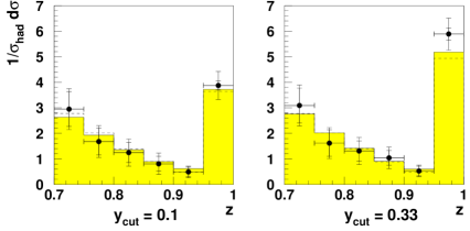
Figure 7: Comparison of the photon + 1 jet rate at leading and next-to-leading order with the ALEPH data. The non-perturbative quark-to-photon fragmentation function is fitted to the data for $y_{\rm cut}=0.06$ only. The jet rates for the other values of $y_{\rm cut}$ are then predictions from the leading order and next-to-leading order calculations.

Since the present calculation is only lowest order in the strong coupling constant, there is a large ambiguity in the choice of $\alpha_{s}$ and all values of $\alpha_{s}$ are in principle equally valid. The value $\alpha_{s}(M_{Z})=0.124$ used above was chosen such that the observed hadronic cross section can be reproduced by the ${\cal O}(\alpha_{s})$ calculation. However, jet studies at LEP have indicated that lowest order calculations of jet observables can only be matched to experimental data if a larger value of the strong coupling constant to compensate for missing higher order contributions is used. In particular, the experimental data on the isolated photon + 2, 3 jet rates [5] are well reproduced by a lowest order calculation [4] if $\alpha_{s}(M_{Z})=0.17$. We therefore provide a fit of the quark-to-photon fragmentation function for this value of $\alpha_{s}$ as well. We find

$$D_{q\to\gamma}^{np(NLO)}(z,\mu_{0})=\left(\frac{\alpha e_{q}^{2}}{2\pi}\right)\left(-P^{(0)}_{q\to\gamma}(z)\ln(1-z)^{2}+32.8(1-z)-10.35\right),$$ (10.3)

with $\mu_{0}=0.59$ GeV.

Figure  8 displays the fitted ${\cal O}(\alpha\alpha_{s})$ quark-to-photon fragmentation functions for a quark of unit charge in the $\overline{{\rm MS}}$–scheme at a factorization scale $\mu_{F}=M_{Z}$, which is the only hard scale in the process. The corresponding ${\cal O}(\alpha)$ fragmentation function obtained in [5] is shown for comparison. It is apparent that these fragmentation functions differ largely for $z\to 1$, which indicates the need for a resummation of terms proportional to $\ln(1-z)$ in this region.

Figure 8: The quark-to-photon fragmentation functions at leading and next-to-leading order as functions of $z$ for a quark of unit charge. The factorization scale $\mu_{F}$ is taken equal to $M_{Z}$ in both cases.

10.2 The integrated rate for $z>0.95$

If the photon carries a fractional momentum $z$ greater than 0.95 in the photon-jet it is considered to be isolated in the democratic clustering appoach used in the experimental ALEPH analysis. In this approach the photon is treated like any other hadron when the clustering procedure is applied to form the jets. The division between isolated and non-isolated photons suggested by ALEPH in [5] is motivated by the fact that hadronization effects smear out the isolated photon peak from $z=1$ to slightly smaller values of $z$.

This definition of isolation is in contrast with that used in previous theoretical [7, 8, 9] and experimental [6] analyses of isolated photon + $n$ jet rates, where a two-step procedure was used to define an isolated photon. In these analyses, the photon was isolated from the other hadrons using a geometrical cone before these hadrons were clustered into jets. After the clustering had taken place the photon was required to be well-separated from all of the hadronic clusters and was said to be isolated if it was accompanied only by a small amount of hadronic energy inside the cone. In these theoretical calculations [9, 8, 7], all of the quark-photon collinear and fragmentation contributions considered here were assumed to be negligible. As a result of these studies, it was found that large negative next-to-leading order corrections were needed to provide a reasonable agreement between data and theory, precisely because soft gluons were excluded from the photon cone [11].

Figure 9: The integrated photon + 1 jet rate above $z=0.95$ as function of $y_{\rm cut}$, compared with the full leading-order and next-to-leading order calculations including respectively the leading-order and next-to-leading order determined quark-to-photon fragmentation functions, $D_{q\to\gamma}(z,\mu_{F})$.

Using the fitted fragmentation function, we have evaluated the isolated photon + 1 jet rate in the democratic clustering approach up to ${\cal O}(\alpha\alpha_{s})$. The results of this calculation for the two different values of $\alpha_{s}$ are compared with the data and the leading order prediction  [4] in Fig. 9. It appears that the leading-order curve provides an adequate description of the data and that the next-to-leading order curve improves the agreement between theory and experiment over the whole range of $y_{\rm cut}$. Furthermore, it is also apparent that the next-to-leading order corrections are moderate thereby demonstrating the perturbative stability of the definition of isolation within the democratic approach.

11 Summary and Conclusions

In this paper we have presented a complete ${\cal O}(\alpha\alpha_{s})$ calculation of the photon + 1 jet rate in $e^{+}e^{-}$ annihilation. Athough this calculation is formally only next-to-leading order in perturbation theory, it contains several ingredients appropriate to next-to-next-to-leading order calculations of jet observables. For example, in addition to configurations where one final state particle is unresolved, there are also configurations where two particles are unresolved. In particular we encountered three double unresolved factors, corresponding to the triple collinear, soft/collinear and double single collinear limits of the $\gamma^{*}\to q\bar{q}g\gamma$ subprocess. To analytically isolate the singularities associated with these configurations, we employed the resolved parton philosophy of [15] and introduced a theoretical parton resolution criterion $y_{\rm min}$. These previously unknown double unresolved factors are universal and are of the type expected to arise in any calculation of jet cross sections at next-to-next-to-leading order. Matching the double unresolved parts of phase space with the single unresolved and resolved regions required some thought and was discussed at length in section 3.

All these resolved and unresolved contributions from the double bremsstrahlung process must be combined with the single unresolved contributions from one-loop and fragmentation processes. Some single and double poles in $\epsilon$ remain which have however exactly the right structure to be factorized in the next-to-leading order counterterm of the bare quark-to-photon fragmentation function.

All remaining finite contributions can then be numerically evaluated for arbitrary jet clustering algorithms. The most stringent test on the consistency of our approach is provided by Fig. 6, where it is shown that the results of the numerical program are independent of the choice of the theoretical parameter $y_{\rm min}$. This relies on the numerical cancellation of large logarithms of $y_{\rm min}$ taken up to the third power.

An important feature of this numerical program is the implementation of the hybrid subtraction method [28] which is necessary to correctly treat the overlapping of two single collinear regions in the neighberhood of double unresolved regions of the four parton phase space. This overlapping was shown to be crucial for a correct and complete coverage of all singularities in the $\gamma^{*}\to q\bar{q}\gamma g$ process in section 3.

We have presented fits of the non-perturbative part of $D_{q\to\gamma}$ for two values of $\alpha_{s}(M_{Z})$ obtained by comparing our results with the ALEPH data [5]. In determining the fragmentation function, we have required that $D_{q\to\gamma}$ is an exact solution of the ${\cal O}(\alpha\alpha_{s})$ evolution equation. This solution does not resum logarithms of the factorization scale, but does ensure that the photon + 1 jet rate is $\mu_{F}$ independent. Furthermore, at large $z$, which corresponds to the most interesting ‘isolated’ photon part of the cross section, large logarithms of $(1-z)$ are present and should be resummed.

As a first application of the fitted next-to-leading order quark-to-photon fragmentation function, we have compared the integrated ‘isolated’ photon rate for $z>0.95$ with the same ALEPH data. The theoretical next-to-leading order predictions were found to describe the data well and to provide a better agreement between theory and experiment than the leading order calculation. Furthermore, the relatively small size of the next-to-leading order corrections indicates that the isolation definition used in this democratic clustering approach is perturbatively stable.

Finally, the next-to-leading order quark-to-photon fragmentation function determined here is a universal function and appears in a variety of processes involving quarks and photons. The most prominent examples of which are the prompt photon cross section at hadron colliders and the photon pair cross section at LHC. So far the fragmentation contributions to those processes have only been evaluated using model dependent assumptions for this fragmentation function [17]. It is reasonable to expect that the fragmentation function determined directly from LEP data at high $Q^{2}$ and high $z$ should significantly improve the theoretical predictions for these processes, and, in particular, may help to determine whether a Standard Model Higgs-boson of intermediate mass can really be detected via its two photon decay at the LHC.

References

• [1] K. Koller, T.F. Walsh and P.M. Zerwas, Z. Phys. C2 (1979) 197;
E. Laermann, T.F. Walsh, I. Schmitt and P.M. Zerwas, Nucl. Phys. B207 (1982) 205.
• [2] A.D. Martin, R.G. Roberts and W.J. Stirling, Phys. Lett. B387 (1996) 419.
• [3] See for example, P. Aurenche et al. and C. Seez et al., Proceedings of the “Large Hadron Collider Workshop”, Aachen 1990, CERN report 90-10, vol. 2, p.83 and p.474.
• [4] E.W.N. Glover and A.G. Morgan, Z. Phys. C62 (1994) 311.
• [5] ALEPH collaboration: D. Buskulic et al., Z. Phys. C69 (1996) 365.
• [6] DELPHI Collaboration: P. Abreu et al., Z. Phys. C53 (1992) 555;
OPAL Collaboration: P.D. Acton et al., Z. Phys. C54 (1992) 193;
ALEPH Collaboration: D. Buskulic et al., Z. Phys. C57 (1992) 17;
L3 Collaboration: O. Adriani et al., Phys. Lett. B292 (1992) 472.
• [7] E.W.N. Glover and W.J. Stirling, Phys. Lett. B295 (1992) 128.
• [8] G. Kramer and H. Spiesberger, Proc. Workshop on “Photon Radiation from Quarks”, Annecy 1991, CERN Yellow Report 92-04, p.26.
• [9] Z. Kunszt and Z. Trócsányi, Nucl. Phys. B394 (1993) 139;
E. Berger, X. Guo and J. Qiu, Phys. Rev. D54 (1996) 5470.
• [10] E.W.N. Glover and A.G. Morgan, Phys. Lett. B334 (1994) 208.
• [11] E.W.N. Glover and A.G. Morgan, Phys. Lett. B324 (1994) 487.
• [12] A. Gehrmann–De Ridder, T. Gehrmann and E.W.N. Glover, Phys. Lett. B414 (1997) 354.
• [13] Yu.L. Dokshitzer, Contribution to the Workshop on Jets at LEP and HERA, J. Phys. G17 (1991) 1441.
• [14] K. Fabricius, I. Schmitt, G. Kramer and G. Schierholz, Z. Phys. C11 (1981) 315.
• [15] W.T. Giele and E.W.N. Glover, Phys. Rev. D46 (1992) 1980.
• [16] J. Owens, Rev. Mod. Phys. 59 (1987) 465.
• [17] M. Glück, E. Reya and A. Vogt, Phys. Rev. D48 (1993) 116;
L. Bourhis, M. Fontannaz and J.Ph. Guillet, preprint LPTHE-ORSAY 96/103 [hep-ph/9704447].
• [18] F. Bloch and A. Nordsieck, Phys. Rev. 52 (1937) 54.
• [19] T. Kinoshita, J. Math. Phys. 3 (1962) 650;
T.D. Lee and M. Nauenberg, Phys. Rev. 133 (1964) 1549.
• [20] S. Catani and M.H. Seymour, Nucl. Phys. B485 (1997) 291.
• [21] S. Frixione, Z. Kunszt and A. Signer, Nucl. Phys. B467 (1996) 399.
• [22] Z. Nagy and Z. Trócsányi, Nucl. Phys. B486 (1997) 189.
• [23] W.A. Bardeen, A.J. Buras, D.W. Duke and T. Muta, Phys. Rev. D18 (1978) 3998.
• [24] G. Altarelli and G. Parisi, Nucl. Phys. B126 (1977) 298.
• [25] G. Curci, W. Furmanski and R. Petronzio, Nucl. Phys. B175 (1980) 27;
W. Furmanski and R. Petronzio, Phys. Lett. 97B (1980) 437.
• [26] P.J. Rijken and W.L. van Neerven, Nucl. Phys. B487 (1997) 233.
• [27] A. Gehrmann-De Ridder, University of Durham Ph.D. thesis, (1997).
• [28] E.W.N. Glover and M.R. Sutton, Phys. Lett. B342 (1995) 375.
• [29] D. E. Soper and Z. Kunszt, Phys. Rev. D46 (1992) 192.
• [30] W. T. Giele, E. W. N. Glover and D. A. Kosower, Nucl. Phys. B403 (1993) 633.
• [31] E. Mirkes and D. Zeppenfeld, Phys. Lett. B380 (1996) 205.
• [32] R.K. Ellis, D.A. Ross and A.E. Terrano, Nucl. Phys. B178 (1981) 421.
• [33] Z. Bern, L. Dixon, D.C. Dunbar and D.A. Kosower, Nucl. Phys. B425 (1994) 217.
• [34] G.P. Lepage, J. Comp. Phys. 27 (1978) 192.