CERN-TH/97-142

DESY 97-090

hep-ph/9707223

NLO Production and Decay of Quarkonium
Andrea PETRELLI

INFN, Sezione di Pisa, Italy

petrelli@ibmth.difi.unipi.it

Matteo CACCIARI

Deutsches Elektronen-Synchrotron DESY, Hamburg, Germany

cacciari@desy.de

Mario GRECO

Dipartimento di Fisica E. Amaldi, Università di Roma III,

and INFN, Laboratori Nazionali di Frascati, Italy

greco@lnf.infn.it

Fabio MALTONI and Michelangelo L. MANGANO
CERN, TH Division, Geneva, Switzerland

fabio.maltoni@cern.ch, mlm@vxcern.cern.ch

We present a calculation of next-to-leading-order (NLO) QCD corrections to total hadronic production cross sections and to light-hadron-decay rates of heavy quarkonium states. Both colour-singlet and colour-octet contributions are included. We discuss in detail the use of covariant projectors in dimensional regularization, the structure of soft-gluon emission and the overall finiteness of radiative corrections. We compare our approach with the NLO version of the threshold-expansion technique recently introduced by Braaten and Chen. Most of the results presented here are new. Others represent the first independent reevaluation of calculations already known in the literature. In this case a comparison with previous findings is reported.

CERN-TH/97-142

1 Introduction

Since the discovery of the $J\!/\!\psi$ [1] and its interpretation within QCD as a charm-anticharm bound state [2], the study of quarkonium has received much attention from both a theoretical and an experimental point of view, providing a good testing ground for studies of Quantum Chromodynamics (QCD) in both its perturbative and non-perturbative regimes.

Decay rates of heavy quarkonium states into photons and light hadrons have first been calculated at leading-order (LO) and compared to experimental data (see, e.g., [3]) under the assumption of a factorization between a short-distance part describing the annihilation of the heavy-quark pair in a colour-singlet state and a non-perturbative long-distance factor, related to the value at the origin of the non-relativistic wave-function or its derivatives. Calculations of decay rates at full next-to-leading order (NLO) have also been performed in this framework since the early days of quarkonium physics [4]. This approach can be extended to the case of quarkonium production. The prescription to evaluate the short-distance coefficients is very simple: the $Q\overline{Q}$ pair has to be produced during the short-distance interaction in a colour-singlet state, with the same spin and angular momentum quantum numbers of the quarkonium state we are interested in [5]. A single non-perturbative parameter, the same appearing in the quarkonium decay and provided by the bound state Bethe-Salpeter wave-function, accounts for the hadronization of the $Q\overline{Q}$ pair into the physical quarkonium state. Applications of this approach, usually referred to as the Colour Singlet Model (CSM), led to the calculation of LO matrix elements for the production of total cross sections and $p_{T}$ distributions in hadronic collisions [6]. Phenomenological successes and failures of the CSM in describing the data available up to 1993 on charmonium production and decay are nicely reviewed in ref. [7].

In the case of $S$-waves the simple factorization hypothesis underlying the CSM was confirmed by the calculation of one loop corrections [4, 8]. The appearance of a logarithmic infrared divergence in the case of NLO $P$-wave decays into light hadrons [9, 10] violated instead factorization explicitly. Phenomenologically, this singularity could be handled by relating it to the binding energy of the bound quarks. Nevertheless, it has since then been clear that in spite of its simplicity and physical transparency, the CSM suffers from serious theoretical limitations. The principal one being the absence of a general theorem assessing its validity in higher orders of perturbation theory, as already indicated by the explicit example of $P$-states decay. The striking observation by CDF of large-$p_{T}$ $J\!/\!\psi$ and $\psi^{\prime}$ states produced at the Tevatron [11, 12] at a rate more than one order of magnitude larger than the theoretical prediction, and the serious discrepancies between fixed-target data and predictions for the relative production rates of ${}^{3}S_{1}$ ${}^{3}P_{1}$  and ${}^{3}P_{2}$  states (for recent total cross-section measurements, see [13, 14]), provided equally compelling evidence that some important piece of physics was missing from the CSM.

The road to solve these formal and phenomenological problems has been indicated by the work of Bodwin, Braaten and Lepage (BBL) [15], which provided a new framework for the study of quarkonium production and decay within QCD. In this work, perturbative factorization is retained by allowing the quarkonium production and decay to take place via intermediate $Q\overline{Q}$ states with quantum numbers different than those of the physical quarkonium state which is being produced or which is decaying. In the case of production, for example, the general expression for a cross section is given by:

$$d\sigma(H+X)=\sum_{n}d\hat{\sigma}(Q\overline{Q}[n]+X)\langle{\cal O}^{H}[n]\rangle\,.$$ (1)

Here $d\hat{\sigma}(Q\overline{Q}[n]+X)$ describes the short distance production of a $Q\overline{Q}$ pair in the colour, spin and angular momentum state $n$, and $\langle{\cal O}^{H}[n]\rangle$, the vacuum expectation value of a four-fermion operator defined within Non-Relativistic QCD (NRQCD) [16, 17], describes the hadronization of the pair into the observable quarkonium state $H$. $Q\overline{Q}$ states with quantum numbers other than $H$ arise from the expansion of the $H$ Fock-space wave function in powers of the heavy quark velocity $v$. The relative importance of the various contributions in eq. (1) can be estimated by using NRQCD velocity scaling rules [17], which allow the truncation of the series in eq. (1) at any given order of accuracy. If one only retains the lowest order in $v$, the description of $S$-wave quarkonia production or annihilation reduces to the CSM one. In the case of $P$ waves, instead, contributions from colour-octet, $S$-wave $Q\overline{Q}$ states are of the same order in $v$ as those from the leading colour-singlet $P$-wave state. Infrared singularities which appear in some of the short-distance coefficients of $P$-wave states can then be shown [15] to be absorbed into the long-distance part of colour-octet $S$-wave terms, thereby ensuring a well defined overall result. This framework for the calculation of quarkonium production and decay is often referred to as the colour-octet model (COM), perhaps with an abuse of language, as the COM pretends to be a direct outcome of QCD, rather than just a “model”. Good reviews of the underlying physical principles and applications can be found in refs. [18, 19].

The effect of colour-octet contributions can be extremely important even in the case of $S$-wave production. In fact, while their effects are predicted by the scaling rules to be suppressed by powers of $v$ with respect to the leading colour-singlet ones, their short-distance coefficients can receive contributions at lower orders of $\alpha_{s}$, thereby enhancing significantly the overall production rate [20]. The inclusion of these colour-octet processes, in conjunction with the observation that gluon fragmentation provides the dominant contribution to the short-distance coefficients at large-$p_{T}$ [21], leads to a very satisfactory description of the Tevatron data [22, 23, 24].

One of the most important consequences of factorization for quarkonium production is the prediction that the value of the non-perturbative parameters does not depend on the details of the hard process, so that parameters extracted from a given experiment can be used in different ones. For simplicity, we will refer to this concept as “universality”. Several studies of experimental data coming from different kind of reactions have been performed to assess the validity of universality. For example calculations of inclusive quarkonia production in $e^{+}e^{-}$ [25], fixed target experiments [26], $\gamma p$ collisions [27, 28] and $B$ decays [29] have been carried out within this framework. The overall agreement of theory and data is satisfactory, but there are clear indications that large uncertainties are present. The most obvious one is the discrepancy [27] between HERA data [30] and the large amount of inelastic $J\!/\!\psi$ photoproduction predicted by applying the colour-octet matrix elements extracted from the Tevatron large-$p_{T}$ data [24, 31].

It becomes therefore important to assess to which extent is universality applicable. Several potential sources of universality violation are indeed present, both at the perturbative and non-perturbative level. On one hand there are potentially large corrections to the factorization theorem itself. In the case of charmonium production, for example, the mass of the heavy quark is small enough that non-universal power-suppressed corrections can be large. Furthermore, some higher-order corrections in the velocity expansion are strongly enhanced at the edge of phase-space [32]. For example, the alternative choices of using as a mass parameter for the matrix elements and for the phase-space boundary the mass of a given quarkonium state or twice the heavy-quark mass $2m$, give rise to a large uncertainty in the production rate near threshold. These effects, which are present both in the total cross-section and in the production at large-$p_{T}$ via gluon fragmentation, violate universality. This is because the threshold behaviour depends on the nature of the hard process under consideration.

Another source of bias in the use of universality comes from purely perturbative corrections. Most of the current predictions for quarkonium production are based on the use of leading-order (LO) matrix elements. Possible perturbative $K$-factors are therefore absorbed into the non-perturbative matrix elements extracted from the comparison of data with theory. Since the size of the perturbative corrections varies from one process to the other, an artificial violation of universality is introduced. Examples of the size of these corrections are given by the large impact of $k_{T}$-kick effects and initial-state multiple-gluon emission in open-charm [33] and charmonium production [34, 35].

In this paper we focus on the evaluation of the $O(\alpha_{s}^{3})$ corrections to quarkonium total hadro-production cross sections. Of all the efforts needed to improve the quantitative estimates of quarkonium production, this is probably the less demanding one, as the formalism and the techniques to be used are a priori rather well established. Nevertheless there are some subtleties related to the regularization of the infrared (IR) and ultraviolet (UV) singularities which need to be addressed with some care. Furthermore, as pointed out in a preliminary account of part of this work [36], the impact of NLO corrections can be significant and a general study of their effects is necessary.

To carry out our calculations, we need a framework for calculating NLO inclusive production cross sections and inclusive annihilation decay rates. As well known, in perturbative calculations of the short distance coefficients beyond leading order in $\alpha_{s}$, the most convenient method for regulating both UV and IR divergences is dimensional regularization. On the other hand most calculations of production cross sections and decay rates for heavy quarkonia have been performed using the covariant projection method [5], which involves the projection of the $Q\overline{Q}$ pair onto states with definite total angular momentum $J$, and which is specific to four dimensions.

In this paper we generalize the method of covariant projection to $D=4-2\epsilon$ dimensions and perform all our calculations within this framework. Very recently a different method for calculating production cross sections and decay rates, which fully exploits the NRQCD factorization framework and bypasses the need for projections – the so called “threshold expansion method” – has been generalized to $D$ dimensions so that dimensional regularization can be used [41, 42]. We will show that, whenever common calculations exist, the results obtained using the two techniques coincide.

The knowledge of perturbative corrections to quarkonium production is rather limited. The only examples of full NLO calculations we are aware of are the following:

• total hadro-production cross-sections for ${}^{1}S_{0}$  states [37, 7];

• inclusive $p_{T}$ spectrum of $J\!/\!\psi$ in photo-production, within the CSM [38];

• corrections to the polarization of $J\!/\!\psi$ produced via gluon fragmentation [39].

In this work we present the first calculation of the $O(\alpha_{s}^{3})$ total cross-sections for hadroproduction of several $Q\overline{Q}$ states of phenomenological relevance: ${{}^{1}S_{0}}^{[8]}$, ${{}^{3}S_{1}}^{[8]}$ and ${{}^{3}P_{J}}^{[1,8]}$, where the right upper index labels the colour configuration of the $Q\overline{Q}$ pair. In addition, we repeat the calculation for ${{}^{1}S_{0}}^{[1]}$ states within our formalism, in order to establish consistency with the previous calculations of this quantity [37, 7]. We also calculate the $O(\alpha_{s}^{3})$ light-parton decay rates for ${}^{1}S_{0}$ , ${}^{3}S_{1}$  and ${}^{3}P_{J}$  colour-singlet and colour-octet states. Some of these results are new, some have been known for a long time. In the case of ${{}^{1}S_{0}}^{[1]}$ decays we find agreement with previous results [4, 8]. In the case of ${}^{3}P_{J}^{[1]}$ and ${}^{1}S_{0}^{[8]}$ decays we find a disagreement with the previous calculations, reported in [9] and in [40], respectively. While these discrepancies have a negligible numerical impact, it would be interesting to see in the future new independent calculations performed, to confirm either of the results.

This paper is structured as follows. In Section 2 we introduce our formalism, with emphasis on the extension to $D$ dimension of the covariant projection method and on its link with the NRQCD factorization approach. Section 3 gives a brief general description of the NLO calculation. In particular, we describe the technique used to identify the residues of the IR and collinear singularities and to allow their cancellation without the need for a complete $D$-dimensional calculation of the real-emission matrix elements.

Section 4 describes the behaviour of the soft limit of the NLO real corrections, and Section 5 presents the results for the various components (real and virtual corrections) of the NLO result for the decay widths. Section 6 describes how, within the NRQCD formalism, the Coulomb singularity of the virtual corrections and the aforementioned infrared singularity which appears in NLO corrections to $P$-wave decays can be disposed of. Finally, Section 7 presents the NLO results for the production processes.

Appendix A collects symbols and notations and Appendix B collects the results for the Born cross sections and decay rates in $D$ dimensions. A summary of all results is provided in Appendix C, where hadroproduction cross sections and decay widths into light hadrons are presented in their final form, after the cancellation of all singularities. In this Appendix we also comment on the discrepancies observed when comparing the results for ${}^{3}P_{0}^{[1]}$, ${}^{3}P_{2}^{[1]}$ and ${}^{1}S_{0}^{[8]}$ decays with those presented in previous calculations. Results for quarkonia photoproduction and decay into one photon plus light hadrons can be easily extracted from these calculations: explicit results will be presented in a forthcoming publication.

Appendix D presents, for comparison, a calculation of the NLO virtual corrections performed using the threshold expansion method. The results agree with those obtained using the $D$-dimensional projector technique. Appendix E presents the results for the $g\to\chi_{J}$ fragmentation function obtained within our formalism, showing again agreement with the results of the threshold expansion technique [42].

A preliminary account of some of the results contained in this paper, together with a first phenomenological study of NLO $\chi_{c,b}$ total production cross sections at fixed target and collider energies, was presented in ref. [36]. A more complete study, including the additional processes calculated in the present work, will be the subject of a separate publication.

2 Introduction to the formalism

The calculation of cross sections and decay rates for heavy quarkonia deals with two kinds of contributions: short distance ones, related to the production or annihilation of the heavy-quark pair, and long distance ones, related to non-perturbative transition between the quarks and the observable quarkonium state. Rigorous theorems exist [15] proving the factorization of these two stages in the case of inclusive quarkonium decays. Less rigorous, but widely accepted, proofs have also been given of the factorization between the perturbative and non-perturbative phases in the hadroproduction case [15]. In order to lay down the strategy of our calculation, and establish some notation, we briefly review here the essence of these factorization statements in the case of hadroproduction. Figure 1 shows a sketch of a typical diagram contributing to the inclusive production of a quarkonium state $H$. Factorization implies that we can identify an intermediate perturbative state composed of a pair of on-shell heavy quarks, whose non-perturbative evolution will lead to the formation of a physical hadron $H$ plus possibly a set $X$ of light partons. The set of light partons $Y$ consists of additional states produced during the hard collision that created the $Q\overline{Q}$ pair. Whether a light parton belongs to the set $X$ or to the set $Y$ depends on our (arbitrary) choice of factorization scale. The possibility to maintain the freedom to select this scale at all orders of perturbation theory is a consistency check of the factorization hypothesis, and leads to renormalization-group relations between the non-perturbative matrix elements which describe the long-distance physics [15]. The factorization theorem states that the effect of soft gluons exchanged between the sets $X$ and $Y$ cancel out in the production rate, and their effect can therefore be neglected. The emission of hard gluons between $X$ and $Y$, furthermore, is suppressed by powers of the ratio between the scales of the soft and hard processes.

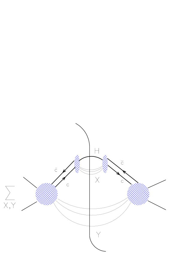
Figure 1: Diagrammatic representation of factorization in parton + parton $\to H+X$ .

At the amplitude level, and assuming the validity of the factorization theorem, the processes shown in fig. 1 can then be represented as follows:

$${\cal M}\;=\;{\cal T}_{ij}(Q\overline{Q}+Y)\;\langle H\,X|\overline{\psi_{i}}\psi_{j}|0\rangle$$ (2)

where ${\cal T}_{ij}$ is the matrix element for the production of the $Q\overline{Q}+Y$ final state with the heavy quark spinors removed, $i$ and $j$ are spinorial indices, and $\psi$ is the fermion field operator. Summing over a complete set of states containing the heavy quark pair, one then obtains:

$${\cal M}\;=\;\sum_{n}\langle H\,X|Q\overline{Q}[n]\rangle\langle Q\overline{Q}[n]|\overline{\psi_{i}}\psi_{j}|0\rangle{\cal T}_{ij}\,\equiv\;\sum_{n}\langle H\,X|Q\overline{Q}[n]\rangle\;{\mathrm{T}r}\left[\,{\cal T}\,{\mit\Pi}^{(n)}\right]\;,$$ (3)

where ${\mit\Pi^{(n)}}$ selects the quantum numbers of the quark pair relative to the state $n$. Its specific form for $S$ and $P$ wave states will be given in the following. The first term on the right-hand side is interpreted as the overlap between the perturbative $Q\overline{Q}$ state and the final hadronic state. It can be written as the transition matrix element of an operator ${\cal O}^{(n)}_{2}$, bilinear in the heavy-quark field, between the vacuum and the final state $\langle HX|$. We can therefore define the following quantity, following the notation introduced in  [15]:

$$\langle{\cal O}^{H}(n)\rangle\;=\;\sum_{X}\langle 0|{{\cal O}_{2}}^{(n)\dagger}|H\,X\rangle\langle H\,X|{{\cal O}_{2}}^{(n)}|0\rangle\;=\;\langle 0|{{\cal O}_{2}}^{(n)\dagger}{\cal P}^{H}{{\cal O}_{2}}^{(n)}|0\rangle\;,$$ (4)

where

$${\cal P}^{H}=\sum_{X}|H\,X\rangle\langle H\,X|\;.$$ (5)

We finally get the standard result [15]:

$$d\sigma(H+X)=\sum_{n}d\hat{\sigma}(Q\overline{Q}[n]+X)\langle{\cal O}^{H}(n)\rangle$$ (6)

The quantity $\langle{\cal O}^{H}(n)\rangle$ is proportional to the inclusive transition probability of the perturbative state $Q\overline{Q}[n]$ into the quarkonium state $H$. Notice that in principle we could have specified some detail of the inclusive state $X$, for example we could have specified the fraction $z$ of light-cone momentum of the pair $Q\overline{Q}[n]$ carried away by $X$, in which case we could have defined, starting from eq. (4), the equivalent of a non-perturbative fragmentation function (as opposed to an inclusive transition probability). Such a fragmentation function provides a more detailed description of the hadronization process, which can be used to parametrize potentially large higher-order $v^{2}$ corrections, such as those appearing near the boundary of phase-space. The factorization theorem allows us to extract it from some set of data, and its renormalization group properties should allow its use in different contexts. These more general non-perturbative quantities have also been introduced and discussed recently in ref. [32], where several interesting applications have been explored.

We now come to the discussion of the set of rules which define the perturbative part of eq. (6), namely the projection over the perturbative states $Q\overline{Q}[n]$. These projections have been known for some time [5] and have been used since then for the evaluation of quarkonium production and decays [6]. We will extend these rules here for use in dimensions $D=4-2\mbox{$\epsilon$}$, in view of our applications to NLO corrections, where dimensional regularization techniques are most useful to handle the appearance of infrared (IR) and ultraviolet (UV) divergences. With the exception of the normalization of spin and colour factors, discussed below, our choice of normalization is consistent with the standard non-relativistic normalizations used in [15] to define the operators entering the definition of the non-perturbative matrix elements $\langle{\cal O}^{H}(n)\rangle$.

The spin projectors for outgoing heavy quarks momenta $Q=P/2+q$ and ${\overline{Q}}=P/2-q$, are given by:

$${\mit\Pi}_{0}={1\over{\sqrt{8m^{3}}}}\left({{{P\!\!\!/}}\over 2}-{q\!\!\!/}-m\right)\gamma_{5}\left({{{P\!\!\!/}}\over 2}+{q\!\!\!/}+m\right)\,,$$ (7)

$${\mit\Pi}_{1}^{\alpha}={1\over{\sqrt{8m^{3}}}}\left({{{P\!\!\!/}}\over 2}-{q\!\!\!/}-m\right)\gamma^{\alpha}\left({{{P\!\!\!/}}\over 2}+{q\!\!\!/}+m\right)\,,$$ (8)

for spin-zero and spin-one states respectively. In these relations, $P$ is the momentum of the quarkonium state, $2q$ is the relative momentum between the $Q\overline{Q}$ pair, and $m$ is the mass of the heavy quark $Q$. The above normalization of the projection operators corresponds to a relativistic normalization of the state projected out. Higher-order powers of $q$, not required for the study of $S$ and $P$-wave states, have been neglected in eqs. (7) and (8).

The use of these operators, equal to those used in $D=4$ dimensions, requires some justification. In $D\neq 4$ dimensions, the product of two spinorial representations gives rise in fact to other representations, in addition to the spin-singlet (scalar) and spin-triplet (vector) ones. For example, the equivalent of a quarkonium state in $D=6$ can have a total spin corresponding to a scalar, a vector, and a fully-antisymmetric three-index tensor of $SO(5,1)$. The total dimension of these representations is indeed 1+5+10=16. Once we move away from $D=4$, therefore, we should in principle take into account the existence of other states in addition to the $S=0$ and $S=1$ ones found in $D=4$. For non-integer $D$, in particular, we should deal with an infinite set of states, since the Clifford algebra becomes infinite-dimensional. The projectors defined in eqs. (7,8) are still, nevertheless, the right operators needed to define the scalar and vector states. One can neglect the presence of higher-spin states in the infinite-mass limit, since spin-flip transitions, which would mix scalars and vectors to higher spins, vanish. With finite mass one can neglect the mixing among these operators provided one works at sufficiently low orders in $v$. At higher orders in $v$ spin-flip transitions occur, and in principle mixing with higher-spin states should be handled. In the calculations illustrated in this paper this never occurs, and we can safely work with just the states we are interested in, namely the $D$-dimensional scalar and vector.

The problem of dealing with the higher-spin states goes beyond the scope of this work, and will not be analyzed here in any detail. Nevertheless we want to provide some argument to suggest that even at high orders in $v$ no problems are expected. The argument proceeds as follows: higher-spin operators should vanish in 4 dimensions, and therefore their effect should be suppressed by at least one power of $\epsilon$. In order to contribute to a cross-section in 4 dimensions, they must be accompanied by some $1/\mbox{$\epsilon$}$ pole. However IR and collinear poles cannot appear: IR poles arise from the emission of soft gluons, which cannot change the spin, and collinear poles admit a factorization in terms of lower-order amplitudes times universal splitting functions. Therefore no new operators can appear in the collinear limit, and higher-spin operators should decouple. As for UV poles, in the cross-section calculations presented here they are all reabsorbed by the standard renormalization procedure. We believe it should be possible to set the above arguments on a more solid footing. We point out that a proof of the decoupling of higher-spin evanescent operators is also required when using the $D$-dimensional threshold expansion technique introduced in ref. [42], since in its current formulation the explicit assumption is made that only spin-0 and spin-1 operators are relevant.

The $D$-dimensional character of space-time is implicit in eqs. (7,8), and appears explicitly when performing the sums over polarizations, as shown later. The manipulation of expressions involving $\gamma_{5}$ is carried out by using standard techniques, as discussed in the following. The colour singlet or octet state content of a given state will be projected out by contracting the amplitudes with the following operators :

$${\cal C}_{1}={{\delta_{ij}}\over{\sqrt{{N_{c}{}}}}}\qquad{\rm for~{}the~{}singlet}$$ (9)

$${\cal C}_{8}=\sqrt{2}T_{ij}^{c}\qquad{\rm for~{}the~{}octet}$$ (10)

The projection on a state with orbital angular momentum $L$ is obtained by differentiating $L$ times the spin-colour projected amplitude with respect to the momentum $q$ of the heavy quark in the $Q\overline{Q}$ rest frame, and then setting $q$ to zero. We shall only deal with either $L=0$ or $L=1$ states, for which the amplitudes take the form:

$${\cal A}_{S=0,L=0}={\mathrm{T}r}\left.\left[{\cal C}\,{\mit\Pi}_{0}\,{\cal A}\right]\right|_{q=0}\qquad\qquad\qquad\,{\rm Spin}\;{\rm singlet}~{}S~{}{\rm states}$$ (11)

$${\cal A}_{S=1,L=0}=\epsilon_{\alpha}{\mathrm{T}r}\left.\left[{\cal C}\,{\mit\Pi}_{1}^{\alpha}\,{\cal A}\right]\right|_{q=0}\qquad\qquad\;\;\,\,\,{\rm Spin}\;{\rm triplet}~{}S~{}{\rm states}$$ (12)

$${\cal A}_{S=0,L=1}=\epsilon_{\beta}{{{\mathrm{d}}}\over{{\mathrm{d}}q_{\beta}}}{\mathrm{T}r}\left.\left[{\cal C}\,{\mit\Pi}_{0}{\cal A}\right]\right|_{q=0}\quad\qquad\;\;\,{\rm Spin}\;{\rm singlet}~{}P~{}{\rm states}$$ (13)

$${\cal A}_{S=1,L=1}={\cal E}_{\alpha\beta}{{{\mathrm{d}}}\over{{\mathrm{d}}q_{\beta}}}{\mathrm{T}r}\left.\left[{\cal C}\,{\mit\Pi}_{1}^{\alpha}{\cal A}\right]\right|_{q=0}\quad\qquad{\rm Spin}\;{\rm triplet}~{}P~{}{\rm states}$$ (14)

${\cal A}$ being the standard QCD amplitude for production (or decay) of the $Q\overline{Q}$ pair, amputated of the heavy quark spinors. The amplitudes ${\cal A}_{S,L}$ will then have to be squared, summed over the final degrees of freedom and averaged over the initial ones. The selection of the appropriate total angular momentum quantum number is done by performing the proper polarization sum. We define:

$$\Pi_{\alpha\beta}\equiv-g_{\alpha\beta}+{{P_{\alpha}P_{\beta}}\over{M^{2}}}\;,$$ (15)

where $M=2m$. The sum over polarizations for a ${}^{3}S_{1}$ state, which is still a vector even in $D=4-2\mbox{$\epsilon$}$ dimensions, is then given by:

$$\sum_{J_{z}}\mbox{$\epsilon$}_{\alpha}\mbox{$\epsilon$}_{\alpha^{\prime}}^{*}=\Pi_{\alpha\alpha^{\prime}}$$ (16)

In the case of ${}^{3}P_{J}$ states, the three multiplets corresponding to $J=0,1$ and 2 correspond to a scalar, an antisymmetric tensor and a symmetric traceless tensor, respectively. We shall denote their polarization tensors by ${\cal E}_{\alpha\beta}^{(J)}$. The sum over polarizations is then given by:

$${\cal E}_{\alpha\beta}^{(0)}{\cal E}_{\alpha^{\prime}\beta^{\prime}}^{(0)*}={1\over{D-1}}\Pi_{\alpha\beta}\Pi_{\alpha^{\prime}\beta^{\prime}}$$ (17)

$$\sum_{J_{z}}{\cal E}_{\alpha\beta}^{(1)}{\cal E}_{\alpha^{\prime}\beta^{\prime}}^{(1)*}={1\over{2}}[\Pi_{\alpha\alpha^{\prime}}\Pi_{\beta\beta^{\prime}}-\Pi_{\alpha\beta^{\prime}}\Pi_{\alpha^{\prime}\beta}]$$ (18)

$$\sum_{J_{z}}{\cal E}_{\alpha\beta}^{(2)}{\cal E}_{\alpha^{\prime}\beta^{\prime}}^{(2)*}={1\over{2}}[\Pi_{\alpha\alpha^{\prime}}\Pi_{\beta\beta^{\prime}}+\Pi_{\alpha\beta^{\prime}}\Pi_{\alpha^{\prime}\beta}]-{1\over{D-1}}\Pi_{\alpha\beta}\Pi_{\alpha^{\prime}\beta^{\prime}}$$ (19)

for the ${{}^{3}P_{0}}$, ${{}^{3}P_{1}}$ and ${{}^{3}P_{2}}$ states respectively. Total contraction of the polarization tensors gives the number of polarization degrees of freedom in $D$ dimensions. Therefore

$$N_{{}^{3}S_{1}}=\sum_{J_{z}}\mbox{$\epsilon$}_{\alpha}\mbox{$\epsilon$}_{\alpha}^{*}=\Pi_{\alpha\alpha}=D-1=3-2\mbox{$\epsilon$}$$ (20)

for the ${{}^{3}S_{1}}$ state and

$$N_{J}=\sum_{J_{z}}{\cal E}_{\alpha\beta}^{(J)}{\cal E}_{\alpha\beta}^{(J)*}$$ (21)

for the ${{}^{3}P_{J}}$ states, with

$$N_{0}=1,\;\;N_{1}={{(D-1)(D-2)}\over 2}=(3-2\mbox{$\epsilon$})(1-\mbox{$\epsilon$}),\;\;N_{2}={{(D+1)(D-2)}\over 2}=(5-2\mbox{$\epsilon$})(1-\mbox{$\epsilon$})\;.$$ (22)

The application of this set of rules produces the short-distance cross section coefficients $\hat{\sigma}$ or the short-distance decay widths $\hat{\Gamma}$ for the $ij\leftrightarrow\mbox{${}^{2S+1}L_{J}$}^{[1,8]}$ processes:

$$d\hat{\sigma}(ij\to\mbox{${}^{2S+1}L_{J}$}^{[1,8]})={1\over{2s}}\overline{\sum}|{\cal A}_{S,L}|^{2}\;d\Phi\,,$$ (23)

$$d\hat{\Gamma}(\mbox{${}^{2S+1}L_{J}$}^{[1,8]}\to ij)={1\over{4m}}\overline{\sum}|{\cal A}_{S,L}|^{2}\;d\Phi\,,$$ (24)

$s$ being the partonic centre of mass energy squared and $2m$ representing the mass of the decaying $Q\overline{Q}$ pair. To find the physical cross sections or decay rates for the observable quarkonium state $H$ these short distance coefficients must be properly related to the NRQCD production or annihilation matrix elements $\langle{\cal O}_{[1,8]}^{H}(\mbox{${}^{2S+1}L_{J}$})\rangle$ and $\langle H|{\cal O}_{[1,8]}(\mbox{${}^{2S+1}L_{J}$})|H\rangle$ respectively.

The above procedure contains some freedom in the choice of both the absolute and relative normalization of the NRQCD matrix elements. We could in fact decide to shift some overall normalization factor from the long-distance to the short-distance matrix elements. A natural choice for the absolute normalization of the non-perturbative matrix elements is obtained by requiring the short-distance coefficients to coincide with those which appear when the expectation value of the NRQCD operators is taken between free $Q\overline{Q}$ states. The relative normalization between colour-singlet and colour-octet operators is obtained by imposing the decomposition:

$${{\cal{O}}}_{\rm tot}={{\cal{O}}}_{1}+{{\cal{O}}}_{8}\;.$$ (25)

The identification of the colour-singlet and color-octet components is obtained by using the Fierz rearrangement:

$$\delta_{i^{\prime}i}\delta_{j^{\prime}j}={1\over{N_{c}{}}}\delta_{ji}\delta_{i^{\prime}j^{\prime}}+2T^{a}_{ji}T^{a}_{i^{\prime}j^{\prime}}$$ (26)

The identification of the spin-0 and spin-1 components is obtained by using the Fierz rearrangement:

$$\delta_{i^{\prime}i}\delta_{j^{\prime}j}={1\over 2}\left[\delta_{ji}\delta_{i^{\prime}j^{\prime}}+\sigma^{a}_{ji}\sigma^{a}_{i^{\prime}j^{\prime}}\right]\;,$$ (27)

with the normalization of the Pauli matrices fixed to the canonical one:

$$\left\{\sigma^{a}\,,\,\sigma^{b}\right\}\;=\;2\delta^{ab}\;.$$ (28)

Combining the two results, we obtain the following decomposition:

$$\psi^{\dagger}\psi\;\chi^{\dagger}\chi = {1\over 2{N_{c}{}}}\left(\psi^{\dagger}\chi\;\chi^{\dagger}\psi\;+\;\psi^{\dagger}\sigma^{i}\chi\;\chi^{\dagger}\sigma^{i}\psi\right)$$ (29)

$$+ \psi^{\dagger}T^{a}\chi\;\chi^{\dagger}T^{a}\psi\;+\;\psi^{\dagger}T^{a}\sigma^{i}\chi\;\chi^{\dagger}T^{a}\sigma^{i}\psi\;.$$

We find it natural to use this decomposition to identify the normalization of the NRQCD operators, which are presented in full detail for $S$ and $P$-wave states in Appendix A. The resulting normalization for the colour-singlet part differs from the usual one found in the literature. Compared to the conventions of BBL [15], our normalizations are given by:

$${{\cal{O}}}_{1}={{{\cal{O}}}_{1}^{\rm BBL}\over 2{N_{c}{}}},$$ (30)

$${{\cal{O}}}_{8}={{\cal{O}}}_{8}^{\rm BBL}.$$ (31)

We stress that, in addition to being more natural, (e.g. in the case of $S$ waves the non-perturbative matrix elements for colour singlet states coincide exactly with the value of the total wave functions evaluated at the origin), our definition is probably more adequate when trying to estimate the order of magnitude of non-perturbative matrix elements using velocity-scaling rules. For example, it is known that the ratio between the matrix elements of the colour-octet and colour-singlet ${}^{3}S_{1}$ operators should scale like $v^{4}$. The extraction of $\langle{\cal{O}}^{\psi,{\rm BBL}}_{8}({{}^{3}S_{1}})\rangle$ from the Tevatron data [23, 24, 31] leads to values in the range $0.65\div 1.4\times 10^{-2}$ GeV^-3. The value of $\langle{\cal{O}}^{\psi,{\rm BBL}}_{1}({{}^{3}S_{1}})\rangle$ is given by 1.3 GeV^-3. The ratio between the two, of the order of $0.5\div 1\times 10^{-2}$, is quite smaller than the estimated value of $v^{4}\sim 0.06$. Using our normalization of the NRQCD operators, the ratio becomes $3\div 6\times 10^{-2}$, which is consistent with the velocity scaling rule. This behaviour is confirmed by similar results obtained in the case of $\psi^{\prime}$ and $P$-wave states.

Having done this, the cross sections and the decay rates read:

$$\sigma(ij\to\mbox{${}^{2S+1}L_{J}$}^{[1,8]}\to H)=\hat{\sigma}(ij\to\mbox{${}^{2S+1}L_{J}$}^{[1,8]}){{\langle{\cal{O}}_{[1,8]}^{H}(\mbox{${}^{2S+1}L_{J}$})\rangle}\over{N_{col}N_{pol}}},$$ (32)

$$\Gamma(H\to\mbox{${}^{2S+1}L_{J}$}^{[1,8]}\to ij)=\hat{\Gamma}(\mbox{${}^{2S+1}L_{J}$}^{[1,8]}\to ij)\langle H|{\cal{O}}_{[1,8]}(\mbox{${}^{2S+1}L_{J}$})|H\rangle.$$ (33)

$N_{col}$ and $N_{pol}$ refer to the number of colours and polarization states of the $Q\overline{Q}[\mbox{${}^{2S+1}L_{J}$}]$ pair produced. They are given by 1 for singlet states or $N_{c}^{2}-1$ for octet states, and by the $D$-dimensional $N_{J}$’s defined above. Dividing by these colour and polarization degrees of freedom in the cross sections is necessary as we had summed over them in the evaluation of the short distance coefficient $\hat{\sigma}$. Analogously, these degrees of freedom are summed over in the decay matrix element, but averaged as part of the definition of the short distance width $\hat{\Gamma}$, when mediating over the $Q\overline{Q}$ initial state.

The matrix elements appearing in the equations above are of course meant to be the bare $D$-dimensional ones whenever $D$-dimensional cross sections or decay rates are to be calculated. Making use of their correct mass dimension, $3-2\mbox{$\epsilon$}$ and $5-2\mbox{$\epsilon$}$ for $S$ and $P$ wave states respectively (see Section 6), gives the right dimensionality to $D$-dimensional cross sections and widths, i.e. $2-D=-2+2\mbox{$\epsilon$}$ and 1, respectively.

2.1 Digression on the use of $\gamma_{5}$ in dimensional regularization

Once the right counting of degrees of freedom is taken into account via the polarization sums eqs. (17,18,19) , further potential inconsistencies which could, a priori, spoil the possibility of using projectors on $D$-dimensional amplitudes, are related to the the definition of the matrix $\gamma_{5}$ in arbitrary dimensions. Several prescriptions have been introduced and shown to be consistent in specific problems. The most common ones are the naive dimensional regularization (NDR) [43] and the t’Hooft-Veltman dimensional regularization (HVDR)  [44].

Within the first prescription, $\gamma_{5}^{N}$ is defined by the property that it anti-commutes with all $\gamma^{\mu}$ in $D$ dimensions

$$\{\gamma_{5}^{N},\gamma^{\mu}\}=0\,,\qquad\mu=0,1,\cdots,D-1,$$ (34)

and it satisfies

$$(\gamma_{5}^{N})^{2}=1\,.$$ (35)

while, in contrast to (34), in the t’Hooft-Veltman prescription it holds

$$\gamma_{5}^{HV}\equiv i\gamma^{0}\gamma^{1}\gamma^{2}\gamma^{3}\,,$$ (36)

and

$$\{\gamma_{5}^{HV},\gamma^{\mu}\} = 0\,,\;\;\;\mu=0,1,2,3\,,$$ (37)

$$\left[\gamma_{5}^{HV},\gamma^{\mu}\right] = 0\,,\;\;\;\mu=4,\cdots,D-1\,.$$ (38)

Since it is defined explicitly by construction in eq. (36), $\gamma_{5}^{HV}$ is unique and well-defined, while to this respect, $\gamma_{5}^{N}$, is an ambiguous object. For example, while the HVDR scheme allows to recover the standard Adler-Bell-Jackiw anomaly, the NDR does not without additional ad hoc prescriptions.

We do not expect any ambiguity to arise in our case, since in QCD parity is conserved and since no $\gamma_{5}$ insertions are present inside the loop amplitudes we will be evaluating. Extra care should instead be applied when dealing with, for example, corrections to the decay $b\to{\cal Q}_{c\bar{c}}\,s$. To verify the independence from the scheme, we did the calculation of virtual diagrams contributing to NLO decay widths and cross sections of ${}^{1}S_{0}^{[1,8]}$ states in both in the HVDR and NDR schemes. The results were found to coincide exactly, diagram by diagram.

Finally we would like to compare our technique with the ones available in the literature. Braaten and Chen [41, 42] determine the short-distance coefficients via the matching technique, generalizing to $D-1$ spatial dimensions their threshold expansion method. This technique is briefly presented in Appendix D and has been used in this paper as a check for the virtual contributions in the NLO calculations. Within this approach a quantity that is closely related to the cross section for the production of a $Q\overline{Q}$ pair with total momentum $P$ is calculated using perturbation theory in full QCD and expanded in powers of the relative 3-momentum ${\bf q}$ of the $Q\overline{Q}$ pair and in a few non relativistic matrix elements. To exploit this procedure one is forced to choose a representation for $\gamma$-matrices. Braaten and Chen write

$$\gamma^{0}\;=\;\left(\begin{array}[]{cc}1&0\\ 0&-1\end{array}\right)\;,\qquad\gamma^{i}\;=\;\left(\begin{array}[]{cc}0&\sigma^{i}\\ -\sigma^{i}&0\end{array}\right)\;,\quad i=1,\dots D-1\;.$$ (39)

Once this choice has been made, one easily realizes that no room is left for selecting a $\gamma_{5}$ different from

$$\gamma_{5}^{BC}\;=\;\left(\begin{array}[]{cc}0&1\\ 1&0\end{array}\right)\;,$$ (40)

which, as a simple calculation shows, satisfies eq. (34). This observation shows that in the $D$-dimensional threshold expansion method an implicit choice for dealing with $\gamma_{5}$ is made and it exactly corresponds to $\gamma_{5}^{BC}=\gamma_{5}^{N}$.

3 General description of the calculation of higher-order corrections

In this section we briefly describe the strategy of the calculation of higher-order corrections to decay widths and to total production cross sections. The reader who is not interested in the details of the calculation, can just read this section to get an idea of the general framework, and can skip the following sections where all the required calculations are carried out.

A consistent calculation of higher-order corrections entails the evaluation of the real and virtual emission diagrams, carried out in $D$ dimensions. The UV divergences present in the virtual diagrams are removed by the standard renormalization. The IR divergences appearing after the integration over the phase space of the emitted parton are cancelled by similar divergences present in the virtual corrections, or by higher order corrections to the long-distance matrix elements [15]. Collinear divergences, finally, are either cancelled by similar divergences in the virtual corrections or, in the case of production, by factorization into the NLO parton densities. The evaluation of the real emission matrix elements in $D$ dimensions is usually particularly complex, and is presumably the main reason that has prevented the so far the calculation of NLO corrections to the production of $P$-wave states. In this paper we follow an approach already employed in [45], whereby the structure of soft and collinear singularities in $D$ dimensions is extracted by using universal factorization properties of the amplitudes. Thanks to these factorization properties, that will be discussed in detail in the following section, the residues of all IR and collinear poles in $D$ dimensions can be obtained without an explicit calculation of the full $D$-dimensional real matrix elements. They only require, in general, knowledge of the $D$-dimensional Born-level amplitudes, a much simpler task. The isolation of these residues allows to carry out the complete cancellations of the relative poles in $D$ dimensions, leaving residual finite expressions which can then be evaluated exactly directly in $D=4$ dimensions. In this way one can avoid the calculation of the full $D$-dimensional real-emission matrix elements. Furthermore, the four-dimensional real matrix elements that will be required have been known in the literature for quite some time [6, 24].

4 Soft emission behaviour

We discuss in this section the factorization properties of the real-emission amplitudes in the soft-emission limit. The factorization formulae presented here will be used in the following sections to isolate the IR poles and cancel them against the singularities of the virtual processes.

Figure 2: Diagrams for the $q\overline{q}$ and $gg$ Born amplitudes.

4.1 Soft factorization in $3g$ amplitudes

We start by considering the case of decays into gluons. At the Born level, the relevant diagrams are shown in fig. 2. The decay amplitude (before projection on a specific quarkonium state) can be written as follows:

$$A_{\rm Born}\;=\;(ab)_{ij}\;(D_{1}+D_{3})\;+\;(ba)_{ij}\;(D_{2}-D_{3})\;,$$ (41)

where we introduced the short-hand notation:

$$(a\dots b)_{ij}\;=\;\left(T_{a}\dots T_{b}\right)_{ij}\;,$$ (42)

where the $T^{a}$ matrices are normalized according to ${\mathrm{T}r}(T^{a}T^{b})=\delta^{ab}/2$ (more details on our conventions for the colour algebra can be found in Appendix A). The terms $D_{1}$, $D_{2}$ and $D_{3}$ correspond to the three diagrams appearing in fig. 2 with the colour coefficients removed. Using this notation, the amplitude for emission of a soft gluon with momentum $k$ and colour label $c$ can be written as follows [46]:

$$A_{\rm soft} = g(cab)_{ij}\left[{Q\epsilon_{c}\over Qk}-{a\epsilon_{c}\over ak}\right](D_{1}+D_{3})+g(acb)_{ij}\left[{a\epsilon_{c}\over ak}-{b\epsilon_{c}\over bk}\right](D_{1}+D_{3})$$ (43)

$$+ g(abc)_{ij}\left[{b\epsilon_{c}\over bk}-{\overline{Q}\epsilon_{c}\over\overline{Q}k}\right](D_{1}+D_{3})+g(cba)_{ij}\left[{Q\epsilon_{c}\over Qk}-{b\epsilon_{c}\over bk}\right](D_{2}-D_{3})$$

$$+ g(bca)_{ij}\left[{b\epsilon_{c}\over bk}-{a\epsilon_{c}\over ak}\right](D_{2}-D_{3})+g(bac)_{ij}\left[{a\epsilon_{c}\over ak}-{\overline{Q}\epsilon_{c}\over\overline{Q}k}\right](D_{2}-D_{3})\;,$$

where $Q$ and $\overline{Q}$ are the momenta of the heavy quarks, and $a$, $b$ indicate the momenta and colour labels of the final state gluons.

In the case of $S$-wave decay we can set $Q=\overline{Q}=P/2$. All terms proportional to $Q\epsilon_{c}~{}$or to $\overline{Q}\epsilon_{c}~{}$vanish in the transverse gauge defined by the gauge vector $(k_{0},-\vec{k})$. The soft-emission amplitude becomes:

$$A_{\rm soft} = g\left[([a,c]b)_{ij}\,{a\epsilon_{c}\over ak}-(a[c,b])_{ij}\,{b\epsilon_{c}\over bk}\right](D_{1}+D_{3})$$ (44)

$$+ g\left[([b,c]a)_{ij}\,{b\epsilon_{c}\over bk}-(b[c,a])_{ij}\,{a\epsilon_{c}\over ak}\right](D_{2}-D_{3})\;.$$

In the case of ${}^{3}P$-wave decays we also need the derivative of the decay amplitude with respect to the relative momentum of the quark and antiquark. In the soft-gluon limit, we obtain:

$$\left({dA_{\rm soft}\over dq_{\alpha}}\right)_{q=0} = g\left[([a,c]b)_{ij}\,{a\epsilon_{c}\over ak}-(a[c,b])_{ij}\,{b\epsilon_{c}\over bk}\right]{d(D_{1}+D_{3})\over dq_{\alpha}}$$ (45)

$$+ g\left[([b,c]a)_{ij}\,{b\epsilon_{c}\over bk}-(b[c,a])_{ij}\,{a\epsilon_{c}\over ak}\right]{d(D_{2}-D_{3})\over dq_{\alpha}}$$

$$+ 2g\,{\epsilon_{c}^{\alpha}\over Pk}\left\{\left[(abc)_{ij}+(cab)_{ij}\right](D_{1}+D_{3})+\left[(bac)_{ij}+(cba)_{ij}\right](D_{2}-D_{3})\right\}$$

It is easy to prove with an explicit calculation that the two terms proportional to $\epsilon_{c}^{\alpha}$ give vanishing contributions, in the soft-gluon limit, when projected on all ${}^{3}P_{J}$ states. Therefore the structure of the soft limit of the derivative of the amplitude is similar to that of the amplitude itself.

We now proceed to prove explicitly the factorization of the soft-gluon emission probability. We will indicate with $\overline{D}_{i}$ ($i=1,2,3$) the projection of the diagrams $D_{i}$ on a given quarkonium state, and with $\overline{A}_{\rm Born}$ and $\overline{A}_{\rm soft}$ the projected amplitudes for the Born and soft-emission processes, respectively.

The colour coefficients for the decay of a colour-singlet state can be obtained by using the projector $\delta_{ij}\delta_{kl}/{N_{c}{}}$. The colour-singlet amplitudes therefore become:

$$\overline{A^{[1]}_{\rm Born}} = {1\over 2{N_{c}{}}}\delta_{ab}\delta_{ij}(\overline{D}_{1}+\overline{D}_{2})\;,$$ (46)

$$\overline{A^{[1]}_{\rm soft}} = {igf^{acb}\over 2{N_{c}{}}}\delta_{ij}\left[{a\epsilon_{c}\over ak}-{b\epsilon_{c}\over bk}\right](\overline{D}_{1}+\overline{D}_{2})\;,$$ (47)

and simple colour algebra gives the final result for the soft-emission:

$$\sum_{\rm col,pol}\;|\overline{A^{[1]}_{\rm soft}}|^{2}\;=\;{2ab\over(ak)(bk)}{C_{A}{}}g^{2}\sum_{\rm col,pol}\;|\overline{A^{[1]}_{\rm Born}}|^{2}$$ (48)

The colour-octet case can be obtained from the following relation:

$$\sum_{\rm col,pol}\;|\overline{A^{[8]}}|^{2}\;=\;\sum_{\rm col,pol}\;|\overline{A}|^{2}\;-\;\sum_{\rm col,pol}\;|\overline{A^{[1]}}|^{2}$$ (49)

The first term on the right-hand side can be easily obtained with standard colour algebra, and the final result is:

$$\sum_{\rm col,pol}\;|\overline{A^{[8]}_{\rm soft}}|^{2}\;=\;{C_{A}{}}g^{2}\left[{2ab\over(ak)(bk)}-{2ab\over(Pk)^{2}}\right]\sum_{\rm col,pol}\;|\overline{A^{[8]}_{\rm Born}}|^{2}$$ (50)

4.2 Soft factorization in light-quark processes

An approach similar to that used in the previous subsection can be applied to the case of soft-gluon emission in processes where the $Q\overline{Q}$ pair ${\cal{Q}}$ decays into light-quark pairs (${\cal{Q}}\to\mbox{$q\overline{q}$}$). The Born-level amplitude (which is non-vanishing only in the colour-octet case) is given by:

$$A_{\rm Born}\;=\;{1\over 2}\left[\delta_{ik}\delta_{jl}-{1\over{N_{c}{}}}\delta_{ij}\delta_{kl}\right]D_{0}\;,$$ (51)

where $(i,j)$ and $(k,l)$ are the color indices of heavy and light quark pairs, respectively, and where $D_{0}$ is shown in fig. 2, with the colour factors removed and before projection onto the quarkonium quantum numbers. The amplitude for emission of a soft gluon with momentum $k$ and colour label $c$ can be written as follows:

$$A_{\rm soft}\;=\;gD_{0}\!\!\!\!\!\!\! \left\{{T^{c}_{ik}\over 2}\delta_{jl}\left[{Q\epsilon_{c}\over Qk}-{q\epsilon_{c}\over qk}\right]\;+\;{T^{c}_{jl}\over 2}\delta_{ik}\left[{\overline{q}\epsilon_{c}\over\overline{q}k}-{\overline{Q}\epsilon_{c}\over\overline{Q}k}\right]\right.$$ (52)

$$-\left.{T^{c}_{ij}\over 2{N_{c}{}}}\delta_{kl}\left[{Q\epsilon_{c}\over Qk}-{\overline{Q}\epsilon_{c}\over\overline{Q}k}\right]\;+\;{T^{c}_{kl}\over 2{N_{c}{}}}\delta_{ij}\left[{q\epsilon_{c}\over qk}-{\overline{q}\epsilon_{c}\over\overline{q}k}\right]\right\}\;.$$

The colour-singlet and colour-octet projections are then given by:

$$A^{[1]}_{\rm soft} = {gD_{0}\over 2{N_{c}{}}}T^{c}_{ij}\delta_{lk}\left[{Q\epsilon_{c}\over Qk}-{\overline{Q}\epsilon_{c}\over\overline{Q}k}\right]$$ (53)

$$A^{[8]}_{\rm soft} = A_{\rm soft}-A^{[1]}_{\rm soft}\;.$$ (54)

We study first the case of $S$-wave decays. As before, we can set to zero all terms proportional to $Q\epsilon_{c}~{}$and $\overline{Q}\epsilon_{c}~{}$by choosing a transverse gauge. The colour-singlet amplitude obviously vanishes, and the colour-octet one reduces itself to:

$$A_{\rm soft}\;=\;{gD_{0}\over 2}\left\{\left[T^{c}_{ik}\delta_{jl}-{1\over{N_{c}{}}}T^{c}_{kl}\delta_{ij}\right]{q\epsilon_{c}\over qk}+\left[T^{c}_{lj}\delta_{ik}-{1\over{N_{c}{}}}T^{c}_{kl}\delta_{ij}\right]{\overline{q}\epsilon_{c}\over\overline{q}k}\right\}\;.$$ (55)

An explicit calculation gives the following factorization formula, which is non-vanishing only in the ${}^{3}S_{1}$ case since the ${}^{1}S_{0}$ Born amplitude vanishes:

$$\sum_{\rm col,pol}\;|\overline{A^{[8]}_{\rm soft}}|^{2}\;=\;g^{2}\;\sum_{\rm col,pol}|\overline{A^{[8]}_{\rm Born}}|^{2}\left[{2q\bar{q}\over(qk)(\bar{q}k)}{C_{F}{}}-{2M^{2}\over(Pk)^{2}}{{C_{A}{}}\over 2}\right]\,,$$ (56)

where $M=2m$.

In the case of $P$ waves we need to consider as well the derivative with respect to the relative momentum of the heavy quarks:

$$\left({dA_{\rm soft}\over dq_{\alpha}}\right)_{q=0}\;=\;gD_{0}\left({\epsilon_{c}^{\alpha}\over Pk}-{k^{\alpha}\over(Pk)^{2}}(P\epsilon_{c})\right)\left[T^{c}_{ik}\delta_{jl}+T^{c}_{lj}\delta_{ik}-{2\over{N_{c}{}}}T^{c}_{ij}\delta_{kl}\right]\;.$$ (57)

The terms proportional to $dD_{0}/dq_{\alpha}$ vanish because $D_{0}$ corresponds to an $S$-wave process. Denoting by $\cal{C}$ the overall colour coefficient in the previous equation, choosing a transverse gauge where $\epsilon_{c}\cdot P=0$ and using the projection operators for ${}^{3}P_{J}$-waves given in section 2, we obtain the following result for the quarkonium-decay amplitude:

$$\overline{A_{\rm soft}}(^{3}P_{J})\;=\;g{1\over Pk}{\cal C}\;\overline{A_{\rm Born}}(^{3}S_{1}(\epsilon_{\rm eff}))\;.$$ (58)

The amplitude was written in terms of the amplitude for the production of a ${}^{3}S_{1}$ colour-octet state, with an effective polarization $\epsilon_{\rm eff}$ given in terms of the polarizations of the soft gluon and of the ${}^{3}P_{J}$ state as follows:

$$\epsilon^{J}_{{\rm eff},\beta}\;=\;\epsilon_{c}^{\alpha}{\cal E}_{\alpha\beta}^{J}(P)\;.$$ (59)

The correlations between the polarization of the gluon and of the ${\cal Q}$ state induce a dependence of the soft-emission amplitude on the relative direction of the gluon and of the light quarks. Nevertheless, if we average over the soft gluon $D-1$ spatial directions we get:

$$\int{d\Omega^{D-1}_{k}\over\Omega^{D-1}}\sum_{\rm pol}\epsilon_{c}^{\alpha}\epsilon_{c}^{\beta*}={D-2\over D-1}\Pi_{\alpha\beta}(P)\;,$$ (60)

and one can easily compute the sum over effective polarizations

$$\int{d\Omega^{D-1}_{k}\over\Omega^{D-1}}\sum_{\epsilon_{c}}\epsilon^{J}_{{\rm eff},\alpha}\epsilon^{J*}_{{\rm eff},\beta}=-N_{J}{D-2\over D-1}\Pi_{\alpha\beta}(P)\;.$$ (61)

Here $N_{J}$ is the number of degrees of freedom of the ${}^{3}P_{J}$ state in $D$ dimensions. With the above expressions at hand, it is straightforward to square the amplitude in eq. (58) and obtain

$$\int d\Omega^{D-1}_{k}\overline{\sum}|A_{\rm soft}(^{3}P_{J})|^{2}=\Omega^{D-1}{(D-2)^{2}\over(D-1)^{2}}\overline{\sum_{\rm colours}}|{\cal C}|^{2}{4g^{2}\over(Pk)^{2}}\,N_{J}\,\overline{\sum}|A_{\rm Born}(^{3}S_{1}^{[8]})|^{2}\,\,,$$ (62)

The above formula embodies the well known singular behaviour of the $P$-wave decay into light quarks [10], to be absorbed into the colour-octet ${}^{3}S_{1}$ NRQCD matrix element, as shown in ref. [15] and discussed in Section 6. This formula also shows that this phenomenon is present not only for colour-singlet $P$ wave states, but for colour octet ones as well. The colour factors (averaged over initial states) are given by:

$$\overline{\sum_{\rm colours}}|{{\cal C}^{[1]}}|^{2} = {C_{F}{}}\;,$$ (63)

$$\overline{\sum_{\rm colours}}|{{\cal C}^{[8]}}|^{2} = {B_{F}{}}\;,$$ (64)

for the colour-singlet and colour-octet cases, respectively. ${C_{F}{}}$ and ${B_{F}{}}$ are defined in Appendix A.

5 Decay Processes at NLO

The previous study of the soft behaviour of the real-emission amplitudes will now be used to calculate the full set of NLO corrections to decay and production of quarkonium states. The general factorization formulae that we proved in the previous section will be useful to efficiently extract the singular behaviour of the real-emission amplitudes, using the general formalism of refs. [45]. In conjunction with the universal behaviour of amplitudes in the collinear regions, the knowledge of the residues of the soft singularities will enable us to extract all poles of infrared and collinear origin, cancel them against the poles in the virtual amplitudes and in the parton densities, and be left with finite terms which only depend on the real-emission matrix elements in 4 dimensions. This technique saves us from the complex evaluation of the full matrix elements for real emission in $D$ dimensions. In this section we confine ourselves to the case of decay rates. We will discuss the production cross-sections in Section 7.

5.1 Real emission corrections in $D$ dimensions

5.1.1 Kinematics and factorization of soft and collinear singularities

Let us consider the three-body decay processes ${\cal{Q}}^{[1,8]}\to k_{1}+k_{2}+k_{3}$, where ${\cal{Q}}^{[1,8]}\equiv Q\overline{Q}[\mbox{${}^{2S+1}L_{J}$}^{[1,8]}]$. They are described in terms of the invariants

$$x_{i}={2Pk_{i}\over M^{2}}\,,\quad\quad\sum x_{i}=2\,,$$ (65)

where $P$ is the momentum of the decaying $Q\overline{Q}$ pair of mass $M=2m$. The three-body phase space in $D=4-2\epsilon$ dimensions is given by:

$$d\Phi_{(3)} = {M^{2}\over 2(4\pi)^{3}}\;\left({4\pi\over M^{2}}\right)^{2\epsilon}\;{1\over\Gamma(2-2\epsilon)}\;\prod_{i=1}^{3}\,(1-x_{i})^{-\epsilon}\,dx_{i}\delta(2-\sum x_{i})$$ (66)

$$= \Phi_{(2)}{N\over K}\prod_{i=1}^{3}\,(1-x_{i})^{-\epsilon}\,dx_{i}\delta(2-\sum x_{i})\;,$$

where $\Phi_{(2)}$ is the total two-body phase space in $D$ dimensions:

$$\Phi_{(2)}\;=\;{1\over 8\pi}\left({4\pi\over M^{2}}\right)^{\epsilon}\;{\Gamma(1-\epsilon)\over\Gamma(2-2\epsilon)}\;,$$ (67)

and $N$ and $K$ are defined as

$$N = {M^{2}\over(4\pi)^{2}}\;\left({4\pi\over M^{2}}\right)^{\epsilon}\;\Gamma(1+\epsilon)\;,$$ (68)

$$K = \Gamma(1+\epsilon)\Gamma(1-\epsilon)\sim 1+\epsilon^{2}{\pi^{2}\over 6}\;.$$ (69)

For future reference, it is useful to define as well the following function:

$$f_{\epsilon}(M^{2})\;=\;\left({4\pi\mu^{2}\over M^{2}}\right)^{\epsilon}\;\Gamma(1+\epsilon)\;,$$ (70)

where $\mu$ is the renormalization scale.

Collinear and soft singularities in the matrix element squared

$${\cal{M}}(x_{1},x_{2},x_{3})\;=\;\overline{\sum}|A(x_{1},x_{2},x_{3})|^{2}$$ (71)

appear as single poles in either of the terms $1-x_{i}$. As a consequence, the function

$$f(x_{1},x_{2},x_{3})\;=\;\prod_{i=1}^{3}\,(1-x_{i}){\cal{M}}(x_{1},x_{2},x_{3})$$ (72)

will be finite throughout the phase space. In terms of the function $f$, the differential decay width can be written as:

$$d\Gamma\;=\;{\Phi_{(2)}\over 2M}\,{N\over K}\prod_{i=1}^{3}\,(1-x_{i})^{-1-\epsilon}\,dx_{i}\,\delta(2-\sum x_{i})\,f(x_{1},x_{2},x_{3})\;.$$ (73)

It is useful to introduce the variables $(x,y,z)$, defined by:

$$x_{1} = 1-xy$$ (74)

$$x_{2} = 1-x(1-y)$$ (75)

$$x_{3} = z$$ (76)

With these variables

$$\prod_{i=1}^{3}\,(1-x_{i})\;=\;x^{2}\,(1-x)\,y\,(1-y)\;,$$ (77)

$$\prod_{i=1}^{3}\,dx_{i}\,\delta(2-\sum x_{i})\;=\;xdx\,dy\;,$$ (78)

with $z=x$. The total decay width can then be written as:

$$\Gamma\;=\;{\Phi_{(2)}\over 2M}\,{N\over K}\,{1\over{\cal{S}}}\int_{0}^{1}d\,x\int_{0}^{1}d\,y\;x^{-1-2\epsilon}\,(1-x)^{-1-\epsilon}\,\left[y(1-y)\right]^{-1-\epsilon}f(x,y)\,$$ (79)

where $\cal{S}$ is a symmetry factor, equal to $3!$ in the case of 3-gluon decays, and equal to 1 in the case of $g\mbox{$q\overline{q}$}$ decays. The function

$$f(x,y)\equiv f(x_{1}=1-xy,x_{2}=1-x+xy,x_{3}=x)$$ (80)

is finite for all values of $x$ and $y$ within the integration domain. Therefore all singularities of the total decay rate can be easily extracted by isolating the $\epsilon\to 0$ poles from the factors in eq.(79) explicitly depending on $x$ and $y$, as discussed in the next subsection.

5.1.2 Colour-singlet three-gluon decays

For the sake of definiteness, we present now the detailed calculations relative to the decay of a colour singlet state into three gluons. The colour octet can be worked out in a similar manner, and will be given with fewer details in the following.

To exploit the total symmetry of the three gluons in the final state we restrict the integration to the domain $x_{3}<x_{1},x_{2}$. In terms of the variables $x$ and $y$, this corresponds to

$$0<x<{2\over 3}\quad,\quad 2-{1\over x}<y<{1\over x}-1\;.$$ (81)

This choice corresponds to integrating over one third of the entire phase space, multiplying the result by the multiplicity factor 3. To proceed, we make use of the following expansions valid for small $\epsilon$:

$$x^{-1-2\epsilon}\;=\;-{4^{\epsilon}\over 2\epsilon}\delta(x)+\left({1\over x}\right)_{1/2}\,-\,2\epsilon\left({\log\,x\over x}\right)_{1/2}\,+\,{\cal{O}}(\epsilon^{2})\,.$$ (82)

where we introduced the “1/2” distributions defined as follows:

$$\int_{0}^{1/2}\,dx\,\left[d(x)\right]_{1/2}t(x)\;=\;\int_{0}^{1/2}\,dx\;d(x)\;\left[t(x)-t(0)\right]\;.$$ (83)

We then obtain:

$$x^{-1-2\epsilon}\,(1-x)^{-\epsilon}=-{4^{\epsilon}\over 2\epsilon}\delta(x)+\left({1\over x}\right)_{1/2}-\epsilon\left\{{\log(1-x)\over x}+2\left[{\log\,x\over x}\right]_{1/2}\right\}\,+\,{\cal O}(\epsilon^{2})$$ (84)

The total decay width can then be written as the sum of three terms:

$$\Gamma\;=\;\Gamma_{x=0}+\Gamma_{0<x<1/2}+\Gamma_{1/2<x<2/3}\;,$$ (85)

where

$$\Gamma_{x=0} = -{4^{\epsilon}\over 2\epsilon}{\Phi_{(2)}\over 2M}\,{N\over K}\,{3\over{\cal{S}}}\int_{0}^{1}d\,y\;\,\left[y(1-y)\right]^{-1-\epsilon}f(0,y)$$ (86)

$$\Gamma_{0<x<1/2} = {\Phi_{(2)}\over 2M}\,{N\over K}\,{3\over{\cal{S}}}\int_{0}^{1/2}d\,x\int_{0}^{1}d\,y\;\,\left[y(1-y)\right]^{-1-\epsilon}{f(x,y)\over(1-x)}$$ (87)

$$\times\,\left[\left({1\over x}\right)_{1/2}-\epsilon\left\{{\log(1-x)\over x}+2\left[{\log\,x\over x}\right]_{1/2}\right\}\right]\,$$

$$\Gamma_{1/2<x<2/3} = {\Phi_{(2)}\over 2M}\,{N\over K}\,{3\over{\cal{S}}}\int_{1/2}^{2/3}d\,x\int_{2-1/x}^{1/x-1}d\,y\;{1\over x(1-x)y(1-y)}f(x,y)\,.$$ (88)

Notice that the last term is finite, since no pole is present within the integration domain. It can therefore be computed directly in 4-dimensions.

We shall now proceed to the evaluation of each of these terms, starting from the first one. The $x\to 0$ limit is the soft limit for $k_{3}$. In this limit, eq.(48) gives:

$${\cal{M}}(x,y)\;\stackrel{{\scriptstyle x\to 0}}{{\longrightarrow}}\;{16\pi{C_{A}{}}\mbox{$\alpha_{s}^{(b)}$}\over M^{2}}\,{1\over x^{2}y(1-y)}\,{\cal{M}}_{\rm Born}\;,$$ (89)

where $\mbox{$\alpha_{s}^{(b)}$}=\mbox{$\alpha_{s}$}\mu^{2\epsilon}$ is the dimensional coupling constant in $D$ dimensions and ${\cal{M}}_{\rm Born}$ is the Born amplitude squared and averaged in $D$ dimensions for the ${\cal{Q}}\to gg$ processes. As a result,

$$\Gamma_{x=0} \equiv -{4^{\epsilon}\over 2\epsilon}{1\over 2M}{\Phi_{(2)}\over 2!}{N\over K}\int\,dy\,\left[y(1-y)\right]^{-1-\epsilon}f(x=0,y)$$ (90)

$$= \,{1\over 2M}{\Phi_{(2)}\over 2!}{N\over K}\,{16\pi{C_{A}{}}\mbox{$\alpha_{s}^{(b)}$}\over M^{2}}\,\mbox{${\cal{M}}_{\rm Born}$}\,\left({1\over\epsilon^{2}}\;+{2\over\epsilon}\log\,2+\,2\log^{2}\,2-\,{\pi^{2}\over 3}\right)\;.$$ (91)

In the cases in which $\mbox{${\cal{M}}_{\rm Born}$}=0$, such as for example ${\cal{Q}}={{}^{3}P_{1}}$, $\mbox{${\cal{M}}_{\rm Born}$}=0$ and the left-hand side of the above equation, together with $\Gamma_{x=0}$, vanish.

In order to evaluate $\Gamma_{0<x<1/2}$, we use the following relation:

$$\left[y(1-y)\right]^{-1-\epsilon}\;=\;-{1\over\epsilon}\left[\delta(y)+\delta(1-y)\right]+\left[\left({1\over y}\right)_{+}+\left({1\over 1-y}\right)_{+}\right]\,+\,{\cal{O}}(\epsilon)$$ (92)

With obvious notation, we can therefore decompose $\Gamma_{0<x<1/2}$ as follows:

$$\Gamma_{0<x<1/2}\;=\;\Gamma_{y=0}+\Gamma_{y=1}+\Gamma_{\rm{finite}}\;.$$ (93)

The limits $y\to 0$ and $y\to 1$ correspond to the collinear limits $k_{2}\parallel k_{3}$ and $k_{1}\parallel k_{3}$, respectively. In these limits we can apply the universal factorization of collinear singularities

$$f(x,y=0)\;=\;f(x,y=1)\;=\;{8\pi\mbox{$\alpha_{s}^{(b)}$}\over M^{2}}\;P_{gg}(x)\;\mbox{${\cal{M}}_{\rm Born}$}\,x(1-x)\;,$$ (94)

where $P_{gg}(x)$ is the $D$-dimensional Altarelli-Parisi splitting kernel:

$$P_{gg}(x)\;=\;2{C_{A}{}}\left[{x\over 1-x}+{1-x\over x}+x(1-x)\right]\;,$$ (95)

and obtain the following result:

$$\Gamma_{y=0}\;=\;\Gamma_{y=1} = {16\pi\mbox{$\alpha_{s}^{(b)}$}{C_{A}{}}\over M^{2}}{1\over 2M}{\Phi_{(2)}\over 2!}{N\over K}\mbox{${\cal{M}}_{\rm Born}$}$$ (96)

$$\times\left[{11\over 12\epsilon}-{1\over\epsilon}\log\,2+{45\over 16}-{\pi^{2}\over 4}+{11\over 12}\log\,2-\log^{2}\,2\,\right]\;.$$

We can now collect all the results obtained so far in the following expression

$$\Gamma({\cal{Q}}\to 3g)\;=\;\Gamma^{[1]}_{\rm{univ}}+\Gamma_{\rm{finite}}\;,$$ (97)

where

$$\Gamma^{[1]}_{\rm{univ}} \equiv \left[\Gamma_{x=0}+\Gamma_{y=0}+\Gamma_{y=1}\right]$$ (98)

$$= {{C_{A}{}}\mbox{$\alpha_{s}$}\over\pi}\,\mbox{$\Gamma_{\rm Born}$}\,f_{\epsilon}(M^{2})\,\left({1\over\epsilon^{2}}+{11\over 6\epsilon}+{45\over 8}-{5\over 6}\pi^{2}+{11\over 6}\log\,2\right)$$

is a universal term, whose dependence on the quarkonium type is only implicit in the factor $\Gamma_{\rm Born}$, and where

$$\Gamma_{\rm{finite}}\;=\;{1\over 2M}{\Phi_{(2)}\over 2!}{N\over K}\int_{0}^{{1\over 2}}\,dx\,\int_{0}^{1}\,dy\,f(x,y)\left[\left({1\over y}\right)_{+}+\left({1\over 1-y}\right)_{+}\right]\left({1\over x}\right)_{{1\over 2}}+\;\Gamma_{1/2<x<2/3}$$ (99)

is a finite expression, explicitly dependent on the quarkonium state through the specific form of the function $f(x,y)$. In particular, this is the only term which survives in cases where $\mbox{${\cal{M}}_{\rm Born}$}=0$, consistently with the form taken by eq.(79) in the limit $\epsilon\to 0$. Since $\Gamma_{\rm{finite}}$ is free of soft and collinear singularities, it can be evaluated directly in four dimensions. In particular, this implies that the matrix elements for the real process ${\cal{Q}}\to ggg$ can be calculated in $D=4$ dimensions, with a significant reduction in the complexity of the calculation. The evaluation of the $\Gamma_{\rm{finite}}$ contributions is a tedious but straightforward calculation, which makes use of the 4-dimensional matrix elements given in ref. [6] for the colour-singlet states. The explicit evaluation leads to the following result (valid for $\mbox{$\Gamma_{\rm Born}$}\neq 0$):

$$\Gamma({\cal{Q}}^{[1]}\to ggg)\;=\;{{C_{A}{}}\mbox{$\alpha_{s}$}\over\pi}\Gamma_{\rm Born}({\cal{Q}}^{[1]}\to gg)f_{\epsilon}(M^{2})\left({1\over\epsilon^{2}}+{11\over 6\epsilon}+A^{[1]}_{{\cal{Q}}}\right)\;,$$ (100)

with

$$A^{[1]}_{{{}^{1}S_{0}}}\;=\;{181\over 18}-{23\over 24}\pi^{2}\;,$$ (101)

$$A^{[1]}_{{{}^{3}P_{0}}}\;=\;{400\over 81}-{61\over 144}\pi^{2}\;,$$ (102)

$$A^{[1]}_{{{}^{3}P_{2}}}\;=\;{2113\over 216}-{401\over 384}\pi^{2}\;.$$ (103)

The processes ${{}^{3}S_{1}}\to ggg$ and ${{}^{3}P_{1}}\to ggg$ are completely finite. In absence of real or virtual contributions from two-gluon final states, they provide the LO contribution to the gluonic decay rates:

$$\Gamma^{H}({{}^{3}S_{1}}^{[1]}\to ggg) = 4\,\mbox{$\alpha_{s}^{3}$}\,C_{2}(F)\left(-1+{\pi^{2}\over 9}\right){{\langle H|{\cal{O}}_{1}({{}^{3}S_{1}})|H\rangle}\over{m^{2}}}$$ (104)

$$\Gamma^{H}({{}^{3}P_{1}}^{[1]}\to ggg) = \mbox{$\alpha_{s}^{3}$}\,{C_{A}{}}\,{C_{F}{}}\left({587\over 27}-{317\over 144}\pi^{2}\right){{\langle H|{\cal{O}}_{1}({{}^{3}P_{1}})|H\rangle}\over{m^{4}}}.$$ (105)

These results agree with previous evaluations (see e.g. Schuler [7]).

We would like to point out an interesting fact related to the size of the non-universal finite corrections appearing in eqs. (101) through (105): although the size of the contributions from the rational number and from the term proportional to $\pi^{2}$ are large in each case, there is always a cancellation between them which reduces their sum to about 1/10 of their individual value. The same accurate cancellations take place in the processes that will be considered in the following subsections. In all cases the finite coefficient $A^{[1,8]}_{{\cal{Q}}}$ is a number of order 1.

5.1.3 Colour-octet three-gluon decays

The case of colour-octet decays can be analysed in a similar way, the only difference being in the soft limit of the amplitude squared, given by eq.(50):

$${\cal{M}}(x,y)\;\stackrel{{\scriptstyle x\to 0}}{{\longrightarrow}}\;{16\pi{C_{A}{}}\mbox{$\alpha_{s}^{(b)}$}\over M^{2}}\,{1-y(1-y)\over x^{2}y(1-y)}\,{\cal{M}}_{\rm Born}\;,$$ (106)

where ${\cal{M}}_{\rm Born}$ is the Born amplitude squared and averaged in $D$ dimensions for the ${\cal{Q}}^{[8]}\to gg$ processes. Following the same steps as above, we get:

$$\Gamma({\cal{Q}}^{[8]}\to 3g)\;=\;\Gamma^{[8]}_{\rm{univ}}+\Gamma_{\rm{finite}}\;,$$ (107)

where

$$\Gamma^{[8]}_{\rm{univ}}\;=\;{{C_{A}{}}\mbox{$\alpha_{s}$}\over\pi}\,\mbox{$\Gamma_{\rm Born}$}\,f_{\epsilon}(M^{2})\left({1\over\epsilon^{2}}+{7\over 3\epsilon}+{53\over 8}-{5\over 6}\pi^{2}+{17\over 6}\log\,2\right)\,,$$ (108)

is the universal term for colour octet decays. Once the finite part is calculated, making use of the 4-dimensional amplitudes derived in ref. [24], we obtain the following results:

$$\Gamma({\cal{Q}}^{[8]}\to ggg)\;=\;{{C_{A}{}}\mbox{$\alpha_{s}$}\over\pi}\mbox{$\Gamma_{\rm Born}$}({\cal{Q}}^{[8]}\to gg)f_{\epsilon}(M^{2})\left({1\over\epsilon^{2}}+{7\over 3\epsilon}+A^{[8]}_{{\cal{Q}}}\right)\;,$$ (109)

with

$$A^{[8]}_{{{}^{1}S_{0}}}\;=\;{104\over 9}-\pi^{2}\;,$$ (110)

$$A^{[8]}_{{{}^{3}P_{0}}}\;=\;{875\over 162}-{10\over 27}\pi^{2}\;,$$ (111)

$$A^{[8]}_{{{}^{3}P_{2}}}\;=\;{4679\over 432}-{73\over 72}\pi^{2}\;.$$ (112)

The processes ${{}^{3}P_{1}}^{[8]}\to ggg$ and ${{}^{3}S_{1}}^{[8]}\to ggg$ are completely finite because of the vanishing of two-gluon amplitudes. They read:

$$\Gamma^{H}({{}^{3}P_{1}}^{[8]}\to ggg)=\mbox{$\alpha_{s}^{3}$}\;{C_{A}{}}\,{B_{F}{}}\left({1369\over 54}-{23\over 9}\pi^{2}\right){{\langle H|{\cal{O}}_{8}({{}^{3}P_{1}})|H\rangle}\over{m^{4}}}\,,$$ (113)

$$\Gamma^{H}({{}^{3}S_{1}}^{[8]}\to ggg)=5\;\mbox{$\alpha_{s}^{3}$}\left(-{73\over 4}+{67\over 36}\pi^{2}\right){{\langle H|{\cal{O}}_{8}({{}^{3}S_{1}})|H\rangle}\over{m^{2}}}\,.$$ (114)

5.1.4 Colour singlet $\mbox{$q\overline{q}$}g$ decays

The ${{}^{1}S_{0}}^{[1]}\to\mbox{$q\overline{q}$}g$ decay rate can be calculated along the same lines as above, starting from eq. (79). No soft-gluon pole is present for $x\to 0$, and the collinear singularities are extracted by using the Altarelli-Parisi factorization. The result is given by:

$$\Gamma^{H}({{}^{1}S_{0}}^{[1]}\to\mbox{$q\overline{q}$}g)={n_{f}{}}\Gamma^{H}_{\rm Born}({{}^{1}S_{0}}^{[1]}\to gg){\mbox{$\alpha_{s}$}\over\pi}{f_{\epsilon}(M^{2})\over K}{T_{F}{}}\left[-{2\over 3\epsilon}-{16\over 9}\right]\,.$$ (115)

The process ${{}^{3}S_{1}}^{[1]}\to\mbox{$q\overline{q}$}g$ is equal to zero. The results for $P$-wave colour-singlet states are given by:

$$\Gamma^{H}(\mbox{${}^{3}P_{J}^{[1]}$}\to q\overline{q}g)={n_{f}{}}\Gamma^{H}_{\rm Born}(\mbox{${}^{3}P_{J}^{[1]}$}\to gg){\mbox{$\alpha_{s}$}\over\pi}{f_{\epsilon}(M^{2})\over K}{T_{F}{}}\left(-{2\over 3\epsilon}\right)$$

$$-{4\over 9}{n_{f}{}}{C_{F}{}}\mbox{$\alpha_{s}^{3}$}{\mu^{2\mbox{$\epsilon$}}\langle H|{\cal{O}}_{1}(^{3}P_{J})|H\rangle\over m^{4}}\left[{1\over\epsilon}{f_{\epsilon}(M^{2})\over K}\left({4\pi\mu^{2}\over M^{2}}\right)^{\epsilon}{\Gamma(1-\epsilon)\over\Gamma(2-2\epsilon)}+a_{J}\right]\,$$ (116)

where

$$a_{0}={28\over 3}\;\;,\;\;a_{1}={7\over 3}\;\;,\;\;a_{2}={53\over 15}$$ (117)

and $f_{\epsilon}$ is defined in Appendix  A.

In the above equations the $1/\mbox{$\epsilon$}$ poles proportional to ${T_{F}{}}$ are due to the gluon splitting into collinear quarks. They will be cancelled by the virtual corrections to the two-gluon decay process. The singular $J$-independent pieces, proportional to ${C_{F}{}}$, come from the soft-gluon pole isolated in eq. (62), and will be cancelled by the addition of the ${{}^{3}S_{1}}^{[8]}\to\mbox{$q\overline{q}$}$ contribution to the decay width (see Section 6).

5.1.5 Colour octet $\mbox{$q\overline{q}$}g$ decays

The process ${{}^{1}S_{0}}^{[8]}\to\mbox{$q\overline{q}$}g$ is completely analogous to the colour singlet one:

$$\Gamma^{H}({{}^{1}S_{0}}^{[8]}\to\mbox{$q\overline{q}$}g)={n_{f}{}}\Gamma^{H}_{\rm Born}({{}^{1}S_{0}}^{[8]}\to gg){\mbox{$\alpha_{s}$}\over\pi}{f_{\epsilon}(M^{2})\over K}{T_{F}{}}\left[-{2\over 3\epsilon}-{16\over 9}\right]\,.$$ (118)

The process ${{}^{3}S_{1}}^{[8]}\to\mbox{$q\overline{q}$}g$ shows collinear and IR singularities that are expected to cancel against the virtual ones:

$$\Gamma^{H}({{}^{3}S_{1}}^{[8]}\to q\overline{q}g) = \Gamma^{H}_{\rm Born}({{}^{3}S_{1}}^{[8]}\to q\overline{q}){\mbox{$\alpha_{s}$}\over\pi}f_{\epsilon}(M^{2})\left\{{C_{F}{}}\left({1\over\mbox{$\epsilon$}^{2}}+{3\over 2\mbox{$\epsilon$}}\right)+{C_{A}{}}{1\over 2\mbox{$\epsilon$}}\right.$$ (119)

$$+\left.{C_{F}{}}\left({19\over 4}-{2\over 3}\pi^{2}\right)+{11\over 6}{C_{A}{}}\right\}\,.$$

The colour-octet $P$-wave decays exhibit the same singularity structure as the colour-singlet case, and are given by:

$$\Gamma^{H}(\mbox{${}^{3}P_{J}^{[8]}$}\to q\overline{q}g)={n_{f}{}}\Gamma^{H}_{\rm Born}(\mbox{${}^{3}P_{J}^{[8]}$}\to gg){\mbox{$\alpha_{s}$}\over\pi}{f_{\epsilon}(M^{2})\over K}{T_{F}{}}\left(-{2\over 3\epsilon}\right)$$

$$-{4\over 9}{n_{f}{}}{B_{F}{}}\mbox{$\alpha_{s}^{3}$}{\mu^{2\mbox{$\epsilon$}}\langle H|{\cal{O}}_{8}(^{3}P_{J})|H\rangle\over m^{4}}\left[{1\over\epsilon}{f_{\epsilon}(M^{2})\over K}\left({4\pi\mu^{2}\over M^{2}}\right)^{\epsilon}{\Gamma(1-\epsilon)\over\Gamma(2-2\epsilon)}+a_{J}\right]$$ (120)

and the quantities $a_{J}$ are defined in (117). ${B_{F}{}}$ is defined in Appendix A.

5.2 Virtual corrections

We present in this section the results of the calculation of the 1-loop diagrams necessary for the evaluation of the virtual corrections to the production and decay matrix elements. The final results for the decay rates, obtained by combining the results of this section with those on real emission presented in the previous sections, are collected in Appendix C.

The explicit calculation of the virtual contribution $\Gamma_{V}$ was done using dimensional regularization, both for the UV and the IR divergences. We have introduced the parameter $v$ defined in the Appendix A in order to regularize the Coulomb singularity. The quantity $v$ represents the velocity of the heavy quarks in the quarkonium rest frame, and is kept small but finite. The Coulomb singularities appear as poles in the relative velocity, i.e. as $1/2v$. The relevant Feynman diagrams are shown in figures  3 and  4, and the results are given diagram by diagram in tables 1, 2, 3 and 4. In these tables we report the contribution of each diagram $k$, indicating separately the colour factors $f_{k}$ relative to the colour singlet and colour octet cases.

The expressions ${\cal D}_{k}$ appearing in the tables are defined by the following equation:

$$\Gamma_{V}\;=\;\mbox{$\Gamma_{\rm Born}$}{\mbox{$\alpha_{s}$}\over\pi}f_{\epsilon}(M^{2})\sum_{k}\mbox{${\cal D}_{k}$}\mbox{$f_{k}$}\;,$$ (121)

where the sum extends over the set of diagrams.

The virtual corrections are both infrared and ultraviolet divergent. While the infrared poles are cancelled when adding the real corrections, the ultraviolet ones are instead disposed of via coupling constant and heavy quark mass renormalization. The latter has already been explicitly performed in the on-shell scheme, which amounts to replacing the bare mass by

$$m^{\rm bare}=m\left[1-{3\mbox{$\alpha_{s}$}\over 4\pi}{C_{F}{}}\left({1\over\mbox{$\epsilon_{\!\!\mbox{ \tiny{UV} }}$}}-\gamma_{E}+\log 4\pi+{4\over 3}\right)\right]\,.$$ (122)

The coupling constant renormalization has instead been left undone, to give in principle anyone the possibility to perform it in a scheme of his own choice. We will do it in the ${\overline{\rm MS}}$ scheme through the replacement of the bare coupling constant by

$$\mbox{$\alpha_{s}^{(b)}$}=\mu^{2\mbox{$\epsilon$}}\mbox{$\alpha_{s}$}\left[1-{\mbox{$\alpha_{s}$}\over 2\pi}b_{0}\left({1\over\mbox{$\epsilon_{\!\!\mbox{ \tiny{UV} }}$}}-\gamma_{E}+\log 4\pi\right)\right]\,.$$ (123)

We point out that we carried out the evaluation of the virtual corrections using two independent techniques. In addition to using the $D$-dimensional projection operators constructed in sec. 2, we also used the threshold-expansion technique introduced in ref. [41, 42], and reviewed here in Appendix  D. The results obtained in the two cases coincide exactly, diagram by diagram, providing an important consistency check of our calculation showing the equivalence of our $D$-dimensional projections to the threshold expansion method.

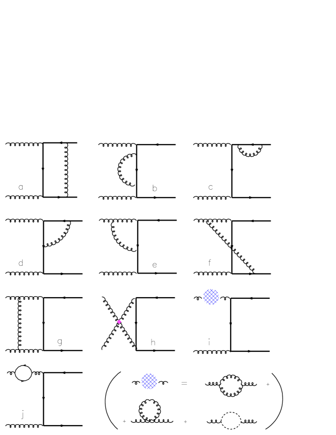
Figure 3: Feynman diagrams contributing to the one-loop corrections to the processes $Q\overline{Q}[^{3}P_{0}^{[1,8]}]\to gg$, $Q\overline{Q}[^{3}P_{2}^{[1,8]}]\to gg$ and $Q\overline{Q}[^{1}S_{0}^{[1,8]}]\to gg$.

5.2.1 Colour-singlet $gg$ virtual decays

The singularity structure of the virtual corrections is dictated by the renormalization properties of the theory, by the universal form of the Coulomb limit, and by requirement that soft and collinear singularities cancel against the real corrections evaluated above. The form of the virtual corrections to the decay rate is therefore the following:

$$\Gamma_{V}^{H}({\cal{Q}}^{[1]}\to gg) = \mbox{$\Gamma_{\rm Born}^{H}$}({\cal{Q}}^{[1]}\to gg){\mbox{$\alpha_{s}$}\over\pi}f_{\epsilon}(M^{2})$$ (124)

$$\times\left\{{b_{0}\over\epsilon_{\rm UV}}+{C_{F}{}}{\pi^{2}\over 2v}-{C_{A}{}}\left({1\over\epsilon^{2}}+{11\over 6\epsilon}\right)+{2\over 3\epsilon}{n_{f}{}}{T_{F}{}}+B^{[1]}_{{\cal{Q}}}\right\}\;,$$

where we explicitly labelled the $\epsilon$’s to indicate their origin, and where all of the state dependence is included in the finite factor $B_{{\cal{Q}}}$. The heavy quark-antiquark relative velocity $2v$, $b_{0}$ and $f_{\epsilon}(M^{2})$ are defined in Appendix A. ${n_{f}{}}$ is the number of flavours lighter than the heavy, bound one, as a consequence of the heavy quark never appearing in the virtual loops.

Diag.	${\cal D}_{k}$	$f_{k}^{[1]}$	$f_{k}^{[8]}$
a	${\pi^{2}\over 2v}+{1\over\mbox{$\epsilon$}}-2+2\log 2$	${C_{F}{}}$	$C_{F}-{1\over 2}C_{A}$
b	$-{1\over 2\mbox{$\epsilon_{\!\!\mbox{ \tiny{UV} }}$}}-1+3\log 2$	$C_{F}$	$C_{F}$
c	$-{1\over 2\mbox{$\epsilon_{\!\!\mbox{ \tiny{UV} }}$}}-{1\over\mbox{$\epsilon$}}-2-3\log 2$	$C_{F}$	$C_{F}$
d	${1\over\mbox{$\epsilon_{\!\!\mbox{ \tiny{UV} }}$}}-2\log 2+{\pi^{2}\over 4}$	$C_{F}-{1\over 2}C_{A}$	$C_{F}-{1\over 2}C_{A}$
e	$-{3\over\mbox{$\epsilon_{\!\!\mbox{ \tiny{UV} }}$}}+{1\over\mbox{$\epsilon$}^{2}}+{1\over\mbox{$\epsilon$}}-4+2\log 2-{\pi^{2}\over 6}$	$-{1\over 2}$$C_{A}$	$-{1\over 2}$$C_{A}$
f	${1\over\mbox{$\epsilon$}^{2}}+{1\over\mbox{$\epsilon$}}+2-4\log 2-{5\over 12}\pi^{2}$	${1\over 2}{C_{A}{}}$	$0$
g	$-{1\over\mbox{$\epsilon$}^{2}}-{1\over\mbox{$\epsilon$}}-2+2\log 2+{2\over 3}\pi^{2}$	$C_{A}$	${1\over 2}{C_{A}{}}$
h	$0$	$C_{A}$	$C_{A}$
i	${5\over 6\mbox{$\epsilon_{\!\!\mbox{ \tiny{UV} }}$}}-{5\over 6\mbox{$\epsilon$}}$	$C_{A}$	${C_{A}{}}$
j	$\left(-{2\over 3\mbox{$\epsilon_{\!\!\mbox{ \tiny{UV} }}$}}+{2\over 3\mbox{$\epsilon$}}\right){n_{f}{}}$	$T_{F}$	$T_{F}$

Table 1: First column: diagram labels according to the conventions of fig. 3. Second column: diagram-by-diagram contribution to the virtual corrections to the matrix element squared for the processes $Q\overline{Q}[^{1}S_{0}^{[1,8]}]\to gg$ and with colour factors set to 1. Third column: colour factors relative to the $gg$ colour singlet decay. Fourth column: colour factors relative to the $gg$ colour octet decay.

Diag.	${\cal D}_{k}$	$f_{k}^{[1]}$	$f_{k}^{[8]}$
a	${\pi^{2}\over 2v}+{1\over\mbox{$\epsilon$}}-{4\over 9}+{32\over 9}\log 2+{\pi^{2}\over 12}$	${C_{F}{}}$	$C_{F}-{1\over 2}C_{A}$
b	$-{1\over 2\mbox{$\epsilon_{\!\!\mbox{ \tiny{UV} }}$}}-{13\over 9}+{5\over 9}\log 2$	$C_{F}$	$C_{F}$
c	$-{1\over 2\mbox{$\epsilon_{\!\!\mbox{ \tiny{UV} }}$}}-{1\over\mbox{$\epsilon$}}-2-3\log 2$	$C_{F}$	$C_{F}$
d	${1\over\mbox{$\epsilon_{\!\!\mbox{ \tiny{UV} }}$}}+{14\over 9}-{10\over 9}\log 2+{\pi^{2}\over 6}$	$C_{F}-{1\over 2}C_{A}$	$C_{F}-{1\over 2}C_{A}$
e	$-{3\over\mbox{$\epsilon_{\!\!\mbox{ \tiny{UV} }}$}}+{2\over 3\mbox{$\epsilon$}^{2}}+{20\over 9\mbox{$\epsilon$}}-{11\over 3}+{2\over 3}\log 2-{\pi^{2}\over 9}$	$-{1\over 2}$$C_{A}$	$-{1\over 2}$$C_{A}$
f	${4\over 3\mbox{$\epsilon$}^{2}}-{2\over 9\mbox{$\epsilon$}}+1-{20\over 3}\log 2-{5\over 9}\pi^{2}$	${1\over 2}{C_{A}{}}$	$0$
g	$-{4\over 3\mbox{$\epsilon$}^{2}}+{2\over 9\mbox{$\epsilon$}}-{14\over 27}+{14\over 27}\log 2+{13\over 18}\pi^{2}$	$C_{A}$	${1\over 2}{C_{A}{}}$
h	$-{19\over 27}+{70\over 27}\log 2$	$C_{A}$	$C_{A}$
i	${5\over 6\mbox{$\epsilon_{\!\!\mbox{ \tiny{UV} }}$}}-{5\over 6\mbox{$\epsilon$}}$	$C_{A}$	${C_{A}{}}$
j	$\left(-{2\over 3\mbox{$\epsilon_{\!\!\mbox{ \tiny{UV} }}$}}+{2\over 3\mbox{$\epsilon$}}\right){n_{f}{}}$	$T_{F}$	$T_{F}$

Table 2: Same as table 1, for ${}^{3}P_{0}^{[1,8]}$ states.

Diag.	${\cal D}_{k}$	$f_{k}^{[1]}$	$f_{k}^{[8]}$
a	${\pi^{2}\over 2v}+{1\over\mbox{$\epsilon$}}-{5\over 3}+{7\over 3}\log 2+{\pi^{2}\over 8}$	${C_{F}{}}$	$C_{F}-{1\over 2}C_{A}$
b	$-{1\over 2\mbox{$\epsilon_{\!\!\mbox{ \tiny{UV} }}$}}-{1\over 6}+{11\over 6}\log 2$	$C_{F}$	$C_{F}$
c	$-{1\over 2\mbox{$\epsilon_{\!\!\mbox{ \tiny{UV} }}$}}-{1\over\mbox{$\epsilon$}}-2-3\log 2$	$C_{F}$	$C_{F}$
d	${1\over\mbox{$\epsilon_{\!\!\mbox{ \tiny{UV} }}$}}-{1\over 6}-{7\over 6}\log 2-{\pi^{2}\over 8}$	$C_{F}-{1\over 2}C_{A}$	$C_{F}-{1\over 2}C_{A}$
e	$-{3\over\mbox{$\epsilon_{\!\!\mbox{ \tiny{UV} }}$}}+{3\over 8\mbox{$\epsilon$}^{2}}+{17\over 16\mbox{$\epsilon$}}-{59\over 96}-{\pi^{2}\over 16}$	$-{1\over 2}$$C_{A}$	$-{1\over 2}$$C_{A}$
f	${13\over 8\mbox{$\epsilon$}^{2}}+{15\over 16\mbox{$\epsilon$}}+{107\over 96}-{11\over 2}\log 2-{67\over 48}\pi^{2}$	${1\over 2}{C_{A}{}}$	$0$
g	$-{13\over 8\mbox{$\epsilon$}^{2}}-{15\over 16\mbox{$\epsilon$}}-{17\over 288}+{89\over 18}\log 2+{37\over 48}\pi^{2}$	$C_{A}$	${1\over 2}{C_{A}{}}$
h	$-{5\over 9}-{10\over 9}\log 2$	$C_{A}$	$C_{A}$
i	${5\over 6\mbox{$\epsilon_{\!\!\mbox{ \tiny{UV} }}$}}-{5\over 6\mbox{$\epsilon$}}$	$C_{A}$	${C_{A}{}}$
j	$\left(-{2\over 3\mbox{$\epsilon_{\!\!\mbox{ \tiny{UV} }}$}}+{2\over 3\mbox{$\epsilon$}}\right){n_{f}{}}$	$T_{F}$	$T_{F}$

Table 3: Same as table 1, for ${}^{3}P_{2}^{[1,8]}$ states.

Summing the contribution of all diagrams, we obtain the following results for the colour singlet coefficients $B_{{\cal{Q}}}^{[1]}$ :

$$B^{[1]}_{{{}^{1}S_{0}}}\;=\;\;{C_{F}{}}\left(-5+{\pi^{2}\over 4}\right)+{C_{A}{}}\left(1+{5\over 12}\pi^{2}\right)\,,$$ (125)

$$B^{[1]}_{{{}^{3}P_{0}}}\;=\;{C_{F}{}}\left(-{7\over 3}+{\pi^{2}\over 4}\right)+{C_{A}{}}\left({1\over 3}+{5\over 12}\pi^{2}\right)\;,$$ (126)

$$B^{[1]}_{{{}^{3}P_{2}}}\;=\;-4{C_{F}{}}+{C_{A}{}}\left({1\over 3}+{5\over 3}\log 2+{\pi^{2}\over 6}\right)\;.$$ (127)

We recall that the virtual corrections to processes which are absent at the Born level vanish.

5.2.2 Colour-octet virtual $gg$ decays

Summing the contributions in tables 1, 2 and 3, we get the following result for the colour-octet $gg$ decays:

$$\Gamma_{V}^{H}({\cal{Q}}^{[8]}\to gg) = \mbox{$\Gamma_{\rm Born}^{H}$}({\cal{Q}}^{[8]}\to gg){\mbox{$\alpha_{s}$}\over\pi}f_{\epsilon}(M^{2})$$ (128)

$$\times\left\{{b_{0}\over\epsilon_{\rm UV}}+(\mbox{$C_{F}-{1\over 2}C_{A}$}){\pi^{2}\over 2v}-{C_{A}{}}\left({1\over\epsilon^{2}}+{7\over 3\epsilon}\right)+{2\over 3\epsilon}{n_{f}{}}{T_{F}{}}+B^{[8]}_{{\cal{Q}}}\right\}\;,$$

where the state-dependent finite parts are given by:

$$B^{[8]}_{{{}^{1}S_{0}}}\;=\;\;{C_{F}{}}\left(-5+{\pi^{2}\over 4}\right)+{C_{A}{}}\left(2+{7\over 24}\pi^{2}\right)\,,$$ (129)

$$B^{[8]}_{{{}^{3}P_{0}}}\;=\;{C_{F}{}}\left(-{7\over 3}+{\pi^{2}\over 4}\right)+{C_{A}{}}\left({17\over 54}+{35\over 27}\log 2+{7\over 24}\pi^{2}\right)\;,$$ (130)

$$B^{[8]}_{{{}^{3}P_{2}}}\;=\;-4{C_{F}{}}+{C_{A}{}}\left({23\over 36}+{7\over 9}\log 2+{5\over 12}{\pi^{2}}\right)\;.$$ (131)

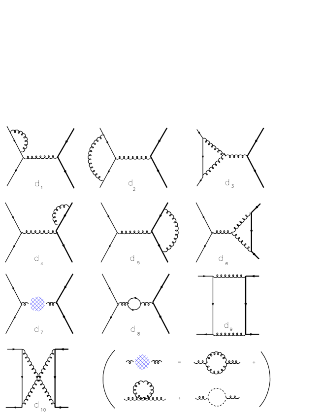
Figure 4: Feynman diagrams contributing to the one-loop corrections to the process $\mbox{$q\overline{q}$}\to Q\overline{Q}[^{3}S_{1}^{[8]}]$.

Diag.	${\cal D}_{k}$	$f_{k}$
$d_{1}$	$-{1\over 2\mbox{$\epsilon_{\!\!\mbox{ \tiny{UV} }}$}}+{1\over 2\mbox{$\epsilon$}}$	${C_{F}{}}$
$d_{2}$	${1\over 2\mbox{$\epsilon_{\!\!\mbox{ \tiny{UV} }}$}}-{1\over{\mbox{$\epsilon$}}^{2}}-{2\over\mbox{$\epsilon$}}-4+{2\over 3}{\pi}^{2}$	$C_{F}-{1\over 2}C_{A}$
$d_{3}$	${3\over 2\mbox{$\epsilon_{\!\!\mbox{ \tiny{UV} }}$}}-{2\over\mbox{$\epsilon$}}-1$	${1\over 2}$$C_{A}$
$d_{4}$	$-{1\over 2\mbox{$\epsilon_{\!\!\mbox{ \tiny{UV} }}$}}-{1\over\mbox{$\epsilon$}}-2-3\log 2$	$C_{F}$
$d_{5}$	${\pi^{2}\over 2v}+{1\over 2\mbox{$\epsilon_{\!\!\mbox{ \tiny{UV} }}$}}+{1\over\mbox{$\epsilon$}}-2+3\log 2$	$C_{F}-{1\over 2}C_{A}$
$d_{6}$	${3\over 2\mbox{$\epsilon_{\!\!\mbox{ \tiny{UV} }}$}}+{8\over 3}+{13\over 3}\log 2$	${1\over 2}$$C_{A}$
$d_{7}$	${5\over 6}{1\over\mbox{$\epsilon_{\!\!\mbox{ \tiny{UV} }}$}}+{31\over 18}$	$C_{A}$
$d_{8}$	$\left(-{2\over 3\mbox{$\epsilon_{\!\!\mbox{ \tiny{UV} }}$}}-{10\over 9}\right){n_{f}{}}$	$T_{F}$
$d_{9}$	${1\over{\mbox{$\epsilon$}}^{2}}-{{\pi}^{2}\over 6}$	$2{C_{F}{}}-{C_{A}{}}$
$d_{10}$	$-{1\over{\mbox{$\epsilon$}}^{2}}+{{\pi}^{2}\over 6}$	$2{C_{F}{}}-{1\over 2}{C_{A}{}}$

Table 4: Diagram-by-diagram contribution to the virtual corrections to the matrix element squared for the processes $Q\overline{Q}[^{3}S_{1}^{[8]}]\to q\bar{q}$. Diagram labels according to the conventions of fig. 4.

5.2.3 Colour-octet $q\overline{q}$ virtual decays

The only relevant process in this channel is relative to the ${}^{3}S_{1}^{[8]}$ configuration, and the diagrams are shown in fig. 4. The contributions of the various diagrams are given in table 4, and their sum is

$$\Gamma_{V}^{H}({{}^{3}S_{1}}^{[8]}\to\mbox{$q\overline{q}$}) = \mbox{$\Gamma_{\rm Born}^{H}$}({{}^{3}S_{1}}^{[8]}\to\mbox{$q\overline{q}$}){\mbox{$\alpha_{s}$}\over\pi}f_{\epsilon}(M^{2})$$ (132)

$$\times\!\!\left\{\left(\mbox{$C_{F}-{1\over 2}C_{A}$}\right){\pi^{2}\over 2v}+{\mbox{$b_{0}$}\over\mbox{$\epsilon_{\!\!\mbox{ \tiny{UV} }}$}}+{C_{F}{}}\left(-{1\over\mbox{$\epsilon$}^{2}}-{3\over 2\mbox{$\epsilon$}}\right)-{C_{A}{}}{1\over 2\mbox{$\epsilon$}}+A[\mbox{${}^{3}S_{1}^{[8]}$}]\right\},$$

with

$$B[\mbox{${}^{3}S_{1}^{[8]}$}]={C_{F}{}}\left(-8+{2\over 3}\pi^{2}\right)+{C_{A}{}}\left({50\over 9}+{2\over 3}\log 2-{\pi^{2}\over 4}\right)-{10\over 9}{n_{f}{}}{T_{F}{}}\,.$$ (133)

6 Cancellation of IR singularities within NRQCD

Throughout this paper, we witness the cancellation or removal of both infrared/collinear or ultraviolet singularities by the usual QCD mechanisms: soft/virtual cancellation, collinear factorization, mass and coupling constant renormalization. Two exceptions exist: the $1/v$ Coulomb singularity in the virtual corrections, see eqs. (124, 128, 132), and the $1/\mbox{$\epsilon$}$ infrared singularity which appears in the ${}^{3}P_{J}^{[1,8]}\to\mbox{$q\overline{q}$}g$ real correction processes in eqs. (116, 120) (or in $\mbox{$q\overline{q}$}\to^{3}P_{J}^{[1,8]}g$, as discussed in the next section) cannot be eliminated via these standard mechanisms. Their removal is strictly related with the NRQCD factorization approach to quarkonium production and decay. It is within this approach that one finds a rigorous solution to this problem, previously dealt with in an empiric way, by absorbing the Coulomb singularity into the Bethe-Salpeter wave function and cutting off the infrared singularity with the binding energy of the quarkonium.

Within NRQCD, one can determine the short distance coefficients of the various operators by performing a matching between cross sections calculated in perturbative QCD and perturbative NRQCD. Since, by definition, the two theories are equivalent in the long distance regime, all singularities of infrared origin appear equally in both calculations, and hence cancel in the matching.

Our approach does not perform an explicit matching, but makes use of projection techniques and then complements the short distance cross sections and decay widths with the non-perturbative NRQCD matrix element describing the transition to the observable quarkonium state. Rather than seeing the Coulomb/infrared singularities disappear in the matching, we will therefore cancel them by taking into account radiative corrections to the NRQCD matrix elements.

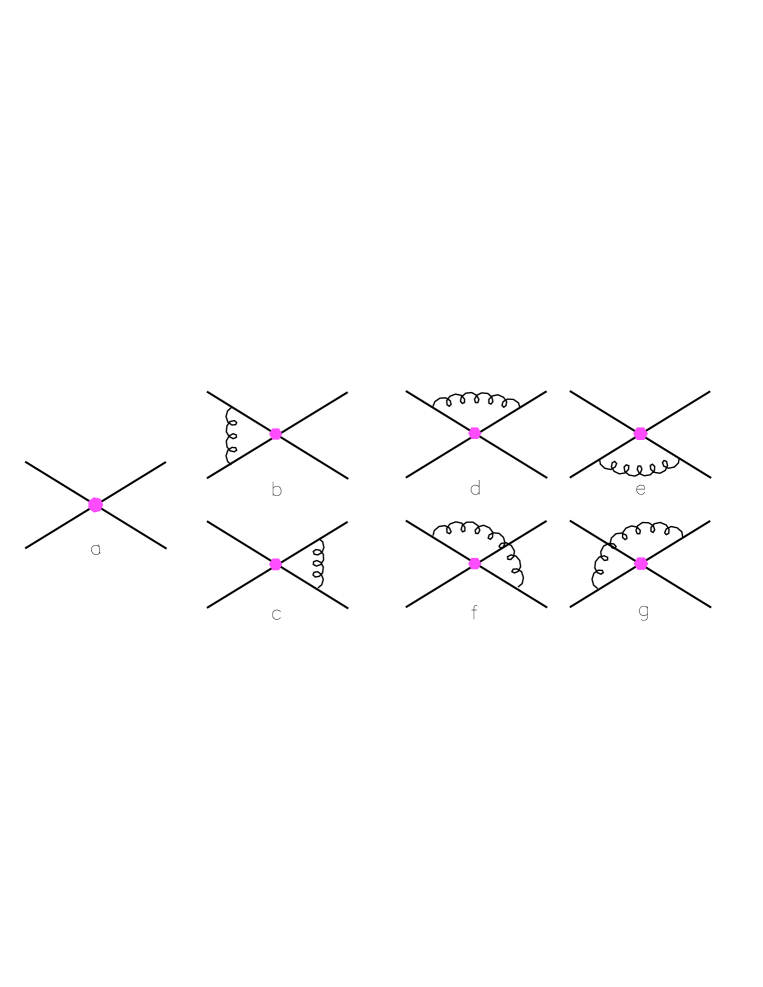
Figure 5: Diagrams for NLO corrections to the NRQCD matrix elements.

Let us first describe with some details the cancellation of the Coulomb singularity. We discuss for definiteness the case of decays, but the same applies to production cross sections. The Coulomb-singular part of the virtual correction to a two-partons decay of a ${\cal{Q}}\equiv Q\overline{Q}[\mbox{${}^{2S+1}L_{J}$}]$ state reads:

$$\hat{\Gamma}_{V}({\cal{Q}}\to ij)=\hat{\Gamma}_{\rm Born}{\mbox{$\alpha_{s}$}\over\pi}f_{\epsilon}(M^{2})\left({\cal C}{\pi^{2}\over{2v}}+\cdots\right)\,.$$ (134)

The coefficient ${\cal C}$ is a colour factor which, for ${\cal{Q}}$ in a colour-singlet or octet state, takes the value

$${\cal C}^{[1]} = {C_{F}{}}\,,$$

$${\cal C}^{[8]} = \mbox{$C_{F}-{1\over 2}C_{A}$}\,.$$ (135)

The above expression (134), multiplied by the NRQCD matrix element $\langle H|{{\cal{O}}}({\cal{Q}})|H\rangle$, provides the final answer for the virtual corrections to the decay width of the physical quarkonium state $H$. However, to get rid of the Coulomb singularity, we must first evaluate in NRQCD the radiative corrections to this matrix element. This was done for the first time in ref. [15], and we reproduce their argument for illustration.

$\langle H|{{\cal{O}}}({\cal{Q}})|H\rangle$ is depicted in fig. 5(a) in lowest order, and the higher order corrections important for the Coulomb singularities are shown in figs. 5(b,c). Let us consider, for instance, diagram 5(b).

Working in Coulomb gauge, the gluon propagator is given by the sum of a transverse part,

$$G^{\mu\nu}_{trans}(k^{2})=-{i\over k^{2}}\left(g^{\mu\nu}+{{k^{\mu}k^{\nu}}\over{{\bf k}^{2}}}\right)(1-\delta_{\mu 0})(1-\delta_{\nu 0}),$$ (136)

and of a Coulomb part,

$$G^{\mu\nu}_{Coul}(k^{2})={i\over{{\bf k}^{2}}}\delta_{\mu 0}\delta_{\nu 0}.$$ (137)

It is this second part responsible for the singularity we are looking for.

Inserting this term only and making use of NRQCD Feynman rules we get for diagram 5(b)

$$I_{b}=-ig_{s}^{2}\int{{d^{4}k}\over{(2\pi)^{4}}}{1\over{{\bf k}^{2}}}{1\over{\left[p_{0}+k_{0}-{{({\bf p}+{\bf k})^{2}}\over{2m}}+i\mbox{$\epsilon$}\right]}}\;{1\over{\left[p_{0}-k_{0}-{{({\bf p}+{\bf k})^{2}}\over{2m}}+i\mbox{$\epsilon$}\right]}}\,,$$ (138)

with the on-shell condition $p_{0}={\bf p}^{2}/2m$, $p$ being the heavy quark momentum and $k$ the gluon one. The integral over $k_{0}$ can be performed by contour integration, closing the contour in the lower half of the complex $k_{0}$ plane and picking up the pole at $k_{0}=-p_{0}+({\bf p}+{\bf k})^{2}/2m-i\mbox{$\epsilon$}$. The result is

$$I_{b}=g_{s}^{2}m\int{{d^{3}k}\over{(2\pi)^{3}}}{1\over{{\bf k}^{2}}}{1\over{{\bf k}^{2}+2{\bf p}\cdot{\bf k}-i\mbox{$\epsilon$}}}\,.$$ (139)

Being divergent, this integral must be performed within some regularization technique. Using dimensional regularization, and defining ${\bf v}={\bf p}/m$, $v=|{\bf v}|$, we find

$$I_{b}={{\pi\mbox{$\alpha_{s}$}}\over{4v}}(1+{\rm infrared~{}singular~{}imaginary~{}part})\,.$$ (140)

From the diagram 5(c) we find $I_{c}$, similar to $I_{b}$ but with opposite imaginary part. Summing the two contributions, the overall Coulomb correction to the matrix element is therefore:

$$\langle H|{{\cal{O}}}({\cal{Q}})|H\rangle=\langle H|{{\cal{O}}}({\cal{Q}})|H\rangle_{\rm Born}\left(1+{\cal C}{{\pi\mbox{$\alpha_{s}$}}\over{2v}}\right).$$ (141)

The colour factor ${\cal C}$ evaluates to the same defined above in (135), according to the operator we are correcting (the central blob in figure 5) being a colour singlet or a colour octet one.

For the decay width we have then

$$\Gamma^{H}[{\cal{Q}}\to ij] = \left(\hat{\Gamma}_{\rm Born}+\hat{\Gamma}_{V}({\cal{Q}}\to ij)+\cdots\right)\langle H|{{\cal{O}}}({\cal{Q}})|H\rangle_{\rm Born}$$ (142)

$$= \left[\hat{\Gamma}_{\rm Born}+\hat{\Gamma}_{\rm Born}{\mbox{$\alpha_{s}$}\over\pi}\left({\cal C}{\pi^{2}\over{2v}}+\cdots\right)\right]\langle H|{{\cal{O}}}({\cal{Q}})|H\rangle\left(1-{\cal C}{{\pi\mbox{$\alpha_{s}$}}\over{2v}}\right)\,.$$

Upon inspection, we can see that the singular $1/v$ terms cancel. Since no finite parts are introduced in this process, we can just drop the singular Coulomb term whenever it appears in the virtual contributions to cross sections and decay widths.

Next we consider the problem of the infrared singularity which appears for instance in the ${}^{3}P_{J}^{[1,8]}\to\mbox{$q\overline{q}$}g$ real correction process. We have mentioned in Section 4.2 how the residue of this singularity is proportional to the matrix element squared for the process ${}^{3}S_{1}^{[8]}\to\mbox{$q\overline{q}$}$, making it possible to absorb the singularity in the colour-octet wave function which accompanies this process. Again, NRQCD puts this cancellation on rigorous grounds. Radiative corrections to the colour octet matrix element $\langle H|{\cal{O}}_{8}(^{3}S_{1})|H\rangle$ display a singularity which matches the one appearing in the $P$-state decay calculation. When summing $P$-wave and ${}^{3}S_{1}$ octet processes, the singularity cancels exactly. Some finite parts are however introduced by this process, which makes it necessary to carefully evaluate the diagrams involved.

Let us then consider the radiative corrections depicted in diagrams 5(d,e,f,g). It is this time the transverse part of the gluon propagator to be relevant, and the loop integral reads

$$I_{d}=ig_{s}^{2}\int{{d^{4}k}\over{(2\pi)^{4}}}{{{\bf p}\cdot{\bf p}^{\prime}-({\bf p}\cdot{\bf k})({\bf p}^{\prime}\cdot{\bf k})/{\bf k}^{2}}\over{m^{2}(k_{0}^{2}-{\bf k}^{2}+i\mbox{$\epsilon$})}}{1\over{\left[p_{0}-k_{0}-{{({\bf p}-{\bf k})^{2}}\over{2m}}+i\mbox{$\epsilon$}\right]}}{1\over{\left[p_{0}^{\prime}-k_{0}-{{({\bf p}^{\prime}-{\bf k})^{2}}\over{2m}}+i\mbox{$\epsilon$}\right]}}\,.$$ (143)

Contour-integrating over $k_{0}$ around the $k_{0}=|{\bf k}|-i\mbox{$\epsilon$}$ pole we find

$$I_{d}=g_{s}^{2}\int{{d^{3}k}\over{(2\pi)^{3}}}{{{\bf p}\cdot{\bf p}^{\prime}-({\bf p}\cdot{\bf k})({\bf p}^{\prime}\cdot{\bf k})/{\bf k}^{2}}\over{2|{\bf k}|m^{2}}}{1\over{\left[-|{\bf k}|-{{{\bf k}^{2}}\over{2m}}+{{{\bf p}\cdot{\bf k}}\over{m}}+i\mbox{$\epsilon$}\right]}}{1\over{\left[-|{\bf k}|-{{{\bf k}^{2}}\over{2m}}+{{{\bf p}^{\prime}\cdot{\bf k}}\over{m}}+i\mbox{$\epsilon$}\right]}}\,.$$ (144)

This integral is infrared divergent but ultraviolet finite. However, it has been argued [42, 47, 19] that the correct way to perform it is to first expand [15] the integrand in powers of ${\bf p}/m$, ${\bf p}^{\prime}/m$ and ${\bf k}/m$, since it is for small values of these momenta that NRQCD is valid (though alternative approaches exist, see for instance ref. [48]). Such an expansion produces

$$I_{d}={{g_{s}^{2}}\over{2m^{2}}}\int{{d^{3}k}\over{(2\pi)^{3}}}{{{\bf p}\cdot{\bf p}^{\prime}-({\bf p}\cdot{\bf k})({\bf p}^{\prime}\cdot{\bf k})/{\bf k}^{2}}\over{|{\bf k}|^{3}}}\,,$$ (145)

which is now both infrared and ultraviolet divergent. We can perform it by using dimensional regularization and obtain

$$I_{d}={{4\pi\mbox{$\alpha_{s}^{(b)}$}}\over{2m^{2}}}{{{\bf p}\cdot{\bf p}^{\prime}}\over{3\pi^{2}}}{1\over 2}\left({1\over\mbox{$\epsilon_{\!\!\mbox{ \tiny{UV} }}$}}-{1\over\mbox{$\epsilon_{\!\!\mbox{ \tiny{IR} }}$}}\right)\,,$$ (146)

where $\epsilon_{\!\!\mbox{ \tiny{IR} }}$ and $\epsilon_{\!\!\mbox{ \tiny{UV} }}$ are poles of infrared and ultraviolet origin respectively. It is to be noted that this ultraviolet divergence arises within NRQCD, and has nothing to do with the ultraviolet divergences which appear in the virtual corrections within full QCD, to be subsequently removed by renormalization of the coupling constant.

The other three diagrams give identical result but with different colour factors when including the colour structure of the ${\cal{O}}_{8}(^{3}S_{1})$ operator we are correcting. Using eqs. (350,351) we get for the sum of the four diagrams

$$I={{4\mbox{$\alpha_{s}^{(b)}$}}\over{3\pi m^{2}}}\left({1\over\mbox{$\epsilon_{\!\!\mbox{ \tiny{UV} }}$}}-{1\over\mbox{$\epsilon_{\!\!\mbox{ \tiny{IR} }}$}}\right){\cal{O}}_{8}(^{3}S_{1})\left[{C_{F}{}}{1\otimes 1\over 2{N_{c}{}}}+{B_{F}{}}T^{a}\otimes T^{a}\right]{\bf p}\cdot{\bf p}^{\prime}\,.$$ (147)

The diagrams depicted in fig. 5 formally describe annihilation matrix elements $\langle H|{\cal{O}}({\cal{Q}})|H\rangle$, but the result is identical for the production ones $\langle{\cal{O}}^{H}({\cal{Q}})\rangle$. Recalling the definition of ${\cal{O}}_{[1,8]}(^{3}P_{J})$ (see Appendix A) we can write

$$\langle H|{\cal{O}}_{8}(^{3}S_{1})|H\rangle = \langle H|{\cal{O}}_{8}(^{3}S_{1})|H\rangle_{\rm Born}+{{4\mbox{$\alpha_{s}^{(b)}$}}\over{3\pi m^{2}}}\left({1\over\mbox{$\epsilon_{\!\!\mbox{ \tiny{UV} }}$}}-{1\over\mbox{$\epsilon_{\!\!\mbox{ \tiny{IR} }}$}}\right)$$ (148)

$$\times\left[{C_{F}{}}\sum_{J=0}^{2}\langle H|{\cal{O}}_{1}(^{3}P_{J})|H\rangle+{B_{F}{}}\sum_{J=0}^{2}\langle H|{\cal{O}}_{8}(^{3}P_{J})|H\rangle\right]\,.$$

The presence of the ultraviolet singularity indicates that the $\langle H|{\cal{O}}_{8}(^{3}S_{1})|H\rangle$ operator needs renormalization. The suitable counterterm in the ${\overline{\rm MS}}$ scheme is such that the relation between the bare ($D$-dimensional) and the renormalized matrix element reads

$$\langle H|{\cal{O}}_{8}(^{3}S_{1})|H\rangle = {\mu_{\Lambda}}^{-2\mbox{$\epsilon$}}\left\{\langle H|{\cal{O}}_{8}(^{3}S_{1})|H\rangle^{({\mu_{\Lambda}})}+{{4\mbox{$\alpha_{s}$}}\over{3\pi m^{2}}}\left({1\over\mbox{$\epsilon_{\!\!\mbox{ \tiny{UV} }}$}}+\ln 4\pi-\gamma_{E}\right)\right.$$ (149)

$$\times\left.\left[{C_{F}{}}\sum_{J=0}^{2}\langle H|{\cal{O}}_{1}(^{3}P_{J})|H\rangle+{B_{F}{}}\sum_{J=0}^{2}\langle H|{\cal{O}}_{8}(^{3}P_{J})|H\rangle\right]\right\},$$

${\mu_{\Lambda}}$ being the NRQCD renormalization scale. Since the renormalized matrix elements on the right hand side have mass dimension three while the bare $D$-dimensional one on the left has dimension $D-1$ (a factor of $2(D-1)$ coming from the four spinor fields of the operator plus a factor of $-(D-1)$ from the nonrelativistic normalization of the $|H\rangle$ states, $\langle H({\bf p})|H({\bf p^{\prime}})\rangle=(2\pi)^{D-1}\delta^{D-1}({\bf p}-{\bf p^{\prime}})$), the ${\mu_{\Lambda}}^{-2\mbox{$\epsilon$}}$ compensates for the difference.

Using eqs.(148,149) (no renormalization is necessary at this order for the $\langle H|{\cal{O}}_{[1,8]}(^{3}P_{J})|H\rangle$ matrix elements) we find

$$\langle H|{\cal{O}}_{8}(^{3}S_{1})|H\rangle_{\rm Born} = {\mu_{\Lambda}}^{-2\mbox{$\epsilon$}}\langle H|{\cal{O}}_{8}(^{3}S_{1})|H\rangle^{({\mu_{\Lambda}})}+\left({1\over\mbox{$\epsilon_{\!\!\mbox{ \tiny{IR} }}$}}+\ln 4\pi-\gamma_{E}\right)\left({\mu\over{\mu_{\Lambda}}}\right)^{2\mbox{$\epsilon$}}{{4\mbox{$\alpha_{s}$}}\over{3\pi m^{2}}}$$ (150)

$$\times\left[{C_{F}{}}\sum_{J=0}^{2}\langle H|{\cal{O}}_{1}(^{3}P_{J})|H\rangle+{B_{F}{}}\sum_{J=0}^{2}\langle H|{\cal{O}}_{8}(^{3}P_{J})|H\rangle\right]\,.$$

This equation can now be used to cancel the infrared pole in the ${{}^{3}P_{J}}\to\mbox{$q\overline{q}$}g$ processes given in eqs. (116, 120): summing to these decays the colour-octet one ${{}^{3}S_{1}}^{[8]}\to\mbox{$q\overline{q}$}$ and substituting the bare matrix element with the expression given above one finds (restricting ourselves to the infrared singular parts):

$$\sum_{J}\Gamma^{H}(\mbox{${}^{3}P_{J}^{[1]}$}\to\mbox{$q\overline{q}$}g)+\Gamma^{H}({{}^{3}S_{1}}^{[8]}\to\mbox{$q\overline{q}$})=$$ (151)

$$= \sum_{J}\left\{-{4\over 9}{n_{f}{}}{C_{F}{}}\mbox{$\alpha_{s}^{3}$}{\mu^{2\mbox{$\epsilon$}}\langle H|{\cal{O}}_{1}(^{3}P_{J})|H\rangle\over m^{4}}\left[{1\over\mbox{$\epsilon_{\!\!\mbox{ \tiny{IR} }}$}}{f_{\epsilon}(M^{2})\over K}\left({4\pi\mu^{2}\over M^{2}}\right)^{\epsilon}{\Gamma(1-\epsilon)\over\Gamma(2-2\epsilon)}+a_{J}\right]+\mbox{ IR-finite}\right\}$$

$$+{{\mbox{$\alpha_{s}^{2}$}\pi}\over{m^{2}}}\left({{4\pi\mu^{2}}\over{4m^{2}}}\right)^{\epsilon}{{\Gamma(1-\mbox{$\epsilon$})}\over{\Gamma(2-2\mbox{$\epsilon$})}}{{(1-\mbox{$\epsilon$})}\over{(3-2\mbox{$\epsilon$})}}$$

$$\times\left({1\over\mbox{$\epsilon_{\!\!\mbox{ \tiny{IR} }}$}}+\ln 4\pi-\gamma_{E}\right)\left({\mu\over{\mu_{\Lambda}}}\right)^{2\epsilon}{{4\mbox{$\alpha_{s}$}}\over{3\pi m^{2}}}{n_{f}{}}{C_{F}{}}\mu^{2\epsilon}\sum_{J}\langle H|{\cal{O}}_{1}(^{3}P_{J})|H\rangle+\mbox{ IR-finite}$$

$$= \sum_{J}\left\{-{4\over 9}{C_{F}{}}\mbox{$\alpha_{s}^{3}$}{\langle H|{\cal{O}}_{1}(^{3}P_{J})|H\rangle\over m^{4}}\left[a_{J}+{1\over 3}+\log{{\mu_{\Lambda}}^{2}\over 4m^{2}}\right]+\cdots\right\}$$

7 Production processes

7.1 Kinematics and factorization of soft and collinear singularities

The technique used to extract the soft and collinear singularities from the real emission processes is similar to the one employed in the study of decays. The kinematics of the process $k_{1}+k_{2}\to P+k_{3}$, where $P$ is the momentum of the heavy quark pair ( identified by ${\cal{Q}}^{[1,8]}$ ) and $k_{i}$ are the momenta of the massless partons, can be described in terms of the standard Mandelstam variables $s$, $t$ and $u$, defined by

$$s = (k_{1}+k_{2})^{2}\;,$$ (152)

$$t = (k_{2}-k_{3})^{2}\;\equiv\;-{s\over 2}(1-x)(1-y)\;,$$ (153)

$$u = (k_{1}-k_{3})^{2}\;\equiv\;-{s\over 2}(1-x)(1+y)\;.$$ (154)

Here we also have introduced the Lorentz invariant dimensionless variables $x=4m^{2}/s$ and $y$ ($-1<y<1$), defined by the above equations. In the center-of-mass frame of the partonic collisions, the variable $y$ becomes the cosine of the scattering angle $\theta$. In terms of $x$ and $y$ the total partonic cross section can be written in $D$ dimensions as follows:

$$\sigma\;=\;{1\over 2s}\int d\Phi_{(2)}(x,y)\;\mbox{${\cal{M}}$}(x,y)\;,$$ (155)

where $\mbox{${\cal{M}}$}=\overline{\sum}|A|^{2}$ is the spin- and colour-averaged matrix element squared in $D$ dimensions and $d\Phi_{(2)}(x,y)$ is the $D$-dimensional two-body phase space:

$$d\Phi_{(2)}(x,y)\;=\;{4^{\epsilon}\over K}\,\left({4\pi\over s}\right)^{\epsilon}\,\Gamma(1+\epsilon)\,{1\over 16\pi}\,(1-x)^{1-2\epsilon}\,(1-y^{2})^{-\epsilon}\,dy\;.$$ (156)

The soft and collinear singularities are associated to the vanishing of $t$ or $u$, which appear at most as single poles in the expression of ${\cal{M}}$. One can therefore introduce the finite, rescaled amplitude squared ${\overline{\cal{M}}}$:

$$\mbox{${\cal{M}}$}\;=\;{1\over ut}\,\mbox{${\overline{\cal{M}}}$}\;=\;{4\over s^{2}(1-x)^{2}(1-y^{2})}\,\mbox{${\overline{\cal{M}}}$}\;.$$ (157)

In terms of ${\overline{\cal{M}}}$, the partonic cross section reads as follows:

$$\sigma(x)\;=\;{4C\over s^{2}}\,(1-x)^{-1-2\epsilon}\,\int_{-1}^{1}\,dy\,(1-y^{2})^{-1-\epsilon}\,\mbox{${\overline{\cal{M}}}$}(x,y)\,dy\;,$$ (158)

$$C\;=\;{4^{\epsilon}\over K}\,\left({4\pi\over s}\right)^{\epsilon}\,\Gamma(1+\epsilon)\,{1\over 32\pi s}\;.$$ (159)

As in the case of decays, soft and collinear singularities are now all exhibited by the universal poles which develop as $x\to 1$ and $y^{2}\to 1$. The residues of these poles can be derived without an explicit calculation of the matrix elements, as they only depend on the universal structure of collinear and soft singularities. We will carry out an explicit evaluation of these residues in the case of colour-singlet production in the $gg\to{\cal{Q}}^{[1]}g$ process in the next subsection. The other cases are similar, and will be discussed with fewer details in the following.

7.1.1 $gg\to g{\cal{Q}}^{[1]}$ processes

Figure 6: Diagrams for the real corrections to the $gg$ channels. Permutations of outgoing gluons and/or reversal of fermion lines are always implied.

We start by considering the soft limit, $x\to 1$. The following distributional identity holds for small $\epsilon$:

$$(1-x)^{-1-2\epsilon}\;=\;-{\beta^{-4\epsilon}\over 2\epsilon}\delta(1-x)+\left({1\over 1-x}\right)_{\rho}\,-\,2\epsilon\left({\log(1-x)\over 1-x}\right)_{\rho}\,+\,{\cal{O}}(\epsilon^{2})\,$$ (160)

where $\rho=M^{2}/S_{had}$, $\beta=\sqrt{1-\rho}$, and the $\rho$-distributions are defined by:

$$\int_{\rho}^{1}\,dx\;\left[d(x)\right]_{\rho}t(x)\;=\;\int_{\rho}^{1}\,dx\;d(x)\;\left[t(x)-t(1)\right]\;.$$ (161)

We can therefore write, with obvious notation,

$$\sigma(x)\;=\;\sigma_{x=1}+\sigma_{x\neq 1}\;.$$ (162)

The first terms on the right-hand side is given by the following expression:

$$\sigma_{x=1}\;=\;-{4C\over M^{4}}\,{\beta^{-4\epsilon}\over 2\epsilon}\,\delta(1-x)\,\int_{-1}^{1}\,dy\,(1-y^{2})^{-1-\epsilon}\,\mbox{${\overline{\cal{M}}}$}(x=1,y)\;,\\$$ (163)

The $x\to 1$ limit of ${\overline{\cal{M}}}$ can be easily derived from eq.(48):

$$\mbox{${\cal{M}}$}(x,y) \stackrel{{\scriptstyle x\to 1}}{{\longrightarrow}} g^{2}\,{C_{A}{}}\,{4s\over ut}\,\mbox{${\cal{M}}_{\rm Born}$}\,$$ (164)

$$\mbox{${\overline{\cal{M}}}$}(x,y) \stackrel{{\scriptstyle x\to 1}}{{\longrightarrow}} 4s\,g^{2}\,{C_{A}{}}\,\mbox{${\cal{M}}_{\rm Born}$}\;,$$ (165)

where ${\cal{M}}_{\rm Born}$ is the $D$-dimensional Born amplitude squared for the $gg\to{\cal{Q}}$ process, which is independent of $y$. The integration over $y$ of eq.(163) is elementary, and leads to the following result:

$$\sigma_{x=1}\;=\;{f_{\epsilon}(s)\over\epsilon^{2}}\,H\,{C_{A}{}}\,{\mbox{$\alpha_{s}$}\over\pi}\beta^{-4\epsilon}\,\mbox{$\sigma_{\rm Born}$}\;,$$ (166)

where $H$ is defined by

$$H\;=\;{\Gamma(1-\epsilon)\over\Gamma(1+\epsilon)\Gamma(1-2\epsilon)}\;=\;1-{\pi^{2}\over 3}\epsilon^{2}+{\cal O}(\epsilon^{3})\;,$$ (167)

and $\sigma_{\rm Born}$ is the $D$-dimensional Born cross section:

$$\mbox{$\sigma_{\rm Born}$}\;=\;{\pi\over M^{4}}\;\mbox{${\cal{M}}_{\rm Born}$}\;\delta(1-x)\;\equiv\;\mbox{$\sigma_{0}$}\delta(1-x)\;.$$ (168)

The collinear singularities remaining in $\sigma_{x\neq 1}$ can be factored out by using the following distributional identity:

$$(1-y^{2})^{-1-\epsilon} = -\left[\delta(1-y)+\delta(1+y)\right]{4^{-\epsilon}\over 2\epsilon}$$ (169)

$$+{1\over 2}\left[\left({1\over 1-y}\right)_{+}+\left({1\over 1+y}\right)_{+}\right]+{\cal O}(\epsilon)\;,$$

where the distributions on the right-hand side are defined by:

$$\int_{-1}^{1}\,dy\,\left({1\over 1\pm y}\right)_{+}t(y)\;=\;\int_{-1}^{1}\,dy\,{1\over 1\pm y}\left[t(y)-t(\mp 1)\right]\;.$$ (170)

The contribution $\sigma_{x\neq 1}$ can then be split into three terms:

$$\sigma_{x\neq 1}\;=\;\sigma_{y=1}+\sigma_{y=-1}+\sigma_{\rm finite}\;.$$ (171)

The term $\sigma_{\rm finite}$ has no residual divergences, and is given by the following expression:

$$\sigma_{\rm finite}\;=\;{2C\over s^{2}}\left({1\over 1-x}\right)_{\rho}\,\int_{-1}^{1}\,dy\,\left[\left({1\over 1-y}\right)_{+}+\left({1\over 1+y}\right)_{+}\right]\,\mbox{${\overline{\cal{M}}}$}(x,y)\;.$$ (172)

This piece explicitly depends on the nature of the quarkonium state produced. For processes whose Born contribution vanishes, this is the only non zero term.

The remaining pieces, $\sigma_{y=\pm 1}$, are given by:

$$\sigma_{y=\pm 1}\;=\;-{4C\over s^{2}}\,{4^{-\epsilon}\over 2\epsilon}\,\left[\left({1\over 1-x}\right)_{\rho}-2\epsilon\left({\log(1-x)\over 1-x}\right)_{\rho}\right]\,\mbox{${\overline{\cal{M}}}$}(x,y=\pm 1)\;.$$ (173)

The limits for $y\to\pm 1$ of $\mbox{${\overline{\cal{M}}}$}(x,y)$ are universal, thanks to the factorization of collinear singularities:

$$\mbox{${\overline{\cal{M}}}$}(x,y)\stackrel{{\scriptstyle y\to\pm 1}}{{\longrightarrow}}8\pi\,s\,\mbox{$\alpha_{s}^{(b)}$}P_{gg}(x){1-x\over x}\mbox{${\cal{M}}_{\rm Born}$}\;,$$ (174)

where $P_{gg}(x)$ is the standard $D=4$ Altarelli-Parisi splitting kernel, defined in Appendix A. Using these relations we get:

$$\sigma_{y=\pm 1}\;=\;-{1\over\bar{\epsilon}}\,\left({\mu^{2}\over s}\right)^{\epsilon}\,{\mbox{$\alpha_{s}$}\over 2\pi}\,P_{gg}(x)\,(1-x)x\,\mbox{$\sigma_{0}$}\,\left[\left({1\over 1-x}\right)_{\rho}-2\epsilon\left({\log(1-x)\over 1-x}\right)_{\rho}\right]\;,$$ (175)

where

$${1\over\bar{\epsilon}}\;=\;{1\over\epsilon}-\gamma_{\rm E}+\log(4\pi)\;,$$ (176)

The collinear poles take the form dictated by the factorization theorem. According to this the parton cross section can be written as:

$${\rm d}\sigma_{ij}(p_{1},p_{2}) = \sum_{k,l}{\rm d}\hat{\sigma}_{kl}(x_{1}p_{1},x_{2}p_{2})\Gamma_{ki}(x_{1})\Gamma_{lj}(x_{2}){\rm d}x_{1}{\rm d}x_{2}\;,$$ (177)

$$\Gamma_{ij}(x) = \delta_{ij}\delta(1-x)\;-\;{1\over\bar{\epsilon}}\,{\mbox{$\alpha_{s}$}\over 2\pi}\left({\mu^{2}\over\mbox{$\mu^{2}_{\rm F}$}}\right)^{\epsilon}{\cal P}_{ij}(x)\;+\;K_{ij}(x)\;,$$ (178)

where ${\rm d}\hat{\sigma}$ is free of collinear singularities as $\epsilon\to 0$. Here we allowed the factorization scale $\mu_{\rm F}$ to differ from the renormalization scale $\mu$. The functions ${\cal P}_{ij}(x)$ are the $D=4$ Altarelli-Parisi splitting kernels, collected in Appendix A, and the factors $K_{ij}$ are arbitrary functions, defining the factorization scheme. In this paper we adopt the $\overline{\rm MS}$  factorization, in which $K_{ij}(x)=0$ for all $i,j$. For the definition of $K_{ij}(x)$ in the DIS scheme, see for example ref. [37]. The collinear factors $\Gamma(x)$ are usually reabsorbed into the hadronic parton densities, and the physical cross section is then expressed as:

$${\rm d}\sigma_{H_{1}H_{2}}(p_{1},p_{2})\;=\;\sum_{k,l}{\rm d}\hat{\sigma}_{kl}(x_{1}p_{1},x_{2}p_{2},\mbox{$\mu_{\rm F}$})F_{kH_{1}}(x_{1},\mbox{$\mu_{\rm F}$})F_{lH_{2}}(x_{2},\mbox{$\mu_{\rm F}$}){\rm d}x_{1}{\rm d}x_{2}\;,$$ (179)

where $F_{kH}(x,\mbox{$\mu_{\rm F}$})$ is the density of the parton $k$ in the hadron $H$, evaluated at the factorization scale $\mu_{\rm F}$. Expanding eq. (177) order by order in $\alpha_{s}$, we extract the following counter-terms $\sigma^{(c)}_{y=\pm 1}$: defined by

$$\sigma^{(c)}_{y=\pm 1}\;=\;{1\over\bar{\epsilon}}\,{\mbox{$\alpha_{s}$}\over 2\pi}\left({\mu^{2}\over\mbox{$\mu^{2}_{\rm F}$}}\right)^{\epsilon}\,{\cal{P}}_{gg}({x}\,)x\mbox{$\sigma_{0}$}\;,$$ (180)

with

$${\cal P}_{gg}(x)=2{C_{A}{}}\left[{x\over(1-x)_{\rho}}+{1-x\over x}+x(1-x)\right]+\left(\mbox{$b_{0}$}+4{C_{A}{}}\log\beta\right)\delta(1-x)\,.$$ (181)

Putting together all pieces, we come to the final result for the real emission cross section:

$$\sigma^{H}[g\,g\to{\cal{Q}}^{[1]}\,g] = {\mbox{$\alpha_{s}$}\over\pi}\sigma_{0}^{H}[gg\to{\cal{Q}}^{[1]}]$$ (182)

$$\times\left\{f_{\epsilon}(s)\left[{C_{A}{}}\left({1\over\mbox{$\epsilon$}^{2}}+{11\over 6\mbox{$\epsilon$}}-{\pi^{2}\over 3}+8\log^{2}\beta\right)-{2\over 3\mbox{$\epsilon$}}{n_{f}{}}{T_{F}{}}\right]\delta(1-x)\right.$$

$$+\left.\left[x{\cal P}_{gg}(x)\log{s\over\mbox{$\mu^{2}_{\rm F}$}}+2x(1-x)P_{gg}(x)\left({\log(1-x)\over 1-x}\right)_{\rho}\right.\right.$$

$$+\left.\left.\left({1\over 1-x}\right)_{\rho}f_{gg}[{\cal{Q}}^{[1]}](x)\right]\right\},\quad\,\quad$$

$$[{\cal{Q}}^{[1]}=\mbox{${}^{1}S_{0}^{[1]}$},\mbox{${}^{3}P_{0}^{[1]}$},\mbox{${}^{3}P_{2}^{[1]}$}]\;,$$

where $\sigma_{0}^{H}[gg\to{\cal{Q}}^{[1]}]$ is the $D$-dimensional, Born-level partonic cross section for the production of the quarkonium state $H$ via the ${\cal{Q}}^{[1]}$ intermediate state, after removal of the $\delta(1-x)$ term (see eq. (168)). The finite functions $f_{gg}(x)$, obtained from the explicit evaluation of eq. (172), are collected in Appendix C.

The result for the ${}^{1}S_{0}^{[1]}$ state agrees with previous calculations [37, 7]. The results for the $P$ waves are new. In the case of ${{}^{3}S_{1}}$ and ${{}^{3}P_{1}}$ production the $O(\alpha_{s}^{3})$ process is the leading order one. Integration over the emitted gluon phase space is completely finite, and the results have been known for long time in the literature (see e.g. ref. [7]). For completeness, we collect them in Appendix C.

7.1.2 $qg\to q{\cal{Q}}^{[1]}$ processes

The Born level processes $qg\to{\cal{Q}}^{[1]}$ identically vanish. As a result no IR divergence is present at $O(\alpha_{s}^{3})$ and virtual corrections are not present. The only singularities appearing at this order come from the emission of the final-state quark collinear to the initial-state one. The behaviour of the amplitude in the $y\to 1$ collinear limit is again controlled by the Altarelli-Parisi splitting functions:

$$\mbox{${\overline{\cal{M}}}$}(x,y)\stackrel{{\scriptstyle y\to 1}}{{\longrightarrow}}8\pi\,s\,\mbox{$\alpha_{s}^{(b)}$}P_{gq}(x){1-x\over x}\mbox{${\cal{M}}_{\rm Born}$}\;.$$ (183)

In analogy to the $gg$ case, one introduces the following counter-term in the $\overline{\rm MS}$  scheme:

$$\sigma^{(c)}_{y=1}\;=\;{1\over\bar{\epsilon}}\,{\mbox{$\alpha_{s}$}\over 2\pi}\left({\mu^{2}\over\mbox{$\mu^{2}_{\rm F}$}}\right)^{\epsilon}\,{\cal{P}}_{gq}({x}\,)x\mbox{$\sigma_{0}$}\;,$$ (184)

where ${\cal{P}}_{gq}({x}$ is)defined in Appendix A.

Following a procedure analogous to the one detailed in the case of $gg$ production, we find the following result:

$$\sigma^{H}[g\,q\to{\cal{Q}}^{[1]}\,q] = {\mbox{$\alpha_{s}$}\over\pi}\sigma_{0}^{H}[gg\to{\cal{Q}}^{[1]}]$$ (185)

$$\times\left\{\left[{x\over 2}{\cal P}_{gq}(x)\log{s(1-x)^{2}\over\mbox{$\mu^{2}_{\rm F}$}}+{C_{F}{}}{x^{2}\over 2}\right]+f_{gq}[{\cal{Q}}^{[1]}](x)\right\}\,,$$

$$[{\cal{Q}}^{[1]}=\mbox{${}^{1}S_{0}^{[1]}$},\mbox{${}^{3}P_{0}^{[1]}$},\mbox{${}^{3}P_{2}^{[1]}$}]\;,$$

where the functions $f_{gq}(x)$ are collected in Appendix C, together with the result for ${{}^{3}P_{1}}^{[1]}$ production, for which no collinear singularity is present to start with. Our result for ${}^{1}S_{0}^{[1]}$ production agrees with those presented in refs. [37, 7]. In the case of ${{}^{3}P_{0}}^{[1]}$ and ${{}^{3}P_{2}}^{[1]}$ we differ from ref. [7] by the factor ${C_{F}{}}x^{2}/2$ in eq.(185). This piece arises from the $\overline{\rm MS}$  factorization prescription, which dictates use of the $D=4$ Altarelli-Parisi kernel in the collinear counter-term, eq. (184).

7.1.3 $\mbox{$q\overline{q}$}\to g{\cal{Q}}^{[1]}$ processes

In this case no collinear divergences are present upon integration over the final-parton phase space. No virtual corrections are present either. Infrared divergences however appear, associated to the presence of an intermediate ${}^{3}S_{1}^{[8]}$ state:

$$\sigma^{H}[\mbox{$q\overline{q}$}\to\mbox{${}^{3}P_{J}^{[1]}$}\,g] = -{{C_{F}{}}\over D_{F}^{2}}{256\pi^{2}\mbox{$\alpha_{s}^{3}$}\mu^{4\mbox{$\epsilon$}}\over 9{(2m)}^{7}}\beta^{-4\mbox{$\epsilon$}}f_{\epsilon}(s)\left({1\over\mbox{$\epsilon$}}+{4\over 3}\right)\delta(1-x)\langle{\cal{O}}^{H}_{1}({{}^{3}P_{J}})\rangle$$ (186)

$$+{\pi^{2}\mbox{$\alpha_{s}^{3}$}\mu^{4\mbox{$\epsilon$}}\over{(2m)}^{7}}\left({1\over 1-x}\right)_{\rho}f_{\tiny\mbox{$q\overline{q}$}}[\mbox{${}^{3}P_{J}^{[1]}$}](x)\langle{\cal{O}}^{H}_{1}({{}^{3}P_{J}})\rangle\qquad[J=0,1,2]\,,$$

where ${D_{F}{}}$ is defined in Appendix A. The infrared divergences is absorbed by the inclusion of the $\mbox{$q\overline{q}$}\to{}^{3}S_{1}^{[8]}$ process, as discussed in Section 6. The resulting finite expressions and the functions $f_{qq}(x)$, as well as the trivial result for the ${}^{1}S_{0}^{[1]}$ production, are collected in Appendix C.

7.1.4 $gg\to g{\cal{Q}}^{[8]}$ processes

The diagrams of fig. 6 have been evaluated in 4-dimensions for colour-octet production in ref. [24]. Since the Born cross sections $gg\to{\cal{Q}}^{[8]}$ do not all vanish we expect both infrared and collinear singularities to appear. After subtraction of the collinear poles in the $\overline{MS}$ scheme the partonic cross sections read

$$\mbox{$\sigma^{H}$}[g\,g\to\mbox{${}^{3}S_{1}^{[8]}$}\,g] = {\mbox{$\alpha_{s}^{3}$}\pi^{2}\over{(2m)}^{5}}f_{gg}[\mbox{${}^{3}S_{1}^{[8]}$}](x)\langle{\cal{O}}^{H}_{8}(^{3}S_{1})\rangle$$ (187)

$$\mbox{$\sigma^{H}$}[g\,g\to\mbox{${}^{3}P_{1}^{[8]}$}\,g] = {\mbox{$\alpha_{s}^{3}$}\pi^{2}\over{(2m)}^{7}}f_{gg}[\mbox{${}^{3}P_{1}^{[8]}$}](x)\langle{\cal{O}}^{H}_{8}(^{3}P_{1})\rangle$$ (188)

$$\mbox{$\sigma^{H}$}[g\,g\to{\cal{Q}}^{[8]}\,g] = {\mbox{$\alpha_{s}$}\over\pi}\mbox{$\sigma_{0}^{H}$}[gg\to{\cal{Q}}^{[8]}]$$ (189)

$$\times\left\{f_{\epsilon}(s)\left[{C_{A}{}}\left({1\over\mbox{$\epsilon$}^{2}}+{7\over 3\mbox{$\epsilon$}}+1-{\pi^{2}\over 3}-2\log\beta+8\log^{2}\beta\right)-{2\over 3\mbox{$\epsilon$}}{n_{f}{}}{T_{F}{}}\right]\delta(1-x)\right.$$

$$+\left.\left[x{\cal P}_{gg}(x)\log{s\over\mbox{$\mu^{2}_{\rm F}$}}+2x(1-x)P_{gg}(x)\left({\log(1-x)\over 1-x}\right)_{\rho}\right.\right.$$

$$+\left.\left.\left({1\over 1-x}\right)_{\rho}f_{gg}[{\cal{Q}}^{[8]}](x)\right]\right\}\,,$$

$$[{\cal{Q}}^{[8]}=\mbox{${}^{1}S_{0}^{[8]}$},\mbox{${}^{3}P_{0}^{[8]}$},\mbox{${}^{3}P_{2}^{[8]}$}]\,,$$

with the functions $f_{gg}[{\cal{Q}}^{[8]}](x)$ collected in Appendix C.

7.1.5 $qg\to q{\cal{Q}}^{[8]}$ processes

These processes proceed via the diagrams of fig. 7. Diagrams b) and c) only contribute to ${}^{3}S_{1}^{[8]}$ production.

Figure 7: Diagrams for the $gq$ channels. Reversal of fermion lines is always implied.

Since no ${\cal O}(\mbox{$\alpha_{s}^{2}$})$ cross sections exist for these channels the results are expected to be infrared finite, only collinear singularities being allowed as long as $gg\to{\cal{Q}}^{[8]}$ is non vanishing. Notice the special case of ${}^{3}S_{1}^{[8]}$ production, whose collinear singularity is rather subtracted by the $\mbox{$q\overline{q}$}\to\mbox{${}^{3}S_{1}^{[8]}$}$ Born term.

The cross sections read:

$$\mbox{$\sigma^{H}$}[g\,q\to\mbox{${}^{3}S_{1}^{[8]}$}\,q] = {\mbox{$\alpha_{s}$}\over\pi}\mbox{$\sigma_{0}^{H}$}[\mbox{$q\overline{q}$}\to\mbox{${}^{3}S_{1}^{[8]}$}]$$ (190)

$$\times\left\{\left[{x\over 2}{\cal P}_{qg}(x)\log{s(1-x)^{2}\over\mbox{$\mu^{2}_{\rm F}$}}+{T_{F}{}}x^{2}(1-x)\right]+f_{gq}[\mbox{${}^{3}S_{1}^{[8]}$}](x)\right\}$$

$$\mbox{$\sigma^{H}$}[g\,q\to\mbox{${}^{3}P_{1}^{[8]}$}\,q] = {\pi^{2}\mbox{$\alpha_{s}^{3}$}\over{(2m)}^{7}}f_{gq}[\mbox{${}^{3}P_{1}^{[8]}$}](x)\langle{\cal{O}}^{H}_{8}(^{3}P_{1})\rangle$$ (191)

$$\mbox{$\sigma^{H}$}[g\,q\to{\cal{Q}}^{[8]}\,q] = {\mbox{$\alpha_{s}$}\over\pi}\mbox{$\sigma_{0}^{H}$}[gg\to{\cal{Q}}^{[8]}]$$

$$\times\left\{\left[{x\over 2}{\cal P}_{gq}(x)\log{s(1-x)^{2}\over\mbox{$\mu^{2}_{\rm F}$}}+{C_{F}{}}{x^{2}\over 2}\right]+f_{gq}[{\cal{Q}}^{[8]}](x)\right\}$$

$$[{\cal{Q}}^{[8]}=\mbox{${}^{1}S_{0}^{[8]}$},\mbox{${}^{3}P_{0}^{[8]}$},\mbox{${}^{3}P_{2}^{[8]}$}]$$

7.1.6 $\mbox{$q\overline{q}$}\to g{\cal{Q}}^{[8]}$ processes

Figure 8: Diagrams for the real corrections to the $q\overline{q}$ channels. Permutations of outgoing gluons and/or reversal of fermion lines are always implied.

The diagrams for these channels are depicted in fig. 8. After subtraction of the collinear singularities the cross sections read

$$\mbox{$\sigma^{H}$}[\mbox{$q\overline{q}$}\to\mbox{${}^{3}S_{1}^{[8]}$}\,g] = {\mbox{$\alpha_{s}$}\mu^{2\mbox{$\epsilon$}}\over\pi}\mbox{$\sigma_{0}^{H}$}[\mbox{$q\overline{q}$}\to\mbox{${}^{3}S_{1}^{[8]}$}]\times\left\{f_{\epsilon}(s)\left[{C_{F}{}}\left({1\over\mbox{$\epsilon$}^{2}}+{3\over 2\mbox{$\epsilon$}}-{\pi^{2}\over 3}+8\log^{2}\beta\right)\right.\right.$$ (193)

$$+\left.\left.{C_{A}{}}\left({1\over 2\mbox{$\epsilon$}}+1-2\log\beta\right)\right]\delta(1-x)\right.$$

$$+\left[x{\cal P}_{qq}(x)\log{s\over\mbox{$\mu^{2}_{\rm F}$}}+{C_{F}{}}x(1-x)+2x(1-x)P_{qq}(x)\left({\log(1-x)\over 1-x}\right)_{\rho}\right]$$

$$+\left.\left({1\over 1-x}\right)_{\rho}f_{\tiny\mbox{$q\overline{q}$}}[\mbox{${}^{3}S_{1}^{[8]}$}](x)\right\}$$

$$\mbox{$\sigma^{H}$}[\mbox{$q\overline{q}$}\to\mbox{${}^{3}P_{J}^{[8]}$}\,g] = -{{B_{F}{}}\over D_{F}^{2}}{256\pi^{2}\mbox{$\alpha_{s}^{3}$}\mu^{6\mbox{$\epsilon$}}\over 9{(2m)}^{7}}\beta^{-4\mbox{$\epsilon$}}f_{\epsilon}(s)\left({1\over\mbox{$\epsilon$}}+{4\over 3}\right)\delta(1-x)\langle{\cal{O}}^{H}_{8}(^{3}P_{J})\rangle$$ (194)

$$+{\pi^{2}\mbox{$\alpha_{s}^{3}$}\over{(2m)}^{7}}\left({1\over 1-x}\right)_{\rho}f_{\tiny\mbox{$q\overline{q}$}}[\mbox{${}^{3}P_{J}^{[8]}$}](x)\langle{\cal{O}}^{H}_{8}(^{3}P_{J})\rangle\qquad[J=0,1,2]\,,$$

and ${B_{F}{}}$ and ${D_{F}{}}$ are defined in Appendix A.

A few comments are in order.

The production of ${}^{3}S_{1}^{[8]}$ shows singularities of both collinear and infrared type. The latter will be cancelled by the addition of the virtual corrections to $\mbox{$q\overline{q}$}\to\mbox{${}^{3}S_{1}^{[8]}$}$.

The $\mbox{$\sigma^{H}$}[\mbox{$q\overline{q}$}\to\mbox{${}^{3}P_{J}^{[8]}$}\,g]$ cross sections only show a singularity which is neither collinear nor infrared in the usual sense, i.e. to be cancelled by the addition of virtual corrections. The Born cross sections $\mbox{$q\overline{q}$}\to\mbox{${}^{3}P_{J}^{[8]}$}$ are indeed zero, therefore not allowing for such cancellations to take place. This singularity is originated by the gluon emission from the heavy quark line, and it can only be eliminated, in the spirit of the factorization approach, by its re-absorption into the matrix element $\langle{\cal{O}}^{H}_{8}(^{3}S_{1})\rangle$ when adding to this cross section the degenerate one (in the infrared endpoint) $d\sigma^{H}[\mbox{$q\overline{q}$}\to\mbox{${}^{3}S_{1}^{[8]}$}]$ (see Section 6).

The process $q\overline{q}\rightarrow{{}^{1}S_{0}}^{[8]}g$ is completely finite and it is shown in the Appendix A together with the functions $f_{\tiny\mbox{$q\overline{q}$}}[{\cal{Q}}^{[8]}]$.

7.2 Inclusion of virtual corrections

In order to obtain the full ${\cal O}(\mbox{$\alpha_{s}^{3}$})$ correction we need to calculate the one-loop QCD corrections to the four non vanishing Born processes $\mbox{$q\overline{q}$}\to Q\overline{Q}[\mbox{${}^{3}S_{1}^{[8]}$}]$, $gg\to Q\overline{Q}[^{1}S_{0}^{[1,8]}]$, $gg\to Q\overline{Q}[^{3}P_{0}^{[1,8]}]$ and $gg\to Q\overline{Q}[^{3}P_{2}^{[1,8]}]$. The relevant diagrams for the $q\overline{q}$ and $gg$ channels respectively are shown in figs. 4 and 3. The diagrams are depicted in fig. 4 for the $q\overline{q}$ initiated process and in fig. 3 for the $gg$ one. The full virtual correction is constructed from the various parts listed in the tables by:

$$\sigma_{V}^{H}[ij\to{\cal{Q}}]={\mbox{$\alpha_{s}$}\mu^{2\mbox{$\epsilon$}}\over\pi}\sigma_{0}^{H}[ij\to{\cal{Q}}]\,f_{\epsilon}(s)\sum_{k}{\cal D}_{k}f_{k}\,\delta(1-x).$$ (195)

Explicit expressions for $\sum_{k}{\cal D}_{k}f_{k}$ can be read out of eqs (124, 128, 132). The sums of real and virtual corrections take simple forms. In the case of gluon-initiated colour-singlet production one obtains:

$$\mbox{$\sigma^{H}$}[g\,g\to{\cal{Q}}^{[1]}\,X] = \mbox{$\sigma_{0}^{H}$}[gg\to{\cal{Q}}]\left(\delta(1-x)+{\mbox{$\alpha_{s}$}\over\pi}\left\{\;\left[B_{{\cal{Q}}^{[1]}}-{C_{A}{}}{\pi^{2}\over 3}\right.\right.\right.$$ (196)

$$+ \left.\left.\left.8{C_{A}{}}\,\log^{2}\beta+2\,{b_{0}}\,\log{{{\mbox{$\mu$}}}\over{\mbox{$\mu_{\rm F}$}}}+8{C_{A}{}}\log\beta\log{2m\over\mbox{$\mu_{\rm F}$}}\right]\;\delta(1-x)\right.\right.$$

$$+ \left[x{\overline{P}}_{gg}(x)\log{4m^{2}\over x\mbox{$\mu^{2}_{\rm F}$}}+2x(1-x)P_{gg}(x)\left({\log(1-x)\over 1-x}\right)_{\rho}\right.$$

$$+ \left.\left.\left.\left({1\over 1-x}\right)_{\rho}f_{gg}[{\cal{Q}}^{[1]}](x)\right]\right\}\right)\,,\qquad[{\cal{Q}}^{[1]}=\mbox{${}^{1}S_{0}^{[1]}$},\mbox{${}^{3}P_{0}^{[1]}$},\mbox{${}^{3}P_{2}^{[1]}$}]$$

where the coefficients $B_{{\cal{Q}}^{[1]}}$ are the finite parts of the virtual corrections, defined by eq. (124). A similar expression holds for the $g\,g\to{\cal{Q}}^{[8]}\,X$ and $q\bar{q}\to\mbox{${}^{3}S_{1}^{[8]}$}\,X$ NLO cross sections. The final results for the finite sums of real plus virtual corrections are collected in Appendix C.

8 Conclusions

We have performed a calculation of next-to-leading-order QCD corrections to total hadronic cross sections and to light-hadron decay rates of heavy quarkonium states. Both colour singlet and colour octet contributions are included.

We have extended the technique of covariant projections to $D$ dimensions, to use it within dimensional regularization. Where common results exist, they have been found in agreement with the ones given by the threshold-expansion technique recently introduced by Braaten and Chen.

All the singularities which develop during the calculation are found to cancel either via the usual QCD mechanisms (soft/virtual cancellation, collinear factorization, mass and coupling renormalization) or via NRQCD cancellation mechanisms, by taking into account radiative corrections to the NRQCD matrix elements. The final formulas are therefore self-contained and do not need ad-hoc prescriptions to produce finite results.

Results for quarkonia photoproduction and decay into one photon plus light hadrons can be easily extracted from these calculations: explicit results will be presented in a forthcoming publication.

A phenomenological study of quarkonia NLO total production cross sections and decay rates, including all the processes calculated in the present work, will be the subject of a separate publication.

Acknowledgments. We thank Peter Cho for providing us with his code for the evaluation of the 4-dimensional, $O(\alpha_{s}^{3})$ colour-octet matrix elements, and Paolo Nason for sharing with us his results on massive scalar integrals. M.C. and A.P. thank the CERN Theory Division for the hospitality on various occasions and for supporting their stay there while part of this work was performed.

Appendix A Symbols and notations

This Appendix collects the meaning of various symbols which are used throughout the paper.
Kinematical factors:

$$M=2m\;,\quad v={\sqrt{1-{M^{2}\over s}}}\;,\quad\rho={M^{2}\over S_{had}}\;,\quad\beta=\left(1-\rho\right)^{{1\over 2}}\;,$$ (197)

where $s$ is the partonic center of mass energy squared and $S_{had}$ is the hadronic one. $v$ is the velocity of the bound (anti)quark in the quarkonium rest frame, $2v$ being then the relative velocity of the quark and the antiquark. We also define:

$$f_{\epsilon}(Q^{2})=\left({4\pi\mu^{2}\over Q^{2}}\right)^{\epsilon}\Gamma(1+\mbox{$\epsilon$})=1+\mbox{$\epsilon$}\left(-\gamma_{E}+\log(4\pi)+\log{\mu^{2}\over Q^{2}}\right)+{\cal O}(\epsilon^{2})\,,$$ (198)

and we denote a perturbative $Q\overline{Q}$ state with generic spin and angular momentum quantum numbers and in a colour-singlet or colour-octet state by the symbol

$${\cal Q}^{[1,8]}\equiv Q\overline{Q}[\mbox{${}^{2S+1}L_{J}$}^{[1,8]}]\;.$$ (199)

Altarelli-Parisi splitting functions. Several functions related to the AP splitting kernels enter in our calculations. We collect here our definitions:

$$P_{qq}(x)={C_{F}{}}\left[{1+x^{2}\over 1-x}-\mbox{$\epsilon$}(1-x)\right]$$ (200)

$${\overline{P}}_{qq}(x)={C_{F}{}}{1+x^{2}\over(1-x)_{\rho}}$$ (201)

$${\cal P}_{qq}(x)={\overline{P}}_{qq}+{C_{F}{}}\left({3\over 2}+4\log\beta\right)\delta(1-x)$$ (202)

$$P_{qg}(x)={T_{F}{}}\left[x^{2}+(1-x)^{2}-2\mbox{$\epsilon$}\ x(1-x)\right]$$ (203)

$${\cal P}_{qg}(x)={T_{F}{}}\left[x^{2}+(1-x)^{2}\right]$$ (204)

$$P_{gq}(x)={C_{F}{}}\left[{1+(1-x)^{2}\over x}-\mbox{$\epsilon$}\ x\right]$$ (205)

$${\cal P}_{gq}(x)={C_{F}{}}\left[{1+(1-x)^{2}\over x}\right]$$ (206)

$$P_{gg}(x)=2{C_{A}{}}\left[{x\over 1-x}+{1-x\over x}+x(1-x)\right]$$ (207)

$${\overline{P}}_{gg}(x)=2{C_{A}{}}\left[{x\over(1-x)_{\rho}}+{1-x\over x}+x(1-x)\right]$$ (208)

$${\cal P}_{gg}(x)={\overline{P}}_{gg}(x)+\left(\mbox{$b_{0}$}+4{C_{A}{}}\log\beta\right)\delta(1-x)$$ (209)

where

$$\mbox{$b_{0}$}={11\over 6}{C_{A}{}}-{2\over 3}{T_{F}{}}{n_{f}{}}$$ (210)

with ${n_{f}{}}$ number of flavours lighter than the bound one. The $P_{ij}$ are the $D$-dimensional splitting functions which appear in the factorization of collinear singularities from real emission,while the functions ${\cal P}_{ij}$ are the four-dimensional AP kernels, which enter in the $\overline{\rm MS}$  collinear counter-terms. The $\rho$-distributions are defined by:

$$\int_{\rho}^{1}\,dx\,\left[d(x)\right]_{\rho}t(x)\;=\;\int_{\rho}^{1}\,dx\;d(x)\;\left[t(x)-t(1)\right]\;.$$ (211)

Colour Algebra

$$[T^{a},T^{b}] = if^{abc}T^{c}$$ (212)

$$\{T^{a},T^{b}\} = d^{abc}T^{c}+{\delta^{ab}\over{N_{c}{}}}$$ (213)

$$\begin{array}[]{ll}{\mathrm{T}r}(T^{a}T^{b})={T_{F}{}}\delta^{ab}&{T_{F}{}}={1\over 2}\\ \sum_{a}(T^{a}T^{a})_{ij}={C_{F}{}}\delta_{ij}&{C_{F}{}}={N_{c}^{2}-1\over 2{N_{c}{}}}={4\over 3}\\ \sum_{bc}f^{abc}f^{ebc}={C_{A}{}}\delta^{ae}&{C_{A}{}}={N_{c}{}}=3\\ \sum_{bc}d^{abc}d^{ebc}=4{B_{F}{}}\delta^{ae}&{B_{F}{}}={N_{c}^{2}-4\over 4{N_{c}{}}}={5\over 12}\\ \sum_{abc}d^{abc}(T^{a}T^{b}T^{c})_{ij}=C_{2}(F)\delta_{ij}&C_{2}(F)={(N_{c}^{2}-4)(N_{c}^{2}-1)\over 4N_{c}^{2}}={10\over 9}\\ \end{array}$$ (214)

$${D_{F}{}} = \sum_{i}\delta_{ii}={N_{c}{}}=3$$ (215)

$${D_{A}{}} = \sum_{a}\delta^{aa}=N_{c}^{2}-1=8$$ (216)

The following formulas were found to be useful:

$$\sum_{a}T^{a}_{ij}T^{a}_{kl} = {1\over 2}\left(\delta_{il}\delta_{jk}-{1\over{N_{c}{}}}\delta_{ij}\delta_{kl}\right)$$ (217)

$${\mathrm{T}r}(T^{a}T^{b}T^{c}) = {1\over 4}(d^{abc}+if^{abc})$$ (218)

$${\mathrm{T}r}(T^{a}\{T^{b},T^{c}\}) = {1\over 2}d^{abc}$$ (219)

$${C_{F}{}}{D_{F}{}} = {D_{A}{}}/2$$ (220)

$$C_{2}(F){D_{F}{}} = {B_{F}{}}{D_{A}{}}$$ (221)

NRQCD operators. Although we never make explicit use of them, we collect here for ease of reference the definitions of the NRQCD operators relative to the states considered in this work (see also [15] for details and a comparison with theirs). In the case of $S$ states we have:

$${{\cal{O}}}_{1}({{}^{1}S_{0}})=\psi^{\dagger}{1\over\sqrt{2}}{1\over\sqrt{{N_{c}{}}}}\chi\chi^{\dagger}{1\over\sqrt{2}}{1\over\sqrt{{N_{c}{}}}}\psi$$ (222)

$${{\cal{O}}}_{1}({{}^{3}S_{1}})=\psi^{\dagger}{\mbox{\boldmath$\sigma$}\over\sqrt{2}}{1\over\sqrt{{N_{c}{}}}}\chi\cdot\chi^{\dagger}{\mbox{\boldmath$\sigma$}\over\sqrt{2}}{1\over\sqrt{{N_{c}{}}}}\psi$$ (223)

$${{\cal{O}}}_{8}({{}^{1}S_{0}})=\psi^{\dagger}{1\over\sqrt{2}}\sqrt{2}T^{a}\chi\chi^{\dagger}{1\over\sqrt{2}}\sqrt{2}T^{a}\psi$$ (224)

$${{\cal{O}}}_{8}({{}^{3}S_{1}})=\psi^{\dagger}{\mbox{\boldmath$\sigma$}\over\sqrt{2}}\sqrt{2}T^{a}\chi\cdot\chi^{\dagger}{\mbox{\boldmath$\sigma$}\over\sqrt{2}}\sqrt{2}T^{a}\psi$$ (225)

and for $P$ states:

$${{\cal{O}}}_{1}(^{1}P_{1})=\psi^{\dagger}(-{i\stackrel{{\scriptstyle\leftrightarrow}}{{\bf D}}\over 2}){1\over\sqrt{2}}{1\over\sqrt{{N_{c}{}}}}\chi\cdot\chi^{\dagger}(-{i\stackrel{{\scriptstyle\leftrightarrow}}{{\bf D}}\over 2}){1\over\sqrt{2}}{1\over\sqrt{{N_{c}{}}}}\psi$$ (226)

$${{\cal{O}}}_{1}(^{3}P_{0})={1\over 3}\psi^{\dagger}(-{i\stackrel{{\scriptstyle\leftrightarrow}}{{\bf D}}\over 2}\cdot{\mbox{\boldmath$\sigma$}\over\sqrt{2}}){1\over\sqrt{{N_{c}{}}}}\chi\chi^{\dagger}(-{i\stackrel{{\scriptstyle\leftrightarrow}}{{\bf D}}\over 2}\cdot{\mbox{\boldmath$\sigma$}\over\sqrt{2}}){1\over\sqrt{{N_{c}{}}}}\psi$$ (227)

$${{\cal{O}}}_{1}(^{3}P_{1})={1\over 2}\psi^{\dagger}(-{i\stackrel{{\scriptstyle\leftrightarrow}}{{\bf D}}\over 2}\times{\mbox{\boldmath$\sigma$}\over\sqrt{2}}){1\over\sqrt{{N_{c}{}}}}\chi\cdot\chi^{\dagger}(-{i\stackrel{{\scriptstyle\leftrightarrow}}{{\bf D}}\over 2}\times{\mbox{\boldmath$\sigma$}\over\sqrt{2}}){1\over\sqrt{{N_{c}{}}}}\psi$$ (228)

$${{\cal{O}}}_{1}(^{3}P_{2})=\psi^{\dagger}(-{i\stackrel{{\scriptstyle\leftrightarrow}}{{D^{(i}}}\over 2}{\sigma^{j)}\over\sqrt{2}}){1\over\sqrt{{N_{c}{}}}}\chi\chi^{\dagger}(-{i\stackrel{{\scriptstyle\leftrightarrow}}{{D^{(i}}}\over 2}{\sigma^{j)}\over\sqrt{2}}){1\over\sqrt{{N_{c}{}}}}\psi$$ (229)

$${{\cal{O}}}_{8}(^{1}P_{1})=\psi^{\dagger}(-{i\stackrel{{\scriptstyle\leftrightarrow}}{{\bf D}}\over 2}){1\over\sqrt{2}}\sqrt{2}T^{a}\chi\cdot\chi^{\dagger}(-{i\stackrel{{\scriptstyle\leftrightarrow}}{{\bf D}}\over 2}){1\over\sqrt{2}}\sqrt{2}T^{a}\psi$$ (230)

$${{\cal{O}}}_{8}(^{3}P_{0})={1\over 3}\psi^{\dagger}(-{i\stackrel{{\scriptstyle\leftrightarrow}}{{\bf D}}\over 2}\cdot{\mbox{\boldmath$\sigma$}\over\sqrt{2}})\sqrt{2}T^{a}\chi\chi^{\dagger}(-{i\stackrel{{\scriptstyle\leftrightarrow}}{{\bf D}}\over 2}\cdot{\mbox{\boldmath$\sigma$}\over\sqrt{2}})\sqrt{2}T^{a}\psi$$ (231)

$${{\cal{O}}}_{8}(^{3}P_{1})={1\over 2}\psi^{\dagger}(-{i\stackrel{{\scriptstyle\leftrightarrow}}{{\bf D}}\over 2}\times{\mbox{\boldmath$\sigma$}\over\sqrt{2}})\sqrt{2}T^{a}\chi\cdot\chi^{\dagger}(-{i\stackrel{{\scriptstyle\leftrightarrow}}{{\bf D}}\over 2}\times{\mbox{\boldmath$\sigma$}\over\sqrt{2}})\sqrt{2}T^{a}\psi$$ (232)

$${{\cal{O}}}_{8}(^{3}P_{2})=\psi^{\dagger}(-{i\stackrel{{\scriptstyle\leftrightarrow}}{{D^{(i}}}\over 2}{\sigma^{j)}\over\sqrt{2}})\sqrt{2}T^{a}\chi\chi^{\dagger}(-{i\stackrel{{\scriptstyle\leftrightarrow}}{{D^{(i}}}\over 2}{\sigma^{j)}\over\sqrt{2}})\sqrt{2}T^{a}\psi$$ (233)

Writing all previous operators as products of fermion bilinears, ${\cal{O}}(n)={\cal{O}}_{2}(n){\cal{O}}_{2}(n)$, we also recall the definition of the various NRQCD matrix-elements appearing in the production cross sections:

$$\langle{\cal O}^{H}_{[1,8]}(n)\rangle\;=\;\sum_{X}\langle 0|{\cal O}_{2}^{(n)\dagger}|H\,X\rangle\langle H\,X|{\cal O}_{2}^{(n)}|0\rangle\;.$$ (234)

Notice that, according to the discussion in Section 2, our conventions differ slightly from those introduced in ref. [15] (and labelled here as BBL):

$${{\cal{O}}}_{1}={1\over{2}}{1\over{{N_{c}{}}}}{{\cal{O}}}_{1}^{\rm BBL},$$ (235)

$${{\cal{O}}}_{8}={1\over{2}}2{\cal O}_{8}^{\rm BBL}={{\cal{O}}}_{8}^{\rm BBL}\;.$$ (236)

Appendix B Summary of $O(\mbox{$\alpha_{s}^{2}$})$ Results

The $D$-dimensional cross sections and the decay rates read

$$\sigma(ij\to\mbox{${}^{2S+1}L_{J}$}^{[1,8]}\to H)=\hat{\sigma}(ij\to\mbox{${}^{2S+1}L_{J}$}^{[1,8]}){{\langle{{\cal{O}}}_{[1,8]}^{H}(\mbox{${}^{2S+1}L_{J}$})\rangle}\over{N_{col}N_{pol}}},$$ (237)

$$\Gamma(H\to\mbox{${}^{2S+1}L_{J}$}^{[1,8]}\to ij)=\hat{\Gamma}(\mbox{${}^{2S+1}L_{J}$}^{[1,8]}\to ij)\langle H|{{\cal{O}}}_{[1,8]}(\mbox{${}^{2S+1}L_{J}$})|H\rangle\,,$$ (238)

the short distance coefficients $\hat{\sigma}$ and $\hat{\Gamma}$ having been calculated according to the rules of Section 2. $N_{col}$ and $N_{pol}$ refer to the number of colours and polarization states of the $Q\overline{Q}[^{2S+1}L_{J}^{[1,8]}]$ pair produced. They are given by 1 for singlet states or ${D_{A}{}}=N_{c}^{2}-1$ for octet states, and by the $D$-dimensional $N_{J}$’s defined in Section 2. Recall that the matrix elements appearing in the equations above are meant to be the bare $D$-dimensional ones. Making use of their correct mass-dimension, $3-2\mbox{$\epsilon$}$ and $5-2\mbox{$\epsilon$}$ for $S$ and $P$ wave states respectively (see Section 6), gives the right dimensionality to $D$-dimensional cross sections and widths, i.e. $2-D=-2+2\mbox{$\epsilon$}$ and one.

B.1 $O(\mbox{$\alpha_{s}^{2}$})$ decay rates

We shall use the short-hand notation

$$\Gamma^{H}({\cal{Q}}^{[1,8]}\to ij)\equiv\Gamma(H\to{\cal{Q}}^{[1,8]}\to ij)$$ (239)

to indicate the decay of the physical quarkonium state $H$ via the intermediate $Q\overline{Q}$ state ${{\cal{Q}}}^{[1,8]}=Q\overline{Q}[\mbox{${}^{2S+1}L_{J}$}^{[1,8]}]$.

The $D$-dimensional Born level decay rates read:

$$\mbox{$\Gamma_{\rm Born}^{H}$}({{}^{1}S_{0}}^{[1]}\to gg)={C_{F}{}}\,{{16\mbox{$\alpha_{s}^{2}$}\mu^{4\mbox{$\epsilon$}}\pi^{2}}\over{m^{2}}}\Phi_{(2)}(1-\mbox{$\epsilon$})(1-2\mbox{$\epsilon$})\langle H|{{\cal{O}}}_{1}({{}^{1}S_{0}})|H\rangle$$ (240)

$$\mbox{$\Gamma_{\rm Born}^{H}$}({{}^{3}S_{1}}^{[1]}\to gg)=0$$ (241)

$$\mbox{$\Gamma_{\rm Born}^{H}$}({{}^{3}P_{0}}^{[1]}\to gg)={C_{F}{}}\,{{144\mbox{$\alpha_{s}^{2}$}\mu^{4\mbox{$\epsilon$}}\pi^{2}}\over{m^{4}}}\Phi_{(2)}{{1-\mbox{$\epsilon$}}\over{3-2\mbox{$\epsilon$}}}\langle H|{{\cal{O}}}_{1}({{}^{3}P_{0}})|H\rangle$$ (242)

$$\mbox{$\Gamma_{\rm Born}^{H}$}({{}^{3}P_{1}}^{[1]}\to gg)=0$$ (243)

$$\mbox{$\Gamma_{\rm Born}^{H}$}({{}^{3}P_{2}}^{[1]}\to gg)={C_{F}{}}\,\,{{32\mbox{$\alpha_{s}^{2}$}\mu^{4\mbox{$\epsilon$}}\pi^{2}}\over{m^{4}}}\Phi_{(2)}{{6-13\mbox{$\epsilon$}+4\mbox{$\epsilon$}^{2}}\over{(3-2\mbox{$\epsilon$})(5-2\mbox{$\epsilon$})}}\langle H|{{\cal{O}}}_{1}({{}^{3}P_{2}})|H\rangle$$ (244)

$$\mbox{$\Gamma_{\rm Born}^{H}$}({{}^{3}S_{1}}^{[8]}\to\mbox{$q\overline{q}$})={n_{f}{}}{{8\mbox{$\alpha_{s}^{2}$}\mu^{4\mbox{$\epsilon$}}\pi^{2}}\over{m^{2}}}\Phi_{(2)}{{1-\mbox{$\epsilon$}}\over{3-2\mbox{$\epsilon$}}}\langle H|{{\cal{O}}}_{8}({{}^{3}S_{1}})|H\rangle$$ (245)

$$\mbox{$\Gamma_{\rm Born}^{H}$}({{}^{1}S_{0}}^{[8]}\to gg)={B_{F}{}}{{16\mbox{$\alpha_{s}^{2}$}\mu^{4\mbox{$\epsilon$}}\pi^{2}}\over{m^{2}}}\Phi_{(2)}(1-\mbox{$\epsilon$})(1-2\mbox{$\epsilon$})\langle H|{{\cal{O}}}_{8}({{}^{1}S_{0}})|H\rangle$$ (246)

$$\mbox{$\Gamma_{\rm Born}^{H}$}({{}^{3}P_{0}}^{[8]}\to gg)={B_{F}{}}{{144\mbox{$\alpha_{s}^{2}$}\mu^{4\mbox{$\epsilon$}}\pi^{2}}\over{m^{4}}}\Phi_{(2)}{{1-\mbox{$\epsilon$}}\over{3-2\mbox{$\epsilon$}}}\langle H|{{\cal{O}}}_{8}({{}^{3}P_{0}})|H\rangle$$ (247)

$$\mbox{$\Gamma_{\rm Born}^{H}$}({{}^{3}P_{1}}^{[8]}\to gg)=0$$ (248)

$$\mbox{$\Gamma_{\rm Born}^{H}$}({{}^{3}P_{2}}^{[8]}\to gg)={B_{F}{}}{{32\mbox{$\alpha_{s}^{2}$}\mu^{4\mbox{$\epsilon$}}\pi^{2}}\over{m^{4}}}\Phi_{(2)}{{6-13\mbox{$\epsilon$}+4\mbox{$\epsilon$}^{2}}\over{(3-2\mbox{$\epsilon$})(5-2\mbox{$\epsilon$})}}\langle H|{{\cal{O}}}_{8}({{}^{3}P_{2}})|H\rangle$$ (249)

where $\Phi_{(2)}$ is the two-body phase space given in the equation (67).

B.2 $O(\mbox{$\alpha_{s}^{2}$})$ cross sections

We shall use the short-hand notation

$$\sigma^{H}(ij\to{\cal{Q}}^{[1,8]})\equiv\sigma(ij\to{{\cal{Q}}}^{[1,8]}\to H)$$ (250)

to indicate the production process of the physical quarkonium state $H$ via the intermediate $Q\overline{Q}$ state ${{\cal{Q}}}^{[1,8]}=Q\overline{Q}[\mbox{${}^{2S+1}L_{J}$}^{[1,8]}]$.

The $D$-dimensional Born cross sections read:

$$\mbox{$\sigma_{\rm Born}^{H}$}(gg\to{{}^{1}S_{0}}^{[1]})={{C_{F}{}}\over D_{A}^{2}}{{2\mbox{$\alpha_{s}^{2}$}\mu^{4\mbox{$\epsilon$}}\pi^{3}}\over{m^{5}}}{{1-2\mbox{$\epsilon$}}\over{1-\mbox{$\epsilon$}}}\delta(1-x)\langle{{\cal{O}}}^{H}_{1}({{}^{1}S_{0}})\rangle$$ (251)

$$\mbox{$\sigma_{\rm Born}^{H}$}(gg\to{{}^{3}S_{1}}^{[1]})=0$$ (252)

$$\mbox{$\sigma_{\rm Born}^{H}$}(gg\to{{}^{3}P_{0}}^{[1]})={{C_{F}{}}\over D_{A}^{2}}{{18\mbox{$\alpha_{s}^{2}$}\mu^{4\mbox{$\epsilon$}}\pi^{3}}\over{m^{7}}}{1\over{(1-\mbox{$\epsilon$})(3-2\mbox{$\epsilon$})}}\delta(1-x)\langle{{\cal{O}}}^{H}_{1}({{}^{3}P_{0}})\rangle$$ (253)

$$\mbox{$\sigma_{\rm Born}^{H}$}(gg\to{{}^{3}P_{1}}^{[1]})=0$$ (254)

$$\mbox{$\sigma_{\rm Born}^{H}$}(gg\to{{}^{3}P_{2}}^{[1]})={{C_{F}{}}\over D_{A}^{2}}{{4\mbox{$\alpha_{s}^{2}$}\mu^{4\mbox{$\epsilon$}}\pi^{3}}\over{m^{7}}}{{6-13\mbox{$\epsilon$}+4\mbox{$\epsilon$}^{2}}\over{(1-\mbox{$\epsilon$})(3-2\mbox{$\epsilon$})}}\delta(1-x){{\langle{{\cal{O}}}^{H}_{1}({{}^{3}P_{2}})\rangle}\over{(1-\mbox{$\epsilon$})(5-2\mbox{$\epsilon$})}}$$ (255)

$$\mbox{$\sigma_{\rm Born}^{H}$}(\mbox{$q\overline{q}$}\to{{}^{3}S_{1}}^{[8]})={{D_{A}{}}\over D_{F}^{2}}{{\mbox{$\alpha_{s}^{2}$}\mu^{4\mbox{$\epsilon$}}\pi^{3}}\over{2m^{5}}}(1-\mbox{$\epsilon$})\delta(1-x){{\langle{{\cal{O}}}^{H}_{8}({{}^{3}S_{1}})\rangle}\over{{D_{A}{}}(3-2\mbox{$\epsilon$})}}$$ (256)

$$\mbox{$\sigma_{\rm Born}^{H}$}(gg\to{{}^{1}S_{0}}^{[8]})={{B_{F}{}}\over{D_{A}{}}}{{2\mbox{$\alpha_{s}^{2}$}\mu^{4\mbox{$\epsilon$}}\pi^{3}}\over{m^{5}}}{{1-2\mbox{$\epsilon$}}\over{1-\mbox{$\epsilon$}}}\delta(1-x){{\langle{{\cal{O}}}^{H}_{8}({{}^{1}S_{0}})\rangle}\over{{D_{A}{}}}}$$ (257)

$$\mbox{$\sigma_{\rm Born}^{H}$}(gg\to{{}^{3}P_{0}}^{[8]})={{B_{F}{}}\over{D_{A}{}}}{{18\mbox{$\alpha_{s}^{2}$}\mu^{4\mbox{$\epsilon$}}\pi^{3}}\over{m^{7}}}{1\over{(1-\mbox{$\epsilon$})(3-2\mbox{$\epsilon$})}}\delta(1-x){{\langle{{\cal{O}}}^{H}_{8}({{}^{3}P_{0}})\rangle}\over{{D_{A}{}}}}$$ (258)

$$\mbox{$\sigma_{\rm Born}^{H}$}(gg\to{{}^{3}P_{1}}^{[8]})=0$$ (259)

$$\mbox{$\sigma_{\rm Born}^{H}$}(gg\to{{}^{3}P_{2}}^{[8]})={{B_{F}{}}\over{{D_{A}{}}}}{{4\mbox{$\alpha_{s}^{2}$}\mu^{4\mbox{$\epsilon$}}\pi^{3}}\over{m^{7}}}{{6-13\mbox{$\epsilon$}+4\mbox{$\epsilon$}^{2}}\over{(1-\mbox{$\epsilon$})(3-2\mbox{$\epsilon$})}}\delta(1-x){{\langle{{\cal{O}}}^{H}_{8}({{}^{3}P_{2}})\rangle}\over{{D_{A}{}}(1-\mbox{$\epsilon$})(5-2\mbox{$\epsilon$})}}$$ (260)

Appendix C Summary of $O(\alpha_{s}^{3})$ Results

C.1 Decay

We distinguish the two different cases in which the $O(\mbox{$\alpha_{s}^{2}$})$ subprocess is either ${\cal{Q}}\to\mbox{$q\overline{q}$}$ or ${\cal{Q}}\to gg$. In the former case the inclusive $O(\mbox{$\alpha_{s}^{3}$})$ inclusive annihilation rate into light hadrons (${\mathrm{L}H}$) of the quarkonium state $H$ through the component ${\cal{Q}}$ can be written as follows:

$$\Gamma^{H}({\cal{Q}}\to{\mathrm{L}H})=\Gamma^{H}_{\rm Born}({\cal{Q}}\to\mbox{$q\overline{q}$})+\Gamma^{H}({\cal{Q}}\to q\bar{q}g)+\Gamma^{H}({\cal{Q}}\to ggg)+\Gamma_{V}^{H}({\cal{Q}}\to\mbox{$q\overline{q}$})$$ (261)

In the latter case one has instead:

$$\Gamma^{H}({\cal{Q}}\to{\mathrm{L}H})=\Gamma^{H}_{\rm Born}({\cal{Q}}\to gg)+\Gamma^{H}({\cal{Q}}\to q\bar{q}g)+\Gamma^{H}({\cal{Q}}\to ggg)+\Gamma_{V}^{H}({\cal{Q}}\to gg)$$ (262)

Given a quarkonium state $H$, we remark that, in order to obtain an infrared finite result, it is necessary to sum over all the intermediate configurations ${\cal{Q}}$ which contribute at any given order in the velocity $v$. Typical cases are given by the $\mbox{${}^{3}P_{J}^{[1]}$},\mbox{${}^{3}S_{1}^{[8]}$}$ and $\mbox{${}^{3}P_{J}^{[8]}$},\mbox{${}^{3}S_{1}^{[8]}$}$ configuration pairs that appear at the same order in $v$ for any quarkonium state $H$. The corresponding NRQCD operators then mix under renormalization group equation.

The inclusive decay rate is thus given by

$$\Gamma(H\to{\mathrm{L}H})=\sum_{\cal{Q}}\Gamma^{H}({\cal{Q}}\to{\mathrm{L}H})$$ (263)

and we list here the most interesting $O(\mbox{$\alpha_{s}^{3}$})$ contributions to the annihilation of a state $H$ into light hadrons.

$$\Gamma^{H}({{}^{1}S_{0}}^{[1]}\to{\mathrm{L}H}) = \mbox{$\Gamma_{\rm Born}^{H}$}({{}^{1}S_{0}}^{[1]}\to gg)\left\{1+{\mbox{$\alpha_{s}$}\over\pi}\left[{C_{F}{}}\left(-5+{\pi^{2}\over 4}\right)\right.\right.$$ (264)

$$+\left.\left.{C_{A}{}}\left({199\over 18}-{13\over 24}\pi^{2}\right)-{16\over 9}{n_{f}{}}{T_{F}{}}+2\mbox{$b_{0}$}\log{{\mbox{$\mu$}}\over 2m}\right]\right\}$$

$$\Gamma^{H}({{}^{1}S_{0}}^{[8]}\to{\mathrm{L}H}) = \mbox{$\Gamma_{\rm Born}^{H}$}({{}^{1}S_{0}}^{[8]}\to gg)\left\{1+{\mbox{$\alpha_{s}$}\over\pi}\left[{C_{F}{}}\left(-5+{\pi^{2}\over 4}\right)\right.\right.$$ (265)

$$+\left.\left.{C_{A}{}}\left({122\over 9}-{17\over 24}\pi^{2}\right)-{16\over 9}{n_{f}{}}{T_{F}{}}+2\mbox{$b_{0}$}\log{{\mbox{$\mu$}}\over 2m}\right]\right\}$$

$$\Gamma^{H}({{}^{3}S_{1}}^{[1]}\to{\mathrm{L}H}) = 4\mbox{$\alpha_{s}^{3}$}C_{2}(F)\left(-1+{\pi^{2}\over 9}\right){{\langle H|{\cal{O}}_{1}({{}^{3}S_{1}})|H\rangle}\over{m^{2}}}$$ (266)

$$\Gamma^{H}({{}^{3}S_{1}}^{[8]}\to{\mathrm{L}H}) = \mbox{$\Gamma_{\rm Born}^{H}$}({{}^{3}S_{1}}^{[8]}\to\mbox{$q\overline{q}$})\left\{1+{\mbox{$\alpha_{s}$}\over\pi}\left[-{13\over 4}{C_{F}{}}\right.\right.$$ (267)

$$+\left.\left.{C_{A}{}}\left({133\over 18}+{2\over 3}\log 2-{\pi^{2}\over 4}\right)-{10\over 9}{n_{f}{}}{T_{F}{}}+2\mbox{$b_{0}$}\log{{\mbox{$\mu$}}\over 2m}\right]\right\}$$

$$+5\,\mbox{$\alpha_{s}^{3}$}\left(-{73\over 4}+{67\over 36}\pi^{2}\right){{\langle H|{\cal{O}}_{8}({{}^{3}S_{1}})|H\rangle}\over{m^{2}}}$$

$$\Gamma^{H}({{}^{3}P_{0}}^{[1]}\to{\rm LH}) = \mbox{$\Gamma_{\rm Born}^{H}$}({{}^{3}P_{0}}^{[1]}\to gg)\left\{1+{\mbox{$\alpha_{s}$}\over\pi}\left[{C_{F}{}}\left(-{7\over 3}+{\pi^{2}\over 4}\right)\right.\right.$$ (268)

$$+{C_{A}{}}\left.\left.\left({427\over 81}-{1\over 144}\pi^{2}\right)+2b_{0}\log{{\mbox{$\mu$}}\over 2m}\right]\right\}$$

$$+{n_{f}{}}{\mbox{$\alpha_{s}^{3}$}}{8\over 9}{C_{F}{}}\left(-{29\over 6}-\log{{\mu_{\Lambda}}\over{2m}}\right){\langle H|{\cal{O}}_{1}({{}^{3}P_{0}})|H\rangle\over m^{4}}$$

$$\Gamma^{H}({{}^{3}P_{1}}^{[1]}\to{\rm LH}) = \mbox{$\alpha_{s}^{3}$}{C_{A}{}}{C_{F}{}}\left({587\over 27}-{317\over 144}\pi^{2}\right){{\langle H|{\cal{O}}_{1}({{}^{3}P_{1}})|H\rangle}\over{m^{4}}}$$ (269)

$$+{n_{f}{}}{\mbox{$\alpha_{s}^{3}$}}{8\over 9}{C_{F}{}}\left(-{4\over 3}-\log{{\mu_{\Lambda}}\over{2m}}\right){\langle H|{\cal{O}}_{1}({{}^{3}P_{1}})|H\rangle\over m^{4}}$$

$$\Gamma^{H}({{}^{3}P_{2}}^{[1]}\to{\rm LH}) = \mbox{$\Gamma_{\rm Born}^{H}$}({{}^{3}P_{2}}^{[1]}\to gg)\left\{1+{\mbox{$\alpha_{s}$}\over\pi}\Big{[}-4\,{C_{F}{}}\right.$$ (270)

$$+{C_{A}{}}\left.\left.\left({2185\over 216}-{337\over 384}\pi^{2}+{5\over 3}\log 2\right)+2b_{0}\log{{\mbox{$\mu$}}\over 2m}\right]\right\}$$

$$+{n_{f}{}}{\mbox{$\alpha_{s}^{3}$}}{8\over 9}{C_{F}{}}\left(-{29\over 15}-\log{{\mu_{\Lambda}}\over{2m}}\right){\langle H|{\cal{O}}_{1}({{}^{3}P_{2}})|H\rangle\over m^{4}}$$

$$\Gamma^{H}({{}^{3}P_{0}}^{[8]}\to{\rm LH}) = \mbox{$\Gamma_{\rm Born}^{H}$}({{}^{3}P_{0}}^{[8]}\to gg)\left\{1+{\mbox{$\alpha_{s}$}\over\pi}\left[{C_{F}{}}\left(-{7\over 3}+{\pi^{2}\over 4}\right)\right.\right.$$ (271)

$$+{C_{A}{}}\left.\left.\left({463\over 81}+{35\over 27}\log 2-{17\over 216}\pi^{2}\right)+2b_{0}\log{{\mbox{$\mu$}}\over 2m}\right]\right\}$$

$$+{n_{f}{}}{\mbox{$\alpha_{s}^{3}$}}{8\over 9}{B_{F}{}}\left(-{29\over 6}-\log{{\mu_{\Lambda}}\over{2m}}\right){\langle H|{\cal{O}}_{8}({{}^{3}P_{0}})|H\rangle\over m^{4}}$$

$$\Gamma^{H}({{}^{3}P_{1}}^{[8]}\to{\rm LH}) = \mbox{$\alpha_{s}^{3}$}{C_{A}{}}\,{B_{F}{}}\left({1369\over 54}-{23\over 9}\pi^{2}\right){{\langle H|{\cal{O}}_{8}({{}^{3}P_{1}})|H\rangle}\over{m^{4}}}$$ (272)

$$+{n_{f}{}}{\mbox{$\alpha_{s}^{3}$}}{8\over 9}{B_{F}{}}\left(-{4\over 3}-\log{{\mu_{\Lambda}}\over{2m}}\right){\langle H|{\cal{O}}_{8}({{}^{3}P_{1}})|H\rangle\over m^{4}}$$

$$\Gamma^{H}({{}^{3}P_{2}}^{[8]}\to{\rm LH}) = \mbox{$\Gamma_{\rm Born}^{H}$}({{}^{3}P_{2}}^{[8]}\to gg)\left\{1+{\mbox{$\alpha_{s}$}\over\pi}\Big{[}-4\,{C_{F}{}}\right.$$ (273)

$$+{C_{A}{}}\left.\left.\left({4955\over 431}+{7\over 9}\log 2-{43\over 72}\pi^{2}\right)+2b_{0}\log{{\mbox{$\mu$}}\over 2m}\right]\right\}$$

$$+{n_{f}{}}{\mbox{$\alpha_{s}^{3}$}}{8\over 9}{B_{F}{}}\left(-{29\over 15}-\log{{\mu_{\Lambda}}\over{2m}}\right){\langle H|{\cal{O}}_{8}({{}^{3}P_{2}})|H\rangle\over m^{4}}$$

We remind the reader that every time the NRQCD factorization scale ${\mu_{\Lambda}}$ appears the $\Gamma^{H}({{}^{3}S_{1}}^{[8]}\to{\mathrm{L}H})$ channel has to be added for consistency, and the $\langle H|{\cal{O}}_{8}({{}^{3}S_{1}})|H\rangle^{({\mu_{\Lambda}})}$ matrix element is then understood to be the renormalized one (see Section 6).

We make now some comments on the comparison of our results with previous calculations. The calculations for ${}^{1}S_{0}^{[1]}$ decays have already been performed in refs. [4, 8]. Our results agree with theirs. The calculation of the $O(\alpha_{s}^{3})$ decay rate for ${}^{3}P_{0}^{[1]}$ and ${}^{3}P_{2}^{[1]}$ first appeared in ref. [9], where a massive-gluon regulator was used to treat the IR divergencies. Ours is the first independent calculation since then. The results differ in the ${C_{A}{}}$ terms, for which we find:

$${C_{A}{}}\left({427\over 81}-{\pi^{2}\over 144}\right)\quad\quad J=0\;,$$ (274)

$${C_{A}{}}\left({2185\over 216}-{337\over 384}\pi^{2}+{5\over 3}\log 2\right)\quad\quad J=2\;,$$ (275)

where Barbieri et al. find instead:

$${C_{A}{}}\left({454\over 81}-{\pi^{2}\over 144}\right)\quad\quad J=0\;,$$ (276)

$${C_{A}{}}\left({2239\over 216}-{337\over 384}\pi^{2}+{5\over 3}\log 2\right)\quad\quad J=2\;.$$ (277)

The differences amount to a factor ${C_{A}{}}/3$ and ${C_{A}{}}/4$ for $J=0$ and $J=2$, respectively. We point out that the $O(\alpha_{s})$ corrections to the two-photon decay rates of ${}^{3}P_{0}^{[1]}$ and ${}^{3}P_{2}^{[1]}$, which can be obtained by setting ${C_{A}{}}=0$ and by summing diagrams $a$ through $d$ of the virtual corrections displayed in Tables 2 and 3, coincide with the results of ref. [9].

The calculation of the $O(\alpha_{s}^{3})$ decay rate for ${}^{1}S_{0}^{[8]}$ has already been performed in ref. [40]. The results differ in the ${C_{A}{}}$ terms, for which we find:

$${C_{A}{}}\left({122\over 9}-{17\over 24}\pi^{2}\right)\;,$$ (278)

while Huang et al. find:

$${C_{A}{}}\left({479\over 36}-{17\over 24}\pi^{2}\right)\;,$$ (279)

which differs by a factor of ${C_{A}{}}/4$ from ours. A comparison with the diagram-by-diagram breakdown of the calculation performed in ref. [40] shows agreement in the evaluation of the virtual corrections, and the discrepancy therefore originates from the real-emission part.

C.2 Production

We define:

$$\sigma_{0}^{H}(ij\to{\cal Q})\delta(1-x)\equiv\sigma_{\rm Born}^{H}(ij\to{\cal Q})$$ (280)

The $O(\alpha_{s}^{3})$ cross sections are given as a function of the variable $x=M^{2}/s$.

C.2.1 Colour-singlet channels

The $gg\to{\cal{Q}}^{[1]}X$ channels

$$\mbox{$\sigma^{H}$}[g\,g\to\mbox{${}^{3}S_{1}^{[1]}$}\,g] = {\mbox{$\alpha_{s}^{3}$}\pi^{2}\over{(2m)}^{5}}f_{gg}[\mbox{${}^{3}S_{1}^{[1]}$}](x)\langle{\cal{O}}_{1}^{H}({{}^{3}S_{1}})\rangle$$ (281)

$$f_{gg}[\mbox{${}^{3}S_{1}^{[1]}$}](x) = {C_{2}(F)\over D_{A}^{2}}{256x^{2}\over 3(-1+x)^{2}(1+x)^{3}}\left[2+x+2x^{2}-4x^{4}-x^{5}\right.$$ (282)

$$\left.+2x^{2}(5+2x+x^{2})\log x\right]$$

$$\mbox{$\sigma^{H}$}[g\,g\to\mbox{${}^{3}P_{1}^{[1]}$}\,g] = {\mbox{$\alpha_{s}^{3}$}\pi^{2}\over{(2m)}^{7}}f_{gg}[\mbox{${}^{3}P_{1}^{[1]}$}](x)\langle{\cal{O}}_{1}^{H}({{}^{3}P_{1}})\rangle$$ (283)

$$f_{gg}[\mbox{${}^{3}P_{1}^{[1]}$}](x) = {{C_{A}{}}\,{C_{F}{}}\over D_{A}^{2}}{256\over 9(-1+x)^{4}(1+x)^{5}}\left[10-8x-157x^{2}-9x^{3}-6x^{4}+136x^{5}\right.$$ (284)

$$+404x^{6}+26x^{7}-212x^{8}-144x^{9}-39x^{10}-x^{11}+(-48x^{2}$$

$$-48x^{3}-480x^{4}+84x^{5}+204x^{6}+336x^{7}+312x^{8}$$

$$+108x^{9}+12x^{10})\log x\left.\right]$$

$$\mbox{$\sigma^{H}$}[g\,g\to{\cal{Q}}^{[1]}\,X] = \mbox{$\sigma_{0}^{H}$}[gg\to{\cal{Q}}^{[1]}]\left(\delta(1-x)+{\mbox{$\alpha_{s}$}\over\pi}\left\{\;{\rm A_{tot}}[{\cal{Q}}^{[1]}]\;\delta(1-x)\right.\right.$$ (285)

$$+\left[x{\overline{P}}_{gg}(x)\log{4m^{2}\over x\mbox{$\mu^{2}_{\rm F}$}}+2x(1-x)P_{gg}(x)\left({\log(1-x)\over 1-x}\right)_{\rho}\right.$$

$$+\left.\left.\left.\left({1\over 1-x}\right)_{\rho}f_{gg}[{\cal{Q}}^{[1]}](x)\right]\right\}\right)\,,\qquad[{\cal{Q}}^{[1]}=\mbox{${}^{1}S_{0}^{[1]}$},\mbox{${}^{3}P_{0}^{[1]}$},\mbox{${}^{3}P_{2}^{[1]}$}]$$

Where:

$${\rm A_{tot}}[\mbox{${}^{1}S_{0}^{[1]}$}] = {C_{F}{}}\,\left(-5+{\pi^{2}\over 4}\right)+{C_{A}{}}\,\left(1+{\pi^{2}\over 12}\right)$$ (286)

$$+2\,{b_{0}}\,\log{{{\mbox{$\mu$}}}\over{\mbox{$\mu_{\rm F}$}}}+8{C_{A}{}}\log\beta\log{2m\over\mbox{$\mu_{\rm F}$}}+8{C_{A}{}}\log^{2}\beta$$

$${\rm A_{tot}}[\mbox{${}^{3}P_{0}^{[1]}$}] = {C_{F}{}}\,\left(-{7\over 3}+{{{{\pi}^{2}}}\over 4}\right)+{C_{A}{}}\,\left({1\over 3}+{\pi^{2}\over 12}\right)$$ (287)

$$+2\,{b_{0}}\,\log{{{\mbox{$\mu$}}}\over{\mbox{$\mu_{\rm F}$}}}+8{C_{A}{}}\log\beta\log{2m\over\mbox{$\mu_{\rm F}$}}+8{C_{A}{}}\log^{2}\beta$$

$${\rm A_{tot}}[\mbox{${}^{3}P_{2}^{[1]}$}] = -4\,{C_{F}{}}+{C_{A}{}}\,\left({1\over 3}-{{{{\pi}^{2}}}\over 6}+{{5}\over 3}\log 2\right)$$ (288)

$$+2\,{b_{0}}\,\log{{{\mbox{$\mu$}}}\over{\mbox{$\mu_{\rm F}$}}}+8{C_{A}{}}\log\beta\log{2m\over\mbox{$\mu_{\rm F}$}}+8{C_{A}{}}\log^{2}\beta$$

$$f_{gg}[\mbox{${}^{1}S_{0}^{[1]}$}](x) = {{C_{A}{}}\over 6(-1+x)(1+x)^{3}}\left[12+11x^{2}+24x^{3}-21x^{4}-24x^{5}\right.$$ (289)

$$\left.+9x^{6}-11x^{8}+12(-1+5x^{2}+2x^{3}\right.$$

$$\left.+x^{4}+3x^{6}+2x^{7})\log x)\right]$$

$$f_{gg}[\mbox{${}^{3}P_{0}^{[1]}$}](x) = {{C_{A}{}}\over 54(-1+x)^{3}(1+x)^{5}}\left[172-56x-789x^{2}+244x^{3}+1721x^{4}\right.$$ (290)

$$-696x^{5}-802x^{6}+560x^{7}-210x^{8}+80x^{9}+7x^{10}-132x^{11}$$

$$-99x^{12}+12(-9+31x^{2}-14x^{3}-40x^{4}+10x^{5}+176x^{6}$$

$$-42x^{7}-7x^{8}-10x^{9}+41x^{10}+24x^{11})\log x\left.\right]$$

$$f_{gg}[\mbox{${}^{3}P_{2}^{[1]}$}](x) = {{C_{A}{}}\over 36(-1+x)^{3}(1+x)^{5}}\left[106-32x-207x^{2}+271x^{3}+752x^{4}\right.$$ (291)

$$-1032x^{5}-256x^{6}+266x^{7}-360x^{8}+728x^{9}+31x^{10}-201x^{11}$$

$$-66x^{12}+12(-6+22x^{2}-8x^{3}+74x^{4}+31x^{5}+11x^{6}$$

$$-204x^{7}+86x^{8}+17x^{9}+5x^{10}+12x^{11})\log x\left.\right]$$

The $gq(\bar{q})\to{\cal{Q}}^{[1]}X$ channels

$$\mbox{$\sigma^{H}$}[g\,q\to{\cal Q}^{[1]}\,q] = {\mbox{$\alpha_{s}$}\over\pi}\mbox{$\sigma_{0}^{H}$}[gg\to{\cal{Q}}^{[1]}]$$ (292)

$$\times\left\{\left[{x\over 2}P_{gq}(x)\log{4m^{2}(1-x)^{2}\over x\mbox{$\mu^{2}_{\rm F}$}}+{C_{F}{}}{x^{2}\over 2}\right]+f_{gq}[{\cal Q}](x)\right\}\,,$$

$$[{\cal{Q}}^{[1]}=\mbox{${}^{1}S_{0}^{[1]}$},\mbox{${}^{3}P_{0}^{[1]}$},\mbox{${}^{3}P_{2}^{[1]}$}]$$

$$\mbox{$\sigma^{H}$}[g\,q\to\mbox{${}^{3}S_{1}^{[1]}$}\,q] = 0$$ (293)

$$\mbox{$\sigma^{H}$}[g\,q\to\mbox{${}^{3}P_{1}^{[1]}$}\,q] = {\mbox{$\alpha_{s}^{3}$}\pi^{2}\over{(2m)}^{7}}f_{gq}[\mbox{${}^{3}P_{1}^{[1]}$}](x)\langle{\cal{O}}_{1}^{H}({{}^{3}P_{1}})\rangle$$ (294)

where

$$f_{gq}[\mbox{${}^{1}S_{0}^{[1]}$}](x)={C_{F}{}}(-1+x)(1-\log x)$$ (295)

$$f_{gq}[\mbox{${}^{3}P_{0}^{[1]}$}](x)={{C_{F}{}}\over 9}\left[{1\over 3}(-1+x)(43-14x+4x^{2})+(9-9x+4x^{2})\log x\right]$$ (296)

$$f_{gq}[\mbox{${}^{3}P_{2}^{[1]}$}](x)={{C_{F}{}}\over 12}\left[{1\over 3}(-1+x)(53-16x+20x^{2})+(12-12x+5x^{2})\log x\right]$$ (297)

$$f_{gq}[\mbox{${}^{3}P_{1}^{[1]}$}](x)={{C_{F}{}}\over D_{F}D_{A}}{128\over 3}\left[{1\over 3}(-1+x)(-5+4x+4x^{2})-x^{2}\log x\right]$$ (298)

The $\mbox{$q\overline{q}$}\to{\cal{Q}}^{[1]}X$ channels

$$\mbox{$\sigma^{H}$}[\mbox{$q\overline{q}$}\to\mbox{${}^{1}S_{0}^{[1]}$}\,g] = {\mbox{$\alpha_{s}^{3}$}\pi^{2}\over(2m)^{5}}f_{\tiny\mbox{$q\overline{q}$}}[\mbox{${}^{1}S_{0}^{[1]}$}]\langle{\cal{O}}_{1}^{H}({{}^{1}S_{0}})\rangle$$ (299)

$$\mbox{$\sigma^{H}$}[\mbox{$q\overline{q}$}\to\mbox{${}^{3}S_{1}^{[1]}$}\,g] = 0$$ (300)

$$\mbox{$\sigma^{H}$}[\mbox{$q\overline{q}$}\to\mbox{${}^{3}P_{J}^{[1]}$}\,g] = {\mbox{$\alpha_{s}^{3}$}\pi^{2}\over{(2m)}^{7}}\left[{{C_{F}{}}\over D_{F}^{2}}{512\over 9}\left(2\log\beta-{5\over 6}-\log{{{\mu_{\Lambda}}}\over{2m}}\right)\delta(1-x)\right.$$ (301)

$$+\left.\left({1\over 1-x}\right)_{\rho}f_{\tiny\mbox{$q\overline{q}$}}[\mbox{${}^{3}P_{J}^{[1]}$}](x)\right]\langle{\cal{O}}^{H}_{1}({{}^{3}P_{J}})\rangle$$

$$[J=0,1,2]$$

where

$$f_{\tiny\mbox{$q\overline{q}$}}[\mbox{${}^{1}S_{0}^{[1]}$}]={{C_{F}{}}\over D_{F}^{2}}{32\over 3}x^{2}(1-x)$$ (302)

$$f_{\tiny\mbox{$q\overline{q}$}}[\mbox{${}^{3}P_{0}^{[1]}$}]={{C_{F}{}}\over D_{F}^{2}}{128\over 9}x^{2}(1-3x)^{2}$$ (303)

$$f_{\tiny\mbox{$q\overline{q}$}}[\mbox{${}^{3}P_{1}^{[1]}$}]={{C_{F}{}}\over D_{F}^{2}}{256\over 9}x^{2}(1+x)$$ (304)

$$f_{\tiny\mbox{$q\overline{q}$}}[\mbox{${}^{3}P_{2}^{[1]}$}]={{C_{F}{}}\over D_{F}^{2}}{256\over 45}x^{2}(1+3x+6x^{2})$$ (305)

Note that, alike the $\Gamma^{H}[\mbox{${}^{3}P_{J}^{[1]}$}\to\mbox{$q\overline{q}$}g]$ process, $\mbox{$\sigma^{H}$}[\mbox{$q\overline{q}$}\to\mbox{${}^{3}P_{J}^{[1]}$}\,g]$ is only infrared finite when at least the Born term of the $\sigma^{H}[\mbox{$q\overline{q}$}\to\mbox{${}^{3}S_{1}^{[8]}$}]$ cross section is added to it. We have performed the cancellation and an explicit dependence on the NRQCD renormalization ${\mu_{\Lambda}}$ results. The NRQCD matrix element in $\sigma^{H}[\mbox{$q\overline{q}$}\to\mbox{${}^{3}S_{1}^{[8]}$}]$ is then understood to be the renormalized, ${\mu_{\Lambda}}$ scale dependent one $\langle{\cal{O}}^{H}_{8}({{}^{3}S_{1}})\rangle^{({\mu_{\Lambda}})}$.

C.2.2 Colour-octet channels

The $gg\to{\cal{Q}}^{[8]}X$ channels

$$\mbox{$\sigma^{H}$}[g\,g\to\mbox{${}^{3}S_{1}^{[8]}$}\,g] = {\mbox{$\alpha_{s}^{3}$}\pi^{2}\over{(2m)}^{5}}f_{gg}[\mbox{${}^{3}S_{1}^{[8]}$}](x)\langle{\cal{O}}_{8}^{H}({{}^{3}S_{1}})\rangle$$ (306)

$$f_{gg}[\mbox{${}^{3}S_{1}^{[8]}$}](x) = {1\over 36(-1+x)^{2}(1+x)^{3}}\left[108+153x+400x^{2}+65x^{3}\right.$$ (307)

$$-\left.356x^{4}-189x^{5}-152x^{6}-29x^{7}+\left(108x+756x^{2}\right.\right.$$

$$+\left.\left.432x^{3}+704x^{4}+260x^{5}+76x^{6}\right)\log x\right]$$

$$\mbox{$\sigma^{H}$}[g\,g\to\mbox{${}^{3}P_{1}^{[8]}$}\,g] = {\mbox{$\alpha_{s}^{3}$}\pi^{2}\over{(2m)}^{7}}f_{gg}[\mbox{${}^{3}P_{1}^{[8]}$}](x)\langle{\cal{O}}_{8}^{H}({{}^{3}P_{1}})\rangle$$ (308)

$$f_{gg}[\mbox{${}^{3}P_{1}^{[8]}$}](x) = {{C_{A}{}}{B_{F}{}}\over D_{A}^{2}}{256\over 9(-1+x)^{4}(1+x)^{5}}\left[10-8x-165x^{2}-8x^{3}-182x^{4}+220x^{5}\right.$$ (309)

$$+\left.692x^{6}+44x^{7}-276x^{8}-244x^{9}-79x^{10}-4x^{11}+(-48x^{2}-48x^{3}\right.$$

$$-\left.660x^{4}+144x^{5}+48x^{6}+576x^{7}+540x^{8}+192x^{9}+24x^{10})\log x\right]$$

$$\mbox{$\sigma^{H}$}[g\,g\to{\cal{Q}}^{[8]}\,X] = \mbox{$\sigma_{0}^{H}$}[gg\to{\cal{Q}}^{[8]}]\left(\delta(1-x)+{\mbox{$\alpha_{s}$}\over\pi}\left\{{\rm A_{tot}}[{\cal{Q}}^{[8]}]\,\delta(1-x)\right.\right.$$ (310)

$$+\left[x{\overline{P}}_{gg}(x)\log{4m^{2}\over x\mbox{$\mu^{2}_{\rm F}$}}+2x(1-x)P_{gg}(x)\left({\log(1-x)\over 1-x}\right)_{\rho}\right.$$

$$+\left.\left.\left.\left({1\over 1-x}\right)_{\rho}f_{gg}[{\cal{Q}}^{[8]}](x)\right]\right\}\right)\,,$$

$$[{\cal{Q}}^{[8]}=\mbox{${}^{1}S_{0}^{[8]}$},\mbox{${}^{3}P_{0}^{[8]}$},\mbox{${}^{3}P_{2}^{[8]}$}],$$

where:

$${\rm A_{tot}}[\mbox{${}^{1}S_{0}^{[8]}$}] = {C_{F}{}}\,\left(-5+{{{{\pi}^{2}}}\over 4}\right)+{C_{A}{}}\,\left(3-{{{{\pi}^{2}}}\over{24}}\right)$$ (311)

$$+2\,{b_{0}}\,\log{{{\mbox{$\mu$}}}\over{\mbox{$\mu_{\rm F}$}}}+8{C_{A}{}}\log\beta\log{2m\over\mbox{$\mu_{\rm F}$}}-2{C_{A}{}}\log\beta+8{C_{A}{}}\log^{2}\beta$$

$${\rm A_{tot}}[\mbox{${}^{3}P_{0}^{[8]}$}] = {C_{F}{}}\,\left(-{7\over 3}+{{{{\pi}^{2}}}\over 4}\right)+{C_{A}{}}\,\left({{71}\over{54}}-{{{{\pi}^{2}}}\over{24}}+{35\over{27}}\log 2\right)$$ (312)

$$+2\,{b_{0}}\,\log{{{\mbox{$\mu$}}}\over{\mbox{$\mu_{\rm F}$}}}+8{C_{A}{}}\log\beta\log{2m\over\mbox{$\mu_{\rm F}$}}-2{C_{A}{}}\log\beta+8{C_{A}{}}\log^{2}\beta$$

$${\rm A_{tot}}[\mbox{${}^{3}P_{2}^{[8]}$}] = -4\,{C_{F}{}}+{C_{A}{}}\,\left({{59}\over{36}}+{\pi^{2}\over 12}+{7\over 9}\log 2\right)$$ (313)

$$+2\,{b_{0}}\,\log{{{\mbox{$\mu$}}}\over{\mbox{$\mu_{\rm F}$}}}+8{C_{A}{}}\log\beta\log{2m\over\mbox{$\mu_{\rm F}$}}-2{C_{A}{}}\log\beta+8{C_{A}{}}\log^{2}\beta$$

$$f_{gg}[\mbox{${}^{1}S_{0}^{[8]}$}](x) = {{C_{A}{}}\over 6(-1+x)(1+x)^{3}}\left[12+23x^{2}+30x^{3}-21x^{4}-24x^{5}+9x^{6}-6x^{7}\right.$$ (314)

$$-\left.23x^{8}+(-12+60x^{2}+24x^{3}+36x^{4}+60x^{6}+24x^{7})\log x\right]$$

$$f_{gg}[\mbox{${}^{3}P_{0}^{[8]}$}](x) = {{C_{A}{}}\over 54(-1+x)^{3}(1+x)^{5}}\left[172-56x-785x^{2}+254x^{3}+1881x^{4}-948x^{5}\right.$$ (315)

$$-\left.334x^{6}+632x^{7}-790x^{8}+268x^{9}+63x^{10}-150x^{11}-207x^{12}+(-108\right.$$

$$+\left.372x^{2}-168x^{3}-540x^{4}-180x^{5}+3348x^{6}-804x^{7}+312x^{8}-252x^{9}\right.$$

$$+\left.840x^{10}+252x^{11})\log x\right]$$

$$f_{gg}[\mbox{${}^{3}P_{2}^{[8]}$}](x) = {{C_{A}{}}\over 36(-1+x)^{3}(1+x)^{5}}\left[106-32x-215x^{2}+260x^{3}+1224x^{4}-1284x^{5}\right.$$ (316)

$$-\left.400x^{6}-76x^{7}-424x^{8}+1252x^{9}-153x^{10}-120x^{11}-138x^{12}+(-72\right.$$

$$+\left.264x^{2}-96x^{3}+1080x^{4}+36x^{5}+1404x^{6}-3180x^{7}+1320x^{8}-612x^{9}\right.$$

$$+\left.516x^{10}+108x^{11})\log x\right]\,.$$

The $gq(\bar{q})\to{\cal{Q}}^{[8]}X$ channels

$$\mbox{$\sigma^{H}$}[g\,q\to\mbox{${}^{3}S_{1}^{[8]}$}\,q] = {\mbox{$\alpha_{s}$}\over\pi}\mbox{$\sigma_{0}^{H}$}[\mbox{$q\overline{q}$}\to\mbox{${}^{3}S_{1}^{[8]}$}]$$ (317)

$$\times\left\{\left[{x\over 2}P_{qg}(x)\log{4m^{2}(1-x)^{2}\over x\mbox{$\mu^{2}_{\rm F}$}}+{T_{F}{}}x^{2}(1-x)\right]+f_{gq}[\mbox{${}^{3}S_{1}^{[8]}$}](x)\right\}$$

$$\mbox{$\sigma^{H}$}[g\,q\to\mbox{${}^{3}P_{1}^{[8]}$}\,q] = {\mbox{$\alpha_{s}^{3}$}\pi^{2}\over{(2m)}^{7}}f_{gq}[\mbox{${}^{3}P_{1}^{[8]}$}](x)\langle{\cal{O}}_{8}^{H}({{}^{3}P_{1}})\rangle$$ (318)

$$\mbox{$\sigma^{H}$}[g\,q\to{\cal{Q}}^{[8]}\,q] = {\mbox{$\alpha_{s}$}\over\pi}\mbox{$\sigma_{0}^{H}$}[gg\to{\cal{Q}}^{[8]}]\left\{\left[{x\over 2}P_{gq}(x)\log{4m^{2}(1-x)^{2}\over x\mbox{$\mu^{2}_{\rm F}$}}+{C_{F}{}}{x^{2}\over 2}\right]\right.$$ (319)

$$+\left.f_{gq}[{\cal{Q}}^{[8]}](x)\right\},$$

$$[{\cal{Q}}^{[8]}=\mbox{${}^{1}S_{0}^{[8]}$},\mbox{${}^{3}P_{0}^{[8]}$},\mbox{${}^{3}P_{2}^{[8]}$}]$$

where

$$f_{gq}[\mbox{${}^{3}S_{1}^{[8]}$}] = -{{T_{F}{}}\over 4}(1+3x)(-1+x)x$$ (320)

$$-{{C_{A}{}}{D_{F}{}}\over{D_{A}{}}}\left[{1\over 2}(-1+x)(2+x+2x^{2})-x(1+x)\log x\right]$$

$$f_{gq}[\mbox{${}^{3}P_{1}^{[8]}$}] = {{B_{F}{}}\over D_{F}D_{A}}{128\over 3}\left[{1\over 3}(-1+x)(-5+4x+4x^{2})-x^{2}\log x\right]$$ (321)

$$f_{gq}[\mbox{${}^{1}S_{0}^{[8]}$}] = {C_{F}{}}\,(-1+x)(1-\log x)$$ (322)

$$f_{gq}[\mbox{${}^{3}P_{0}^{[8]}$}] = {{C_{F}{}}\over 9}\left[{1\over 3}(-1+x)(43-14x+4x^{2})+(9-9x+4x^{2})\log x\right]$$ (323)

$$f_{gq}[\mbox{${}^{3}P_{2}^{[8]}$}] = {{C_{F}{}}\over 12}\left[{1\over 3}(-1+x)(53-16x+20x^{2})+(12-12x+5x^{2})\log x\right]$$ (324)

The $\mbox{$q\overline{q}$}\to{\cal{Q}}^{[8]}X$ channels

$$\mbox{$\sigma^{H}$}[\mbox{$q\overline{q}$}\to\mbox{${}^{1}S_{0}^{[8]}$}\,g] = {\mbox{$\alpha_{s}^{3}$}\pi^{2}\over(2m)^{5}}f_{\tiny\mbox{$q\overline{q}$}}[\mbox{${}^{1}S_{0}^{[8]}$}](x)\langle{\cal{O}}_{8}^{H}({{}^{1}S_{0}})\rangle$$ (325)

$$\mbox{$\sigma^{H}$}[\mbox{$q\overline{q}$}\to\mbox{${}^{3}S_{1}^{[8]}$}\,X] = \mbox{$\sigma_{0}^{H}$}[\mbox{$q\overline{q}$}\to\mbox{${}^{3}S_{1}^{[8]}$}]\left(\delta(1-x)+{\mbox{$\alpha_{s}$}\over\pi}\left\{\left[{{-10\,{n_{f}{}}\,{T_{F}{}}}\over 9}\right.\right.\right.$$ (326)

$$+{C_{A}{}}\,\left({{59}\over 9}-{{{{\pi}^{2}}}\over 4}+{2\over 3}\,\log 2-2\,\log\beta\right)$$

$$+{C_{F}{}}\,\left(-8+{{{{\pi}^{2}}}\over 3}+8\,\log^{2}\beta+(3+8\log\beta)\log{2m\over\mbox{$\mu_{\rm F}$}}\right)$$

$$+\left.2\,{b_{0}}\,\log{{{\mbox{$\mu$}}}\over{2\,m}}\,\right]\delta(1-x)$$

$$+\left[x{\overline{P}}_{qq}(x)\log{4m^{2}\over x\mbox{$\mu^{2}_{\rm F}$}}+{C_{F}{}}x(1-x)+2x(1-x)P_{qq}(x)\left({\log(1-x)\over 1-x}\right)_{\rho}\right]$$

$$+\left.\left.\left({1\over 1-x}\right)_{\rho}f_{\tiny\mbox{$q\overline{q}$}}[\mbox{${}^{3}S_{1}^{[8]}$}](x)\right\}\right)$$

$$\mbox{$\sigma^{H}$}[\mbox{$q\overline{q}$}\to\mbox{${}^{3}P_{J}^{[8]}$}\,g] = {\mbox{$\alpha_{s}^{3}$}\pi^{2}\over{(2m)}^{7}}\left[{{B_{F}{}}\over D_{F}^{2}}{512\over 9}\left(2\log\beta-{5\over 6}-\log{{{\mu_{\Lambda}}}\over{2m}}\right)\delta(1-x)\right.$$ (327)

$$+\left.\left({1\over 1-x}\right)_{\rho}f_{\tiny\mbox{$q\overline{q}$}}[\mbox{${}^{3}P_{J}^{[8]}$}](x)\right]\langle{\cal{O}}^{H}_{8}({{}^{3}P_{J}})\rangle$$

$$[J=0,1,2]$$

with

$$f_{\tiny\mbox{$q\overline{q}$}}[\mbox{${}^{1}S_{0}^{[8]}$}]={{B_{F}{}}\over D_{F}^{2}}{32\over 3}x^{2}(1-x)$$ (328)

$$f_{\tiny\mbox{$q\overline{q}$}}[\mbox{${}^{3}S_{1}^{[8]}$}]=-{C_{F}{}}x(1-x)^{2}-{{C_{A}{}}\over 3}x(1+x+x^{2})$$ (329)

$$f_{\tiny\mbox{$q\overline{q}$}}[\mbox{${}^{3}P_{0}^{[8]}$}]={{B_{F}{}}\over D_{F}^{2}}{128\over 9}x^{2}(1-3x)^{2}$$ (330)

$$f_{\tiny\mbox{$q\overline{q}$}}[\mbox{${}^{3}P_{1}^{[8]}$}]={{B_{F}{}}\over D_{F}^{2}}{256\over 9}x^{2}(1+x)$$ (331)

$$f_{\tiny\mbox{$q\overline{q}$}}[\mbox{${}^{3}P_{2}^{[8]}$}]={{B_{F}{}}\over D_{F}^{2}}{256\over 45}x^{2}(1+3x+6x^{2})$$ (332)

In a way identical to the colour singlet case, $\mbox{$\sigma^{H}$}[\mbox{$q\overline{q}$}\to\mbox{${}^{3}P_{J}^{[8]}$}\,g]$ is only infrared finite when at least the Born term of the $\sigma^{H}[\mbox{$q\overline{q}$}\to\mbox{${}^{3}S_{1}^{[8]}$}]$ cross section is added to it. We have performed the cancellation and an explicit dependence on the NRQCD renormalization ${\mu_{\Lambda}}$ results. The NRQCD matrix element in $\sigma^{H}[\mbox{$q\overline{q}$}\to\mbox{${}^{3}S_{1}^{[8]}$}]$ is then understood to be the renormalized, ${\mu_{\Lambda}}$ scale dependent one $\langle{\cal{O}}^{H}_{8}({{}^{3}S_{1}})\rangle^{({\mu_{\Lambda}})}$.

Appendix D Virtual contributions with the threshold expansion

In this Appendix , we show how the threshold expansion method [41, 42] is used to calculate the imaginary parts in the short-distance coefficients for the virtual contributions at NLO in $\alpha_{s}$. Being the $S$-wave calculations analogous but much simpler, we will sketch here only the derivation for $P$-waves. We start considering $Q\overline{Q}$ scattering in an arbitrary frame in which the pair has total momentum ${\bf P}$ and the relative momentum of the two quarks is small compared to the heavy quark mass $m$. The momenta $p$ and $\bar{p}$ of the $Q$ and $\overline{Q}$ can be written as

$$p\;=\;\mbox{$1\over 2$}P\;+\;L{\bf q}\;,$$ (333)

$$\bar{p}\;=\;\mbox{$1\over 2$}P\;-\;L{\bf q}\;,$$ (334)

The components of the momenta $P$ and $L{\bf q}$ in the CM frame of the pair are

$$P^{\mu}\bigg{|}_{\rm CM} \;=\; (2E_{q},\;{\bf 0})\;,$$ (335)

$$(L{\bf q})^{\mu}\bigg{|}_{\rm CM} \;=\; (0,\;{\bf q})\;.$$ (336)

When boosted to an arbitrary frame in which the pair has total spacial momentum ${\bf P}$, these momenta are

$$P^{\mu} \;=\; \left(\sqrt{4E_{q}^{2}+{\bf P}^{2}},\;{\bf P}\right)\;,$$ (337)

$$(L{\bf q})^{\mu} \;=\; L^{\mu}_{j}\;q^{j}.$$ (338)

The boost matrix $L^{\mu}_{\ j}$, which has one Lorentz index and one Cartesian index, has components

$$L^{0}_{\ j} \;=\; {1\over 2E_{q}}P^{j}\;,$$ (339)

$$L^{i}_{\ j} \;=\; \delta^{ij}-{P^{i}P^{j}\over{\bf P}^{2}}\;+\;{P^{0}\over 2E_{q}}{P^{i}P^{j}\over{\bf P}^{2}}\;.$$ (340)

These expressions are of course valid only for boosts with a vanishing time component. We first calculate the Born amplitude in $D$-dimensions for the process $Q\overline{Q}\to gg$, i.e. diagrams $D_{1},D_{2}$ of fig. 2 It reads ( all the momenta are outgoing ) :

$${\cal A}^{\mu\nu,ab}_{Q\overline{Q}\to gg} \;=\; {g_{s}^{2}\mu^{2\epsilon}}\;\bar{v}(-\bar{p})\Bigg{[}\;{\gamma^{\nu}(\not\!k_{2}\;+\not\!\bar{p}\;+m)\gamma^{\mu}\over 2\bar{p}\cdot k_{2}}\,T^{b}T^{a}$$ (341)

$$+\,{\gamma^{\mu}(-\not\!p\;-\not\!k_{2}\;+m)\gamma^{\nu}\over 2p\cdot k_{2}}\,T^{a}T^{b}\;\Bigg{]}u(-p)\;.$$

We then proceed by two main steps. We consider the following expressions of the spinors of the $Q\overline{Q}$ pair in the CMS ,

$$u({\bf q}) = \sqrt{E+m\over 2E}\left(\begin{array}[]{c}\xi\\ {{\bf q}\cdot\mbox{\boldmath$\sigma$}\over E+m}\xi\end{array}\right),$$ (344)

$$v(-{\bf q}) = \sqrt{E+m\over 2E}\left(\begin{array}[]{c}{(-{\bf q})\cdot\mbox{\boldmath$\sigma$}\over E+m}\eta\\ \eta\end{array}\right),$$ (347)

where $\xi$ and $\eta$ are 2-component spinors with suppressed colour indices. Once boosted to a frame where the pair has total 3-momentum ${\bf P}$, it is straightforward to obtain the relevant independent quantities up to the second order in v , that can be formed by sandwiching up to three Dirac matrices between $\bar{v}(-\bar{p})$ and $u(-p)$ (${\bf v}={\bf q}/E$ and ${\bf v}^{\prime}={\bf q}^{\prime}/E$). They read

$$\bar{v}(-\bar{p})u(-p) \;=\; \;\eta^{\dagger}({\bf v}\cdot\mbox{\boldmath$\sigma$})\xi\,,$$

$$\bar{v}(-\bar{p})\gamma^{\mu}u(-p) \;=\; L^{\mu}_{\ j}\;\left(\;\eta^{\dagger}\sigma^{j}\xi\;-\;{1\over 2}\;v^{j}\;\eta^{\dagger}({\bf v}\cdot\mbox{\boldmath$\sigma$})\xi\right)\;,$$

$$\bar{v}(-\bar{p})(\gamma^{\mu}\gamma^{\nu}-\gamma^{\nu}\gamma^{\mu})u(-p) \;=\; {1\over m}(P^{\mu}L^{\nu}_{\ j}-P^{\nu}L^{\mu}_{\ j})$$

$$\times\left((1-v^{2})\;\eta^{\dagger}\sigma^{j}\xi\;+\;{1\over 2}v^{j}\;\eta^{\dagger}({\bf v}\cdot\mbox{\boldmath$\sigma$})\xi\right)\,,$$

$$\bar{v}(-\bar{p})(\gamma^{\mu}\gamma^{\nu}\gamma^{\lambda}-\gamma^{\lambda}\gamma^{\nu}\gamma^{\mu})u(-p) \;=\; {1\over m}\left(P^{\mu}L^{\nu}_{\ i}L^{\lambda}_{\ j}+L^{\mu}_{\ i}L^{\nu}_{\ j}P^{\lambda}+L^{\mu}_{\ j}P^{\nu}L^{\lambda}_{\ i}\right)$$ (348)

$$\times\left(\eta^{\dagger}v^{i}\sigma^{j}\xi\;-\;\eta^{\dagger}v^{j}\sigma^{i}\xi\right).$$

We note that these formulas are basically the ones given in Appendix A of Ref. [42] except that only the terms that are specific to the case of $P$-waves, are kept. The normalization for the spinors is however the non-relativistic one adopted in Ref. [15]. Once the amplitude in (341) is simplified and rewritten using the above amplitudes, one is ready to perform the second step, i.e. to calculate:

$${\rm Im}\;{\cal M}={1\over 2}\int_{k_{1}}\int_{k_{2}}(2\pi)^{D}\delta^{D}(P-k_{1}-k_{2})\sum({\cal A}_{Q\overline{Q}^{\prime}\to gg})^{*}{\cal A}_{Q\overline{Q}\to gg}\;,$$ (349)

where $k_{1}$ and $k_{2}$ are the momenta of the gluons, $\int_{k}\;\equiv\;\int{d^{N}k\over(2\pi)^{N}2k_{0}}\;$ denotes the $N=(D-1)$-dimensional integral over the phase space associated with the momentum $k$, the sum is over their spins and colours, and the factor of ${1\over 2}$ comes from Bose statistics.

The colour structure is easily simplified by

$$T^{a}T^{b}\otimes T^{b}T^{a} = {(N_{c}^{2}-1)\over{4N_{c}^{2}}}\;1\otimes 1\;+\;{N_{c}^{2}-2\over 2N_{c}}\;T^{a}\otimes T^{a},$$ (350)

$$T^{a}T^{b}\otimes T^{a}T^{b} = {(N_{c}^{2}-1)\over{4N_{c}^{2}}}\;1\otimes 1\;-\;{1\over N_{c}}\;T^{a}\otimes T^{a},$$ (351)

while the phase space integration is performed using the formulas

$$\int d\Phi_{(2)}k^{i}k^{j} = {\delta^{ij}\over(D-1)}\Phi(2);$$ (352)

$$\int d\Phi_{(2)}k^{i}k^{j}k^{l}k^{m} = {(\delta^{ij}\delta^{lm}+\delta^{il}\delta^{jm}+\delta^{im}\delta^{jl})\over{(D-1)(D+1)}}\Phi(2);$$ (353)

where

$$\Phi_{(2)}={1\over 8\pi}\left({4\pi\over 4m^{2}}\right)^{{4-D}\over 2}{\Gamma({{D-2}\over 2})\over\Gamma(D-2)}\,,$$ (354)

is the the phase space of two massless particles in $D$ dimensions. In so doing, we eventually obtain the following expression:

$${\rm Im}{\cal M}={(N_{c}^{2}-1)\over N_{c}^{2}m^{2}(D-1)(D+1)}\;\pi^{2}\alpha_{s}^{2}\Phi_{(2)}\;$$

$$\times\Bigg{[}\;\;(5D+2)\,\,\xi^{\prime\dagger}{\bf v}^{\prime}\cdot\mbox{\boldmath$\sigma$}\eta^{\prime}\eta^{\dagger}{\bf v}\cdot\mbox{\boldmath$\sigma$}\xi\;+\;(2D^{2}-3D-8)\,{\bf v}^{\prime}\cdot{\bf v}\xi^{\prime\dagger}\mbox{\boldmath$\sigma$}\eta^{\prime}\eta^{\dagger}\mbox{\boldmath$\sigma$}\xi$$

$$+(2D^{2}-3D-8)\xi^{\prime\dagger}{\bf v}\cdot\mbox{\boldmath$\sigma$}\eta^{\prime}\eta^{\dagger}{\bf v}^{\prime}\cdot\mbox{\boldmath$\sigma$}\xi\;\Bigg{]}\;.$$ (355)

Next we isolate the individual $P$-wave contributions. To this aim we follow the same procedure of section II and Appendix A of Ref. [15], but generalizing it to arbitrary dimensions. This can be accomplished by first noting that any direct product of cartesian vectors in $N$ spatial dimensions may be written as

$$a^{i}b^{j} = {{{\bf a}\cdot{\bf b}}\over D-1}\delta^{ij}+\left[(a^{i}b^{j}+a^{j}b^{i})/2-{{{\bf a}\cdot{\bf b}}\over D-1}\delta^{ij}\right]\;+(a^{i}b^{j}-a^{j}b^{i})/2$$ (356)

$$(D-1)^{2} = \;\;1\qquad\oplus\;\qquad{(D-2)(D+1)\over 2}\;\;\qquad\oplus\;\;{(D-1)(D-2)\over 2}$$ (357)

Applying the above decomposition to the case at hand, we obtain from the NRQCD lagrangian the relevant coefficients for the ${}^{3}P_{J}$ states in $D-1$ spatial dimensions

$${\cal M}({}^{3}P_{J}) = {1\over m^{2}}\;\Bigg{[}\;{f_{1}({}^{3}P_{1})+f_{1}({}^{3}P_{2})\over 2}\;{{\bf v}^{\prime}\cdot{\bf v}\;\sigma^{i}\otimes\sigma^{i}\over 2{N_{c}{}}}\;$$ (358)

$$+{f_{1}({}^{3}P_{0})-f_{1}({}^{3}P_{2})\over D-1}\;{{\bf v}^{\prime}\cdot\mbox{\boldmath$\sigma$}\otimes{\bf v}\cdot\mbox{\boldmath$\sigma$}\over 2{N_{c}{}}}$$

$$+\;{f_{1}({}^{3}P_{2})-f_{1}({}^{3}P_{1})\over 2}\;{{\bf v}\cdot\mbox{\boldmath$\sigma$}\otimes{\bf v}^{\prime}\cdot\mbox{\boldmath$\sigma$}\over 2{N_{c}{}}}\Bigg{]}$$

Comparing this relation to (355) we can read off the imaginary parts in $D=4-2\epsilon$ dimensions :

$${\rm Im}{f_{1}({}^{3}P_{0})_{0}} = 8\pi^{2}{C_{F}{}}{9(1-\epsilon)\over 3-2\epsilon}\Phi_{(2)}\;\alpha_{s}^{2}\mu^{4\epsilon}\,,$$ (359)

$${\rm Im}{f_{1}({}^{3}P_{1})_{0}} = 0\,,$$ (360)

$${\rm Im}{f_{1}({}^{3}P_{2})_{0}} = 16\pi^{2}{C_{F}{}}{6-13\epsilon+4\epsilon^{2}\over(3-2\epsilon)(5-2\epsilon)}\Phi_{(2)}\;\alpha_{s}^{2}\mu^{4\epsilon}\,.$$ (361)

Needless to say, their octet counterparts differ only by the colour coefficient. Once the leading order expressions are available, we are ready to perform the next order corrections to (341). We can write

$${\rm Im}{f_{1}({}^{3}P_{J})}={\rm Im}{f_{1}({}^{3}P_{J})_{0}}\Bigg{[}1+{\alpha_{s}\over\pi}V_{J}\Bigg{]}\,,$$ (362)

where the $V_{J}$ are the sum of all the virtual contributions shown in fig. 3

Let us consider, for example, the contribution of graph (e) in fig. 3. In this case the virtual amplitude reads:

$${\cal A}^{\rm virt}[e] \;=\; g_{s}^{4}\mu^{4\epsilon}\;\int{d^{D}Q\over(2\pi)^{D}}\bar{v}(-\bar{p})\;\gamma^{\nu}{\not\!k_{2}\;+\not\!\bar{p}\;+m\over 2\bar{p}\cdot k_{2}}\gamma^{\rho}{\not\!Q\;+m\over Q^{2}-m^{2}_{c}}\gamma^{\sigma}u(-p)$$ (363)

$$\times T^{b}T^{d}T^{c}\;{F_{\mu\rho\sigma}^{acd}[k_{1},-p-Q-k_{1},p+Q]\over(Q+p)^{2}(Q+p+k_{1})^{2}}\;,$$

where $Q$ is the loop-momentum and $F_{\mu\rho\sigma}^{acd}$ is the usual three gluon vertex. By making use of the Dirac equation and contracting all Lorentz indices, it is tedious but straightforward to rewrite (363) in terms of the basic amplitudes in (348). Due to the great number of terms which appear in these expressions, all the algebraic manipulations have been performed using MATHEMATICA and the package FEYNCALC  [49]. Only at this stage, loop tensor integrals of the type

$${\cal I}_{1;\alpha;\alpha\beta}=\int{d^{D}Q\over(2\pi)^{D}}{1;Q^{\alpha};Q^{\alpha}Q^{\beta}\over(Q^{2}-m^{2}_{c})(Q+p)^{2}(Q+p+k_{1})^{2}}\;,$$ (364)

are decomposed with the usual Passarino-Veltman technique, which is performed by computer. At the end of this procedure one is left with a tensor structure based on the external momenta and a small number of scalar integrals of bosonic type. We evaluated these integrals using the results from ref. [50]. Once all loop integrals are calculated, the remaining internal Lorentz indices are contracted and the phase space integration

$$\;{\rm Im}\;{\cal M}={1\over 2}\int_{k_{1}}\int_{k_{2}}(2\pi)^{D}\delta^{D}(P-k_{1}-k_{2})\sum({\cal A}_{Q\overline{Q}^{\prime}\to gg}^{\rm Born})^{*}{\cal A}_{Q\overline{Q}\to gg}^{\rm virt}\;,$$ (365)

performed. The colour structure globally factorizes both in the singlet and the octet contributions. The final results coincide diagram-by-diagram with those obtained using the $D$-dimensional covariant-projector technique, and are shown in Tables 2 and 3.

Appendix E Fragmentation functions

We consider here another application of the results of Section 6. We shall deal with the cancellation of the infrared singularity in the gluon to $\chi_{J}$ states fragmentation functions, which have already been considered in literature in various occasions [51, 52], and in one case fully worked out within the matching method with dimensional regularization [42]. This is a fourth independent calculation: our result coincides with ref. [42].

The general expression for this fragmentation function needs for consistency both a singlet and an octet part. Calculations made with the projection method and dimensional regularization according to the rules given in Section 2 give the following result in $D=4-2\mbox{$\epsilon$}$ dimensions:

$$D_{g\to\chi_{J}}(z) = {{2\mbox{$\alpha_{s}^{2}$}\mu^{4\mbox{$\epsilon$}}}\over{27m^{5}}}\left[\left(-{1\over\mbox{$\epsilon_{\!\!\mbox{ \tiny{IR} }}$}}-\ln 4\pi+\gamma_{E}+\hat{a}_{J}\right)\delta(1-z)\right.$$ (367)

$$+\left.{{2z}\over{(1-z)_{+}}}+{2\over N_{J}}P_{J}(z)\right]\langle{\cal{O}}_{1}^{\chi_{J}}(^{3}P_{J})\rangle$$

$$+{{\pi\mbox{$\alpha_{s}$}\mu^{2\mbox{$\epsilon$}}}\over{8(3-2\mbox{$\epsilon$})m^{3}}}\delta(1-z)\langle{\cal{O}}_{8}^{\chi_{J}}(^{3}S_{1})\rangle$$

The $P_{J}(z)$ are finite functions which are of no concern to us here, and can be found in the literature, for instance in [42]. $N_{J}$ is the number of polarization states of ${{}^{3}P_{J}}$, in four dimensions. The constants $\hat{a}_{J}$ take the values

$$\hat{a}_{0}=-{1\over 6},\qquad\qquad\hat{a}_{1}=-{5\over 12},\qquad\qquad\hat{a}_{2}=-{19\over 60}.$$ (368)

The short distance coefficient of the colour singlet matrix element can be seen to be infrared singular. This singularity is cancelled by substituting, according to eq. (150), the bare $D$-dimensional $\langle{\cal{O}}_{8}^{\chi_{J}}(^{3}S_{1})\rangle$ matrix element which appears above. The final result then reads

$$D_{g\to\chi_{J}}(z)=d_{1}^{J}(z,{\mu_{\Lambda}})\langle{\cal{O}}_{1}^{\chi_{J}}(^{3}P_{J})\rangle+d_{8}(z)\langle{\cal{O}}_{8}^{\chi_{J}}(^{3}S_{1})\rangle^{({\mu_{\Lambda}})}\,,$$ (369)

with

$$d_{1}^{J}(z,{\mu_{\Lambda}}) = {{4\mbox{$\alpha_{s}^{2}$}}\over{27m^{5}}}\left[\left(a_{J}-\ln{{\mu_{\Lambda}}\over{2m}}\right)\delta(1-z)+{{z}\over{(1-z)_{+}}}+{1\over N_{J}}P_{J}(z)\right]\,,$$ (370)

$$d_{8}(z) = {{\pi\mbox{$\alpha_{s}$}}\over{24m^{3}}}\delta(1-z)\,,$$ (371)

and

$$a_{0}={1\over 4},\qquad\qquad a_{1}={1\over 8},\qquad\qquad a_{2}={7\over 40}.$$ (372)

Finally, differentiating (369) with respect to $\ln{\mu_{\Lambda}}$ returns the evolution equation for the $\langle{\cal{O}}_{8}^{\chi_{J}}(^{3}S_{1})\rangle^{({\mu_{\Lambda}})}$ matrix element:

$${\mu_{\Lambda}}{d\over{d{\mu_{\Lambda}}}}\langle{\cal{O}}_{8}^{\chi_{J}}(^{3}S_{1})\rangle^{({\mu_{\Lambda}})}={{32\mbox{$\alpha_{s}$}({\mu_{\Lambda}})}\over{9\pi m^{2}}}\langle{\cal{O}}_{1}^{\chi_{J}}(^{3}P_{J})\rangle\,.$$ (373)

This corresponds to the standard result [15], once the difference in the normalization of the NRQCD operators, eq. (235), is taken into account.

References

-
[1]
J.J. Aubert et al., Phys. Rev. Lett. 33 (1974) 1404;
J.-E. Augustin et al., Phys. Rev. Lett. 33 (1974) 1406. -
[2]
T. Appelquist and H.D. Politzer, Phys. Rev. Lett. 34 (1975) 43;
A. De Rujula and S.L. Glashow, Phys. Rev. Lett. 34 (1975) 46;
C.A. Dominguez and M. Greco, Lett. Nuovo Cim. 12 (1975) 439. - [3] T. Appelquist, R. Barnett and K. Lane, Ann. Rev. Nucl. and Part. Sci., 28 (1978) 387.
- [4] R. Barbieri, G. Curci, E. d’Emilio and E. Remiddi, Nucl. Phys. B154 (1979) 535.
-
[5]
J.H. Kühn, J. Kaplan and E.G.O. Safiani, Nucl. Phys. B157 (1979) 125;
B. Guberina, J.H. Kühn, R.D. Peccei and R. Rückl, Nucl. Phys. B174 (1980) 317;
E.L. Berger and D. Jones, Phys. Rev. D23 (1981) 1521. -
[6]
R. Baier and R. Rückl, Z. Phys. C19 (1983) 251;
B. Humpert, Phys. Lett. 184 (1987) 105;
R. Gastmans, W. Troost and T.T. Wu, Nucl. Phys. B291 (1987) 731. - [7] G.A. Schuler, CERN-TH.7170 (1994), hep-ph/9403387, to appear in Phys. Rep. C.
- [8] K. Hagiwara, C.B. Kim, T. Yoshino, Nucl. Phys. B177 (1981) 461.
- [9] R. Barbieri, M. Caffo, R. Gatto and E. Remiddi, Phys. Lett. 95B (1980) 93, Nucl. Phys. B192 (1981) 61.
- [10] R. Barbieri, R. Gatto and E. Remiddi, Phys. Lett. 61B (1976) 465.
- [11] F. Abe et al. (CDF Coll.), Phys. Rev. Lett. 69 (1992) 3704; Phys. Rev. Lett. 71 (1993) 2537; FERMILAB-PUB-97/024-E; FERMILAB-PUB-97/026-E
- [12] S. Abachi et al., D0 Collaboration, Phys. Lett. B370 (1996) 239.
-
[13]
L. Antoniazzi et al., E705 Coll., Phys. Rev. D46 (1992) 4828;
Phys. Rev. Lett. 70 (1993) 383;
Phys. Rev. D49 (1994) 543;
T. Alexopoulos et al., E771 Collaboration, Phys. Lett. B374 (1996) 271. - [14] V. Koreshev et al., E672-E706 Collaborations, Phys. Rev. Lett. 77 (1996) 4294.
- [15] G.T. Bodwin, E. Braaten and G.P. Lepage, Phys. Rev. D51 (1995) 1125, erratum ibid. D55 (1997) 5853
- [16] W.E. Caswell and G.P. Lepage, Phys. Lett. 167 (1986) 437
- [17] G.P. Lepage, L. Magnea, C. Nakhleh, U. Magnea, and K. Hornbostel, Phys. Rev. D46 (1992) 4052.
- [18] E. Braaten, S. Fleming and T.C. Yuan, Ann. Rev. Nucl. Part. Sci. 47 (1997) 197.
- [19] M. Beneke, CERN-TH/97-55, hep-ph/9703429, Lectures given at the XXIV SLAC Summer Institute on Particle Physics, August 1996.
- [20] E. Braaten and S. Fleming, Phys. Rev. Lett. 74 (1995) 3327.
- [21] E. Braaten and T.C. Yuan, Phys. Rev. Lett. 71 (1993) 1673.
-
[22]
M. Cacciari and M. Greco, Phys. Rev. Lett. 73 (1994) 1586;
E. Braaten, M.A. Doncheski, S. Fleming and M.L. Mangano, Phys. Lett. B333 (1994) 548;
D.P. Roy and K. Sridhar, Phys. Lett. B339 (1994) 141. - [23] M. Cacciari, M. Greco, M.L. Mangano and A. Petrelli, Phys. Lett. B356 (1995) 560.
- [24] P. Cho and A.K. Leibovich, Phys. Rev. D53 (1996) 150; Phys. Rev. D53 (1996) 6203.
-
[25]
E. Braaten and Y.-Q. Chen, Phys. Rev. Lett. 76 (1996) 730;
K. Cheung, W.-Y. Keung and T.C. Yuan, Phys. Rev. Lett. 76 (1996) 877;
P. Cho, Phys. Lett. 368 (1996) 171. -
[26]
W.-K. Tang and M. Vänttinen, Phys. Rev. D53 (1996) 4851 and
Phys. Rev. D54 (1996) 4349;
S. Fleming and I. Maksymyk, Phys. Rev. D54 (1996) 3608;
M. Beneke and I.Z. Rothstein, Phys. Rev. D54 (1996) 2005, erratum ibid. B389 (1996) 769;
S. Gupta and K. Sridhar, Phys. Rev. D54 (1996) 5545; Phys. Rev. D55 (1997) 2650. - [27] M. Cacciari and M. Krämer, Phys. Rev. Lett. 76 (1996) 4128.
-
[28]
J. Amundson, S. Fleming and I. Maksymyk, UTTG-10-95,
hep-ph/9601298;
P. Ko, J. Lee and H.S. Song, Phys. Rev. D54 (1996) 4312;
R. Godbole, D.P. Roy, and K. Sridhar, Phys. Lett. B373 (1996) 328;
J.P. Ma, Nucl. Phys. B460 (1996) 109;
B.A. Kniehl and G. Kramer, DESY 97-110, hep-ph/9706369. -
[29]
G.T. Bodwin, E. Braaten, T.C. Yuan and G.P. Lepage,
Phys. Rev. D46 (1992) R3703;
P. Ko, J. Lee, and H.S. Song, Phys. Rev. D53 (1996) 1409;
S. Fleming, O.F. Hernández, I. Maksymyk and H. Nadeau, MADPH-96-953, hep-ph/9608413. -
[30]
S. Aid et al., H1 Collaboration, Nucl. Phys. B472 (1996) 3;
J. Breitweg et al., ZEUS Collab., DESY 97-147, hep-ex/9708010. - [31] M. Beneke and M. Krämer, Phys. Rev. D55 (1997) 5269.
- [32] M. Beneke, I.Z. Rothstein and M.B. Wise, CERN-TH/97-86, hep-ph/9705286.
-
[33]
S. Frixione, M.L. Mangano, P. Nason and G. Ridolfi, to
be published in Heavy Flavours II, ed. by A.J. Buras and M. Lindner, World
Scientific, hep-ph/9702287; Nucl. Phys. B431 (1994) 453;
M.L. Mangano, P. Nason and G. Ridolfi, Nucl. Phys. B405 (1993) 507. -
[34]
M.H. Schub et al., E789 Collaboration,
Phys. Rev. D52 (1995) 1307 and erratum, ibid. D53 (1996) 570;
T. Alexopoulos et al., E771 Collaboration, Phys. Rev. D55 (1997) 3927. - [35] B. Cano-Coloma and M.A. Sanchis-Lozano, hep-ph/9701210.
- [36] M.L. Mangano and A. Petrelli, CERN-TH/96-293, hep-ph/9610364, to appear in the Proceedings of the Quarkonium Physics Workshop, Univ. of Illinois, Chicago, June 1996.
- [37] J.H. Kühn and E. Mirkes, Phys. Rev. D48 (1993) 179.
-
[38]
M. Krämer, J. Zunft, J. Steegborn, P. M. Zerwas,
Phys. Lett. B348 (1995) 657;
M. Krämer, Nucl. Phys. B458 (1996) 3. - [39] M. Beneke and I.Z. Rothstein, Phys. Lett. B372 (1996) 157, Erratum ibid. B389 (1996) 769.
- [40] H.-W. Huang and K.-T. Chao, Phys. Rev. D54 (1996) 3065, and Erratum (revised version to be found in hep-ph/9601283).
- [41] E. Braaten and Y.-Q. Chen, Phys. Rev. D54 (1996) 3216.
- [42] E. Braaten and Y.-Q. Chen, Phys. Rev. D55 (1997) 2693.
- [43] M. Chanowitz, M. Furman, and I. Hinchliffe, Nucl. Phys. B159 (1979) 225.
- [44] G. ’t Hooft and M. Veltman, Nucl. Phys. 44 (1972) 189.
-
[45]
B. Mele, P. Nason and G. Ridolfi,
Nucl. Phys. B357 (1991) 409;
M.L. Mangano, P. Nason and G. Ridolfi, Nucl. Phys. B373 (1992) 295. -
[46]
A. Bassetto, M. Ciafaloni and G. Marchesini,
Phys. Rep. 100 (1983) 201;
M.L. Mangano and S. Parke, Phys. Rep. 200 (1991) 301. - [47] A.V. Manohar, UCSD/PTH 97-01, hep-ph/9701294.
- [48] I.Z. Rothstein and B. Grinstein, UCSD-97-06, hep-ph/9703298.
- [49] R. Mertig, M. Böhm and A. Denner, Comp. Phys. Comm. 64 (1991) 345.
- [50] P. Nason, S. Dawson and R.K. Ellis, Nucl. Phys. B303 (1988) 607, and P. Nason, private communication.
- [51] E. Braaten and T.C. Yuan, Phys. Rev. D50 (1994) 3176
- [52] J.P. Ma, Nucl. Phys. B447 (1995) 405