Abstract

We present a unified theoretical picture which studies simultaneously the $\gamma\gamma\rightarrow\pi^{+}\pi^{-}$, $\pi^{0}\pi^{0}$, $K^{+}K^{-}$, $K^{0}\bar{K}^{0}$, $\pi^{0}\eta$ reactions up to about $\sqrt{s}=1.4\,\,GeV$ reproducing the experimental cross sections . The present work implements in an accurate way the final state interaction of the meson-meson system, which is shown to be essential in order to reproduce the data, particularly the $L=0$ channel. This latter channel is treated here following a recent theoretical work in which the meson-meson amplitudes are well reproduced and the $f_{0},a_{0},\sigma$ resonances show up clearly as poles of the $t$ matrix. The present work, as done in earlier ones, also incorporates elements of chiral symmetry and exchange of vector and axial resonances in the crossed channels, as well as a direct coupling to the $f_{2}(1270)$ and $a_{2}(1370)$ resonances. We also evaluate the decay width of the $f_{0}(980)$ and $a_{0}(980)$ resonances into the $\gamma\gamma$ channel.

1 Introduction

The $\gamma\gamma\rightarrow$ meson-meson reaction [1–9] provides interesting information concerning the structure of hadrons, their spectroscopy and the meson-meson interaction, given the sensitivity of the reaction to the hadronic final state interaction (FSI) [10, 11]. The main aim of the present work is to offer a unified description of the different channels $\gamma\gamma\rightarrow M\bar{M}$, where $M$ are the mesons of the lightest pseudoscalar octet $(\pi,K,\eta$), concretely $\gamma\gamma\rightarrow\pi^{0}\pi^{0},\pi^{+}\pi^{-},K^{+}K^{-},K^{0}\bar{K}^{0}$ and $\pi^{0}\eta$. We shall see, indeed, that the consideration of the meson-meson interaction is essential in order to interpret the data up to about $\sqrt{s}=1.4$ $GeV$.

For the meson-meson interaction we are forced to take a theoretical framework which works up to these energies. The chiral perturbation approach [12, 13, 14, 15] does not serve this purpose since its validity is restricted to much lower energies. However, chiral symmetry is one of the important ingredients when dealing with the meson-meson interaction, and its potential to predict and relate different processes is not restricted to the perturbative regime, as shown in [16, 17, 18]. In ref. [16] we developed a non-perturbative theoretical scheme which takes chiral symmetry into consideration and allows one to obtain the meson-meson amplitudes quite accurately up to about $\sqrt{s}=1.2$ $GeV$. The scheme starts from the lowest order chiral amplitudes which are used as potentials in coupled channel Lippmann Schwinger equations with relativistic meson propagators. Only one parameter is needed in this approach, a cut off in the loops, of the order of 1 $\,GeV$, as expected from former calculations of the scale of the chiral symmetry breaking $\Lambda_{\chi}$ [19], which plays a similar role as a scale of energies as our cut off. The scheme implements unitarity in coupled channels and produces the $f_{0}(980),a_{0}(980)$ and $\sigma$ resonances with their corresponding masses, widths and branching ratios. In ref. [16] the $L=0$ and $T=0$, $T=1$ channels were studied. Here we extend the model to account for the $L=0$, $T=2$ channel which is also needed in the present problem.

In addition to the $f_{0}(980),a_{0}(980)$ and $\sigma$ resonances, which come up naturally in the approach of ref. [16], we introduce phenomenologically the $f_{2}(1270)$ and $a_{2}(1320)$ resonances in the $L=2$ channel in order to account for the upper part of the energy spectrum.

Another relevant aspect of this reaction, which has been reported previously, is the role of the vector and axial resonance exchange in the $t$, $u$ channels [20]. We shall also take this aspect into consideration using the effective vertices of refs. [20, 21]. The $f_{0}$ and $a_{0}$ resonances appear also as singularities of the $\gamma\gamma\rightarrow$ meson-meson amplitude, through the meson-meson amplitudes [16]. We also evaluate the partial decay widths of the $f_{0}$ and $a_{0}$ resonances into the $\gamma\gamma$ channel.

Given the relevance of the meson-meson interaction in the $\gamma\gamma\rightarrow M\bar{M}$ process, and the accessibility of the low energy regime in $\gamma\gamma\rightarrow\pi\pi$, this reaction has been a testing ground of the techniques of chiral perturbation theory ($\chi PT$), particularly in the $\gamma\gamma\rightarrow\pi^{0}\pi^{0}$ case where there is no direct coupling of the photons to the $\pi^{0}$ and the first contribution involves one loop with no counterterms at order $O(p^{4})$ [22, 23].

The disagreement of the $\chi PT$ results for $\gamma\gamma\rightarrow\pi^{0}\pi^{0}$ at one loop with the Crystal Ball data [1] motivated calculations up to order $O(p^{6})$ [24] where the agreement with this experiment was improved.

Evaluations in $\chi PT$ for the $\gamma\gamma\rightarrow\pi^{+}\pi^{-}$ case have also been performed to order $O(p^{4})$ [22] and to order $O(p^{6})$ [25].

Improvements beyond the $O(p^{4})$ results using dispersion relations and resonance exchange, and matching the results to those of $\chi PT$ at low energies, have also been performed in ref. [21].

A different approach is developed in [18, 26], where a master formula for chiral symmetry breaking is deduced for the $SU(2)$ case which allows to relate the $\gamma\gamma\rightarrow\pi\pi$ reaction with other physical processes in a non perturbative way. In order to obtain numerical results the form factors and correlation functions appearing in the formalism must be modelled, and this is done making use essentially of the resonance saturation hypothesis.

Another step forward is given in ref. [27], where calculations with two loops including counterterms to all orders in the leading $1/N_{c}$ contribution are performed within the extended Nambu-Jona-Lasinio model.

A different analysis, more phenomenological, of these amplitudes is also done in [28, 29, 30] by imposing basic symmetries as unitarity, analyticity and using experimental phase shifts, resonance parametrization, etc.

There is also a controversial point related to the meson-meson and $\gamma\gamma\rightarrow$ meson-meson amplitudes, which is the hypothetical existence of a broad scalar resonance in the $T=0$ channel denoted $f_{0}(1100)$ in ref. [29]. This resonance does not show up in $\gamma\gamma\rightarrow\pi^{0}\pi^{0}$, as it is stressed in ref. [11]. In our case, both in the former work [16] on the meson-meson interaction and in the present one on the $\gamma\gamma\rightarrow M\bar{M}$ reaction, the experimental results are well reproduced without the need of introducing this resonance, which unlike the $f_{0}$ and $\sigma$, which appear naturally in the theoretical framework, does no show up in the meson-meson amplitude of ref. [16].

In the case of the $\gamma\gamma\rightarrow\pi^{0}\eta$ we reproduce the experimental results of refs. [2, 6] in terms of our S-wave calculated amplitude, which includes the peak of the $a_{0}(980)$, plus the $a_{2}(1320)$ resonance contribution without the need to include an extra background from a hypothetical $a_{0}(1100-1300)$ resonance, see ref. [11], which was also not needed in ref. [16].

A novel result of the present work is the reproduction of the $\gamma\gamma\rightarrow K^{+}K^{-}$ cross section. This reaction was particularly problematic since the Born term largely overestimates the experimental data from threshold on. The need of a theoretical mechanism to drastically reduce this background in the reaction has been advocated [11], without a solution, so far, to this problem. As we shall see later on, this reduction is automatically obtained in our work in terms of the final state $M\bar{M}$ interaction.

As with respect to the $\gamma\gamma\rightarrow K^{0}\bar{K}^{0}$ we obtain a small background, as expected [11], but it is not a consequence of the lack of the Born term but rather a result of cancellations between terms of the order of magnitude of the Born term in the $\gamma\gamma\rightarrow K^{+}K^{-}$ amplitude.

2 Vertices in the $\gamma\gamma\rightarrow M\bar{M}$ reaction

We proceed now to evaluate the $\gamma\gamma\rightarrow M\bar{M}$ amplitudes to tree level. The final amplitudes will be constructed from these ones including the final state interaction of the $M\bar{M}$ system.

Figure 1: Born term amplitude for $\gamma\gamma\rightarrow M^{+}M^{-}$. $k$ and $k^{\prime}$ are the momenta of the incoming photons and $p_{+}$($p_{-}$) the momentum of the positively(negatively) charged meson.

For the charged mesons $\pi^{+}\pi^{-}$ and $K^{+}K^{-}$ we have the Born term

$$t_{B}=-2e^{2}\{\epsilon_{1}\cdot\epsilon_{2}-\frac{p_{+}\cdot\epsilon_{1}\;p_{-}\cdot\epsilon_{2}}{p_{+}\cdot k}-\frac{p_{+}\cdot\epsilon_{2}\;p_{-}\cdot\epsilon_{1}}{p_{+}\cdot k^{\prime}}\}$$ (1)

following the notation of fig. 1 for the momenta of the particles. We use the gauge $\epsilon_{1}\cdot k=\epsilon_{2}\cdot k=\epsilon_{1}\cdot k^{\prime}=\epsilon_{2}\cdot k^{\prime}=0$, where $\epsilon_{1},\epsilon_{2}$ are the photon polarization vectors.

Following the work of refs. [20, 21, 31] we consider the exchange of the octets of vector and axial resonances in the $t$ and $u$ channels. For real photons the vector sector is dominated by the $\omega$ exchange, since the $\omega$ coupling to $\gamma\pi^{0}$ is about one order of magnitude bigger than the one of the $\rho$ and $K^{*}$. We include $\omega$ and $\rho$ exchange in our calculations, although the role of the $\rho$ is negligible, in order to compare our results with those of ref. [21] (see fig. 2). In this way we take into account the contribution of the left hand cut, to which the Born term also contributes [21]. Thus we are considering the relevant elements of crossing symmetry which are important to relate the present process to Compton scattering on mesons and their related polarizabilities [21].

Figure 2: Tree level amplitude for $\gamma\gamma\rightarrow M_{1}M_{2}$ through the exchange of a resonance $R$(axial or vectorial) in the t,u channels. $k$ and $k^{\prime}$ are the momenta of the incoming photons and $p_{1}$, $p_{2}$ are the momenta of the final mesons.

The contribution from the axial resonance exchange is given by [21]

$$t_{A}^{\prime}=4\pi\alpha\frac{F_{A}^{2}}{f^{2}}\,\epsilon_{1}\cdot\epsilon_{2}\,\,k\cdot k^{\prime}[\frac{1+\frac{p_{1}(k-p_{1})}{m_{A}^{2}}}{(k-p_{1})^{2}-m_{A}^{2}}+\frac{1+\frac{p_{1}(k^{\prime}-p_{1})}{m_{A}^{2}}}{(k^{\prime}-p_{1})^{2}-m_{A}^{2}}]$$ (2)

where $f$ is the pion decay constant, $f=93\,MeV$. The coupling $F_{A}$ can be related to the phenomenological $L^{r}_{9}+L^{r}_{10}$ coefficients of the order $O(p^{4})$ chiral Lagrangian [12], by using the KSFR relation [32], $m_{A}=\sqrt{2}m_{\rho}$, and one obtains [12]

$$\frac{F_{A}^{2}}{4m_{A}^{2}}=L_{9}^{r}+L_{10}^{r}=(1.4\pm 0.3)\cdot 10^{-3}$$

In the following we shall take the central value for $L_{9}^{r}+L_{10}^{r}$.

The $\rho\pi\gamma$ and $\omega\pi\gamma$ vector couplings are of the form

$$t(V\rightarrow\gamma M)=i2e\sqrt{R_{V}}\epsilon^{\mu\nu\alpha\beta}\partial_{\mu}V_{\nu}\epsilon_{\alpha}p_{M,\beta}$$ (3)

with $R_{V}$ fitted to the partial decay width $V\rightarrow\gamma M$. We obtain $R_{\omega}=1.35\,\;GeV^{-2}$, $R_{\rho}=0.12\,\;GeV^{-2}$, which shows clearly the negligible role that the $\rho$ plays here (note that these coupling constants appear squared in the $\gamma\gamma\rightarrow M\bar{M}$ amplitudes as shown in fig. 2). From the coupling of eq. (3) one can easily evaluate the $t_{V}$ amplitude and explicit expressions for it can be found in ref. [21] for on shell photons and mesons. The coupling of the $K^{*}\rightarrow\gamma K$ is of the same order of magnitude as the one of the $\rho$, which justifies neglecting it here.

We shall also need the off shell extrapolation and hence we give below the expression of the only amplitude that contributes in S-wave, which is the $t^{{}^{\prime}++}_{R}$ in helicity basis (see eq. 23)

$$t_{R}^{{}^{\prime}++}=i\frac{4e^{2}R_{V}}{(k-p_{1})^{2}-m_{V}^{2}}\left\{\frac{1}{2}(k\cdot k^{\prime})|\vec{p}|^{2}_{1}\sin^{2}\theta-(k\cdot k^{\prime})(p_{1}p_{2})+(k^{\prime}p_{1})(kp_{2})\right\}+\left\{k\leftrightarrow k^{\prime}\right\}$$ (4)

where $\theta$ is the angle between the photon of momentum $\vec{k}$ and the meson of momentum $\vec{p_{1}}$ .

3 Final state interaction corrections

We separate contributions from the S and D-waves of the $\gamma\gamma\rightarrow M\bar{M}$ amplitude.

3.1 $S$-wave.

The one loop contribution generated from the Born terms with intermediate charged mesons can be directly taken from $\chi PT$ calculations of the $\gamma\gamma\rightarrow\pi^{0}\pi^{0}$ amplitude.

From refs. [22, 23], taking for the moment only intermediate charged pions, we have above the $\pi\pi$ threshold

$$t=\frac{\epsilon_{1}\epsilon_{2}}{16\pi^{2}}(\frac{2e^{2}}{f^{2}})(s-m_{\pi}^{2})\left\{1+\frac{m_{\pi}^{2}}{s}\left[ln\left(\frac{1+(1-4m_{\pi}^{2}/s)^{1/2}}{1-(1-4m_{\pi}^{2}/s)^{1/2}}\right)-i\pi\right]^{2}\right\}$$ (5)

with its corresponding analytical extrapolation below pion threshold.

By taking into account the fact that the $\pi^{+}\pi^{-}\rightarrow\pi^{0}\pi^{0}$ amplitude is given in $\chi PT$ at order $O(p^{2})$ by

$$t_{\pi^{+}\pi^{-},\pi^{0}\pi^{0}}=-\frac{s-m_{\pi}^{2}}{f^{2}}$$ (6)

we see that this meson-meson amplitude factorizes in eq. (5) with its on shell value of eq. (6). Our contribution beyond this point is to include all meson loops generated by the coupled channel Lippmann Schwinger equations of ref. [16], in which we also saw that the on shell meson-meson amplitude factorizes outside the loop integrals. Schematically, the series of terms generated is depicted in fig. 3. Hence, the immediate consequence of introducing these loops is to substitute the on shell $\pi\pi$ amplitude of order $O(p^{2})$ in eq. (6) by our on shell meson-meson amplitude evaluated in ref. [16]. This result, which is an exact consequence of the use of the approach of ref. [16], was suggested already in ref. [23] as a means to improve the results of $\chi PT$. The same conclusion about the factorization of the strong amplitude was reached in ref. [33] for the $SU(2)$ case and the large N limit ( N is the number of Nambu-Goldstone bosons).

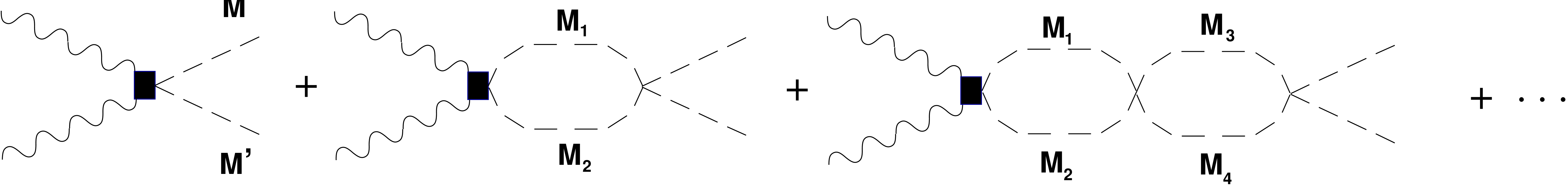
Figure 3: Diagrammatic series which gives rise to the FSI from a general $\gamma\gamma\rightarrow M\,M^{\prime}$ vertex.

The one loop contribution involving charged kaons can be obtained from eq. (5) by changing the amplitude $-(s-m_{\pi}^{2})/f^{2}$ by the corresponding $K^{+}K^{-}\rightarrow\pi^{0}\pi^{0}$ one and $m_{\pi}^{2}\rightarrow m_{K}^{2}$ in the rest of the formula. This is generalized to any meson-meson in the final state by changing the corresponding meson-meson amplitude.

Figure 4: One loop correction for the $\gamma\gamma\rightarrow M_{3}M_{4}$ tree level amplitude through the exchange of a resonance $R$ in the crossed channels. $M_{1}$ and $M_{2}$ are the intermediate states in the loop and $k$, $k^{\prime}$ are the momenta of the incoming photons.

We can also apply a similar procedure to account for FSI in the terms generated by vector and axial resonance exchange discussed in section 2. For this purpose we take the diagrams of fig. 4 and then the contribution of these one loop corrections, plus the extra iterations in the meson-meson amplitude discussed above, can be easily taken into account by means of

$$t_{R,M_{3}M_{4}}=\sum_{M_{1}M_{2}}\tilde{t}_{R,M_{1}M_{2}}t_{M_{1}M_{2},M_{3}M_{4}}$$

where

$$\tilde{t}_{R,M_{1}M_{2}}=i\int\frac{d^{4}q}{(2\pi)^{4}}t^{\prime}_{R},_{M_{1}M_{2}}\,\frac{1}{q^{2}-m_{1}^{2}+i\epsilon}\,\,\frac{1}{(P-q)^{2}-m_{2}^{2}+i\epsilon}$$ (7)

where once again the on shell strong meson-meson amplitude factorizes outside the integral.

The electromagnetic amplitude has a different structure to the strong one and must be kept inside the integral. In eq. (7) $P=(\sqrt{s},\vec{0})$ is the total fourmomentum of the $\gamma\gamma$ system and $m_{1},m_{2}$ the masses of the intermediate $M_{1},M_{2}$ mesons. In addition, and in analogy to the work of ref. [16], the integral over $|\vec{q}|$ in eq. (7) is cut at $q_{max}=0.9\,GeV$.

One can justify the accuracy of factorizing the strong amplitude for the loops with crossed exchange of resonances. Take for instance, eq.(2) for the exchange of the axial resonance and assume the limit $M_{A}\rightarrow\infty$ . From this equation we see that in this limit $t^{\prime}_{A}$ can be factorized outside the integral of eq. (7). Then if one takes the off shell part of the strong amplitude one cancells the propagators in eq. (7), after the $q^{0}$ integration, and obtains a result of the type $\Lambda^{2}t^{\prime}_{A}$ ($\Lambda$ is the cut off, $q_{max}$), which would renormalize the effective $t^{\prime}_{A}$ amplitude and since we are taking the physical value for the coupling constants this term should be omitted. These arguments are shown in detail in ref. [16]. A similar argumentation can be done for the exchange of vector mesons. Since we are dealing with real photons the intermediate axial or vector mesons are always off shell and the large mass limit is a sensible approximation. This implies that the error in the real part of the loops shown in fig. 4, in the way we estimate it, has an expansion in powers of $M_{R}^{-2}$ such that for $M_{R}\rightarrow\infty$ is zero. In this way if we call $\Delta_{\pi}$ the relative desviation between the exact value for the real part coming from eq. (5), $M_{R}=m_{\pi}$, and the value we would obtain following the procedure in eq. (7), then the relative error for a resonance mass $M_{R}$ would be $\Delta_{R}\simeq\Delta_{\pi}\bigl{[}\frac{m_{\pi}}{M_{R}}\bigr{]}^{2}$ which results in uncertainties below the level of 5$\%$ for $M_{R}$ about 800 $MeV$.

One of the limitations of the unitary method for meson-meson interaction of [16] is the lack of crossing symmetry. The unitarization is done in the s-channel but not in the t or u channels. In practice this limitation means that one should not use crossing symmetry to relate crossed channels. Instead, when the amplitude of these crossed channels has to be evaluated one redefines the new s-channel and applies then the method. The left hand cut neglected in our procedure is expected to be less important at high energies because the physical energy is far away from the cut. On the other hand, at low energies the loops and counterterms are in any case less important and are dominated by those of the s-channel unitarity considered here. These arguments are qualitative but they have been put in quantitative form in [34, 35] and the corrections are at the level of $2\%$, even at energies near the two pion threshold.

3.2 S-wave $T=2$ strong $\pi\pi$ amplitude

In the work of ref. [16] the $L=0$ and $T=0$, $T=1$ meson-meson amplitudes are evaluated. For the $\gamma\gamma\rightarrow\pi\pi$ we need also the $T=2$ channel. For this purpose we extend the work of ref. [16] to the $T=2$ channel. In this latter case we have only pions since $K\bar{K}$ or $\pi^{0}\eta$ does not couple to $T=2$. We get then

$$t^{(T=2)}=\frac{V^{(T=2)}}{1-GV^{(T=2)}}$$ (8)

where from ref. [16]

$$G(s)=\int_{0}^{q_{max}}dq\frac{q^{2}}{2\pi^{2}}\,\frac{1}{\omega(P^{02}-4\omega^{2}+i\epsilon)}$$ (9)

with $\omega=(\vec{q}\,^{2}+m^{2}_{\pi})^{1/2}$. The potential $V^{(T=2)}$ is given by

$$V^{(T=2)}=\frac{1}{2}\,\frac{s-2m_{\pi}^{2}}{f^{2}}$$ (10)

where following again the notation of ref. [16] we used the “unitary” normalization for the states

$$|\pi\pi,T=2,T_{3}=0>=-\frac{1}{\sqrt{12}}\,|\pi^{+}(\vec{q})\pi^{-}(-\vec{q})+\pi^{-}(\vec{q})\pi^{+}(-\vec{q})-2\pi^{0}(\vec{q})\pi^{0}(-\vec{q})>$$ (11)

This normalization (with an extra normalization $(1/\sqrt{2}$) is introduced in order to use the standard formula for the phase shifts when using identical particles

$$t^{(T=2)}=-\frac{8\pi\sqrt{s}}{2i}\,\frac{e^{2i\delta}-1}{p}$$ (12)

where $p$ is the CM momentum of the pion. The physical amplitude is given by $t(\theta)+t(\pi-\theta)$ and in S-wave this amounts to multiplying by a factor two the amplitude obtained in eq. (8).

In fig. 5 we show the phase shifts of $\pi\pi$ in $L=0$ and $T=2$ and compare them with the experimental results of ref. [36, 37, 38]. We see an agreement with the experimental results up to about $\sqrt{s}=0.8\,\,GeV$.

Figure 5: $\delta_{TL}=\delta_{20}$ phase shifts for the elastic $\pi\pi$ amplitude whith $L=0$ and $T=2$ from threshold to $0.8$ $GeV$. The squares are from [36], circles from [37] and the triangles from [38].

In order to have some more accurate results at energies higher than $\sqrt{s}=0.8\,\,GeV$ we take the experimental phase shifts. This has irrelevant consequences in the $\gamma\gamma\rightarrow\pi^{+}\pi^{-}$ amplitude and introduces changes of the order of 10$\%$ at high energies in the $\gamma\gamma\rightarrow\pi^{0}\pi^{0}$ channel with respect to using the $T=2$ amplitude of our theoretical approach.

3.3 D-wave contribution

As one can see from ref. [28] (see fig. 7 of this reference) the Born term in $\gamma\gamma\rightarrow\pi^{+}\pi^{-}$ is given essentially by the $(0,0)$ and $(2,2)$ partial waves, in $(J,\lambda)$ notation, where $J$ is the angular momentum and $\lambda$ is the difference of helicities of the two photons.

The $(0,0)$ component has already been taken care of in section 3.1. For the $(2,2)$ component we take the results of ref. [28], obtained using dispersion relations, and which are parametrized in the form

$$t_{BC}^{(2,2)}=\biggl{[}\frac{2}{3}\,\chi_{22}^{T=0}\,e^{i\delta_{20}}+\frac{1}{3}\,\chi_{22}^{T=2}\,e^{i\delta_{22}}\biggr{]}\,t_{B}^{(2,2)}$$ (13)

where $t_{B}^{(2,2)}$ is the $(2,2)$ component of the Born term, $\delta_{20}$ and $\delta_{22}$ are the phase shifts of $\pi\pi\rightarrow\pi\pi$ in $L=2$, $T=0$ and $T=2$ respectively. $\chi_{22}^{T=0}$ is a function which is approximately given by

$$\chi_{22}=1-(\frac{s}{s_{0}})^{2}$$ (14)

We see from fig. 8 of ref. [28] that $s_{0}\simeq 1.20-1.25\,\,GeV$. We take $s_{0}=1.3\,\,GeV$ in our calculations which leads to slightly better results. Finally we make use that $\chi_{22}^{T=2}\simeq 1$ as stated in ref. [28].

For the phase shifts $\delta_{20}$ we make use of the fact that this channel is dominated by the $f_{2}(1270)$ resonance (see section 4 for amplitudes of resonant terms). In fig. 6 we show the phase shifts of this channel calculated from the resonant amplitude compared with experiment and the agreement with the data is good.

Figure 6: $\delta_{TL}=\delta_{02}$ phase shifts for the elastic $\pi\pi$ amplitude with $L=2$ and $T=0$ from threshold to $1.4$ $GeV$. This curve is given only through the exchange of the $f_{2}(1270)$ resonance. The experimental data are from ref. [36], squared points and [39] for the empty circles.

For the $\gamma\gamma\rightarrow K^{+}K^{-}$ reaction the Born term contribution in $L=2$ is small compared to the one in S-wave up to about $\sqrt{s}=1.4\,\,GeV$, due to the large $K$ mass. Moreover, this contribution is further reduced with a similar formula as eq. (13) with $s_{0}$ around the mass of the lowest resonance in each partial wave ($s_{0}\simeq 1.3$ $GeV$ corresponding to the mass of the $f_{2}$ ($T=0$) and $a_{2}$ ($T=1$) resonances) [28, 30]. This allows us to neglect this term to a good approximation in the range $\sqrt{s}<1.4$ $GeV$ where we are interested.

Given the fact that the result of eq. (13) is generated by dispersion relations using empirical input, the amplitude of eq. (13) should also take into account the $L=2$ contribution which is generated by our vector and axial resonance exchange in the crossed channels. Hence we consider explicitly only the S-wave part of the resonance exchange as discussed in section 3.1.

Apart from this background terms in $L=2$, we have the contribution of the $L=2$ resonances which we discuss below.

4 Direct coupling to the $f_{2}(1270)$ and $a_{2}(1320)$ resonances.

Here we follow a standard procedure to include the resonances in the same way as done in ref. [7].

As it is usually done [7, 11] we consider only the $\lambda=2$ contribution and hence we have the parametrization

$$t^{(2,2)}_{R}=i16\pi\sqrt{\frac{20\pi}{\beta(s)}}BW(s)(\Gamma_{\gamma\gamma}^{(2)})^{1/2}\,Y_{22}(\cos\theta,\varphi)$$ (15)

where $\Gamma_{\gamma\gamma}^{(22)}$ is the resonance decay width into two photons with opposite helicity. Furthermore

$$BW(s)=\frac{m_{R}\sqrt{\Gamma(\sqrt{s})Br(M\bar{M})}}{s-m_{R}^{2}+im_{R}\Gamma(\sqrt{s})}$$ (16)

$$\Gamma(\sqrt{s})=\Gamma(m_{R})\,\Biggl{[}\frac{p(\sqrt{s})}{p(m_{R})}\Biggr{]}^{5}\,\frac{m_{R}}{\sqrt{s}}\,\frac{h(\sqrt{s})}{h(m_{R})}$$ (17)

$$h(\sqrt{s})\,\propto[9+3(pr)^{2}+(pr)^{4}]^{-1}$$ (18)

where $h(\sqrt{s})$ is a decay form factor [40], $r$ is the effective interaction radius taken as $r\simeq 1\,fm$, $p$ is the CM momentum of the $M\bar{M}$ system and $\Gamma(\sqrt{s})$ the total width of the resonance, $Br(M\bar{M})$ is the branching ratio for the decay into the $M\bar{M}$ system such that $\Gamma(\sqrt{s})\,Br(M\bar{M})S_{i}$ is the partial decay width into the $M\bar{M}$ channel, with $S_{i}=1/2,1$ depending on whether the final $M\bar{M}$ state contains or does not contain two identical particles. Given the fact that there is an important interference for the $\gamma\gamma\rightarrow\pi^{+}\pi^{-}$ reaction between the Born term in the $(2,2)$ channel and the contribution of the resonance $f_{2}(1270)$, it is then important that the total (2,2) amplitude is properly unitarized and this is accomplished with the modification of the Born piece used in eq. (13). On the other hand, the choice of a constant value $r=1$ fm reproduces well the resonance around the peak but overestimates the tail of the resonance. We have chosen $r$ energy dependent in order to reproduce the T=0, L=2 phase shifts in terms of the $f_{2}(1270)$ resonance. We take $r=(\sqrt{s}-2\;m_{\pi})/9\;m_{\pi}$ which as can be seen in Fig. 6 reproduces very well the phase shifts $\delta_{02}$.

We take the following parameters for the resonances by means of which the resonance strength, position and widths are well reproduced:

$a)f_{2}(1270)$

$$\begin{array}[]{llll}m_{R}=1275\,MeV&\Gamma_{R}=185\,MeV&Br(\pi\pi)\Gamma_{\gamma\gamma}^{(2)}=2.64\,KeV&Br(K\bar{K})\Gamma_{\gamma\gamma}^{(2)}=0.1\,KeV\end{array}$$ (19)

$b)a_{2}(1320)$

$$\begin{array}[]{llll}m_{R}=1318\,MeV&\Gamma_{R}=105\,MeV&Br(\eta\pi)\Gamma_{\gamma\gamma}^{(2)}=0.19\,KeV&Br(K\bar{K})\Gamma_{\gamma\gamma}^{(2)}=0.1\,KeV\end{array}$$ (20)

These values are compatible with those of the Particle Data Group [41].

5 Final amplitudes for the $\gamma\gamma\rightarrow M\bar{M}$ reaction

Let us introduce some notation in order to proceed to sum the different amplitudes. We denote by $\tilde{t}_{\chi\pi}(\tilde{t}_{\chi K})$ the chiral amplitude to order $O(p^{4})$ with charged $\pi(K)$ intermediate states from eq. (5) eliminating the strong amplitude to order $O(p^{2})$ which factorizes the amplitude

$$\tilde{t}_{\chi\pi}=\,-\frac{\epsilon_{1}\epsilon_{2}}{16\pi^{2}}\,2e^{2}\;\left\{1+\frac{m_{\pi}^{2}}{s}\,[ln\left(\frac{1+(1-4m_{\pi}^{2}/s)^{\frac{1}{2}}}{1-(1-4m_{\pi}^{2}/s)^{\frac{1}{2}}}\right)-i\pi]^{2}\right\}$$ (21)

with the obvious change $m_{\pi}^{2}\rightarrow m_{K}^{2}$ for $\tilde{t}_{\chi K}$ and its analytical extrapolation below threshold.

We denote by $t_{R}(R\equiv\rho,\omega,A)$ the tree level resonance on shell contributions in S-wave, which are given in refs. [20, 21]. In our normalization these will be

$$\begin{array}[]{l}t_{\rho}=2e^{2}\epsilon_{1}\epsilon_{2}R_{\rho}[\frac{\displaystyle{m_{\rho}^{2}}}{\displaystyle{\beta(s)}}ln\left(\frac{\displaystyle{1+\beta(s)+\frac{s_{\rho}}{s}}}{\displaystyle{1-\beta(s)+\frac{s_{\rho}}{s}}}\right)-s]\\[17.22217pt] t_{\omega}=2e^{2}\epsilon_{1}\epsilon_{2}R_{\omega}[\frac{\displaystyle{m_{\omega}^{2}}}{\displaystyle{\beta(s)}}ln\left(\frac{\displaystyle{1+\beta(s)+\frac{s_{\omega}}{s}}}{\displaystyle{1-\beta(s)+\frac{s_{\omega}}{s}}}\right)-s]\\[17.22217pt] t_{A}=-2e^{2}\epsilon_{1}\epsilon_{2}\frac{\displaystyle{(L^{r}_{9}+L^{r}_{10})}}{\displaystyle{f^{2}}}[\frac{\displaystyle{s_{A}}}{\displaystyle{2\beta(s)}}ln\left(\frac{\displaystyle{1+\beta(s)+\frac{s_{A}}{s}}}{\displaystyle{1-\beta(s)+\frac{s_{A}}{s}}}\right)+s]\end{array}$$ (22)

where $s_{\omega}=2(m_{\omega}^{2}-m_{\pi}^{2}),s_{\rho}=2(m_{\rho}^{2}-m_{\pi}^{2}),s_{A}=2(m_{A}^{2}-m_{\pi}^{2})$ for $\gamma\gamma\rightarrow\pi^{+}\pi^{-}$ and $s_{A}=2(m_{A}^{2}-m_{K}^{2})$ for $\gamma\gamma\rightarrow K^{+}K^{-}$.

Since we have direct coupling to the resonances $f_{2}$ and $a_{2}$ with helicity 2, it is convenient to work in the helicity basis for the amplitudes. By taking

$$\begin{array}[]{ll}\epsilon_{+}=-\frac{1}{\sqrt{2}}(\epsilon_{x}+i\epsilon_{y})&\epsilon_{-}=\frac{1}{\sqrt{2}}(\epsilon_{x}-i\epsilon_{y})\end{array}$$ (23)

The Born amplitude of eq. (1) is then separated into

$$\begin{array}[]{l}t^{(0)}=t^{\lambda=0}_{B}=t^{++}_{B}=i\frac{2e^{2}(1-\beta^{2})}{1-\beta^{2}cos^{2}\theta}\\[8.61108pt] t^{(2)}=t^{\lambda=2}_{B}=t_{B}^{+-}=-i\frac{2e^{2}\beta^{2}e^{2i\phi}\sin^{2}\theta}{1-\beta^{2}cos^{2}\theta}\end{array}$$ (24)

where $\beta\equiv\beta(s)=(1-4m^{2}/s)^{1/2}$ with $m$ the mass of the corresponding charged meson.

The amplitudes which we have introduced $t_{R},\tilde{t}_{\chi\pi},\tilde{t}_{\chi K},\tilde{t}_{R,M_{1}M_{2}}$ only contribute in S-wave and hence only have helicity zero. Thus, by means of eq. (23) we have $t^{++}=it$ where $t$ stands here for the different amplitudes.

Note that in $t^{++}$ one has contributions from $(J,\lambda)=(0,0),(2,0)$… . However, we also mentioned that the $(2,0)$ component of the Born term is negligible. On the other hand following ref. [28] this Born component, plus corrections from crossed channels, is given by an equation like eq. (13) and then the relative smallness remains. Hence we neglect this kind of contributions and similarly for the $t^{+-}$ amplitude for partial waves higher than 2.

For simplicity we take the full $t^{+-}_{B}$ amplitude in eq. (13) rather than $t_{B}^{(2,2)}$ since the higher multipoles (4,2), (6,2), … contributions are also very small. We will call $t_{BC}^{(2)}$ this amplitude. The amplitudes used below are the physical amplitudes with proper normalization of the states, not the “unitary” normalization amplitudes of eq. (8), (10) or those of ref. [16] for symmetrical pionic states. Note also that $t_{A},t_{B},t_{f}^{(2,2)},t_{a}^{(2,2)}$ depend on the channel as stated in eqs. (22), (24), (15-18).

After this discussion we can already write the amplitudes:

$1)\;\gamma\gamma\rightarrow\pi^{+}\pi^{-}$

$$\begin{array}[]{l}t^{(0)}=t^{(0)}_{B}+i\{t_{A}+t_{\rho}+(\tilde{t}_{A\pi^{+}\pi^{-}}+\tilde{t}_{\rho\pi^{+}\pi^{-}}+\tilde{t}_{\chi\pi})t_{\pi^{+}\pi^{-},\pi^{+}\pi^{-}}\,+\\ +\,(\tilde{t}_{AK^{+}K^{-}}+\tilde{t}_{\chi K})t_{K^{+}K^{-},\pi^{+}\pi^{-}}+(\tilde{t}_{\rho\pi^{0}\pi^{0}}+\tilde{t}_{\omega\pi^{0}\pi^{0}})t_{\pi^{0}\pi^{0},\pi^{+}\pi^{-}}\}\\ t^{(2)}=t^{(2)}_{BC}+t_{f_{2}}^{(22)}\end{array}$$ (25)

where

$$\begin{array}[]{l}t_{\pi^{+}\pi^{-},\pi^{+}\pi^{-}}=\frac{1}{3}t^{I=0}+\frac{1}{6}t^{I=2}\\ t_{\pi^{0}\pi^{0},\pi^{+}\pi^{-}}=\frac{1}{3}t^{I=0}-\frac{1}{3}t^{I=2}\\ t_{K^{+}K^{-},\pi^{+}\pi^{-}}=\frac{1}{\sqrt{6}}t^{I=0}\end{array}$$ (26)

$2)\gamma\gamma\rightarrow\pi^{0}\pi^{0}$

$$\hskip 56.9055pt\begin{array}[]{l}-it^{(0)}=t_{\omega}+t_{\rho}+(\tilde{t}_{\rho\pi^{0}\pi^{0}}+\tilde{t}_{\omega\pi^{0}\pi^{0}})t_{\pi^{0}\pi^{0},\pi^{0}\pi^{0}}+\\ +(\tilde{t}_{A\pi^{+}\pi^{-}}+\tilde{t}_{\rho\pi^{+}\pi^{-}}+\tilde{t}_{\chi\pi})t_{\pi^{+}\pi^{-},\pi^{0}\pi^{0}}+(\tilde{t}_{\chi K}+\tilde{t}_{AK^{+}K^{-}})t_{K^{+}K^{-},\pi^{0}\pi^{0}}\\ t^{(2)}=t_{f_{2}}^{(2,2)}\end{array}$$ (27)

$$\begin{array}[]{l}t_{\pi^{0}\pi^{0},\pi^{0}\pi^{0}}=\frac{1}{3}t^{I=0}+\frac{2}{3}t^{I=2}\\ t_{K^{+}K^{-},\pi^{0}\pi^{0}}=\frac{1}{\sqrt{6}}t^{I=0}\\ t_{\pi^{+}\pi^{-},\pi^{0}\pi^{0}}=t_{\pi^{0}\pi^{0},\pi^{+}\pi^{-}}\end{array}$$ (28)

3) $\gamma\gamma\rightarrow\pi^{0}\eta$

$$\begin{array}[]{l}-it^{(0)}=(\tilde{t}_{AK^{+}K^{-}}+\tilde{t}_{\chi K})t_{K^{+}K^{-},\pi^{0}\eta}\\ t^{(2)}=t^{(2,2)}_{a_{2}}\end{array}$$ (29)

$$t_{K^{+}K^{-},\pi^{0}\eta}=-\frac{1}{\sqrt{2}}t^{I=1}$$ (30)

4) $\gamma\gamma\rightarrow K^{+}K^{-}$

$$\begin{array}[]{l}t^{(0)}=t_{B}^{(0)}+i\{t_{A}+(\tilde{t}_{A\pi^{+}\pi^{-}}+\tilde{t}_{\rho\pi^{+}\pi^{-}}+\tilde{t}_{\chi\pi})t_{\pi^{+}\pi^{-},K^{+}K^{-}}+\\ +(\tilde{t}_{\rho\pi^{0}\pi^{0}}+\tilde{t}_{\omega\pi^{0}\pi^{0}})t_{\pi^{0}\pi^{0},K^{+}K^{-}}+(\tilde{t}_{AK^{+}K^{-}}+\tilde{t}_{\chi K})t_{K^{+}K^{-},K^{+}K^{-}}\}\\ t^{(2)}=t^{(2,2)}_{f_{2}}+t^{(2,2)}_{a_{2}}\end{array}$$ (31)

$$\begin{array}[]{l}t_{\pi^{+}\pi^{-},K^{+}K^{-}}=t_{K^{+}K^{-},\pi^{+}\pi^{-}}\\ t_{\pi^{0}\pi^{0},K^{+}K^{-}}=t_{K^{+}K^{-},\pi^{0}\pi^{0}}\\ t_{K^{+}K^{-},K^{+}K^{-}}=\frac{1}{2}t^{I=0}+\frac{1}{2}t^{I=1}\end{array}$$ (32)

$5)\gamma\gamma\rightarrow K^{0}\bar{K}^{0}$

$$\begin{array}[]{l}-it^{(0)}=(\tilde{t}_{A\pi^{+}\pi^{-}}+\tilde{t}_{\rho\pi^{+}\pi^{-}}+\tilde{t}_{\chi K})t_{\pi^{+}\pi^{-},K^{0}\bar{K}^{0}}+\\ +(\tilde{t}_{\rho\pi^{0}\pi^{0}}+\tilde{t}_{\omega\pi^{0}\pi^{0}})t_{\pi^{0}\pi^{0},K^{0}\bar{K}^{0}}+(\tilde{t}_{AK^{+}K^{-}}+\tilde{t}_{\chi K})t_{K^{+}K^{-},K^{0}\bar{K}^{0}}\\ t^{(2)}=t^{(2,2)}_{f_{2}}-t^{(2,2)}_{a_{2}}\end{array}$$ (33)

$$\begin{array}[]{l}t_{\pi^{+}\pi^{-},K^{0}\bar{K}^{0}}=t_{K^{+}K^{-},\pi^{+}\pi^{-}}\\ t_{\pi^{0}\pi^{0},K^{0}\bar{K}^{0}}=t_{K^{+}K^{-},\pi^{0}\pi^{0}}\\ t_{K^{+}K^{-},K^{0}\bar{K}^{0}}=\frac{1}{2}t^{I=0}-\frac{1}{2}t^{I=1}\end{array}$$ (34)

It is interesting to note that the isoscalar $f_{2}$ and isovector $a_{2}$ resonances interfere constructively in $\gamma\gamma\rightarrow K^{+}K^{-}$ and destructively in $\gamma\gamma\rightarrow K^{0}\bar{K}^{0}$ as shown at the end of eqs. (31) and (33). This fact has been predicted [42] long before its observation (see experimental results in figs. 11 and 12).

The width for $\omega\rightarrow\gamma\eta$ is about two orders of magnitude smaller than for $\omega\rightarrow\gamma\pi^{0}$, resulting in a smaller coupling. For this reason we omit the contributions involving the $\omega\rightarrow\gamma\eta$ coupling which should appear in $\gamma\gamma\rightarrow\pi^{0}\eta$, $K\bar{K}$. We have, however, estimated the relevance of this term calculating the tree level and the final state interaction correction (only the imaginary part of this latter term) for the $\gamma\gamma\rightarrow\pi^{0}\eta$ channel, where it is more relevant. We have seen that it gives small corrections which will be shown in section $6$.

6 Differential and integrated cross sections for $\gamma\gamma\rightarrow M\bar{M}$

In terms of the $t^{(0)}$ and $t^{(2)}$ amplitudes we have

$$\frac{d\sigma}{d\cos\theta}=\frac{\beta}{64\pi s}[|t^{(0)}|^{2}+|t^{(2)}|^{2}]$$ (35)

and the cross section integrated for $|\cos\theta|<Z$, as given in some experiments,

$$\sigma=2\int_{0}^{Z}\frac{d\sigma}{d\cos\theta}\,d\cos\theta$$ (36)

Figure 7: The integrated cross section for $\gamma\gamma\rightarrow\pi^{0}\pi^{0}$ with $Z=0.8$ compared with the data from ref. [1] and ref. [2], the latter normalized in the $f_{2}(1270)$ peak region.

In fig. 7 we show the cross section for $\gamma\gamma\rightarrow\pi^{0}\pi^{0}$ integrated up to $Z=0.8$ compared to the data of Crystal Ball [1] and JADE [2]. The data of Crystal Ball are normalized while those of JADE correspond to an unnormalized distribution. We have chosen a normalization of this latter data such that in the large peak of the cross section corresponding to the $f_{2}(1270)$ resonance the two cross sections have the same strength. Our results are in agreement with those of the Crystall Ball experiment at very low energies, where they agree with those of the two loop calculations in $\chi PT$ [24], and for $\sqrt{s}>0.6$ $GeV$. For $0.4<\sqrt{s}<0.6$ our results lie between those of the Crystall Ball and JADE experiments. The calculation shows a broad bump in this region, a consequence of the presence of the $\sigma$ meson pole in the L=0, T=0 channel around $(470+i200)$ $MeV$. The data around the $f_{2}$ resonance is well reproduced.

It is quite interesting to see that the $f_{0}$ resonance shows up as a small peak in the cross section, in the lines of what is observed in both experiments. The smallness of the peak in our calculation is due to interference with the $\omega$ contribution.

Figure 8: The integrated cross sections for $\gamma\gamma\rightarrow\pi^{+}\pi^{-}$ with Z=0.6 compared with the experimental data from refs. [5, 4, 3] respectively from up to down in the figure as indicated in the text. We also show the Born term calculation.

In fig. 8 we show the cross section for $\gamma\gamma\rightarrow\pi^{+}\pi^{-}$ integrated up to $Z=0.6$ compared to the experimental data of the SLAC-PEP-TPC/ TWO GAMMA [3], SLAC-PEP-MARK II [4] and DESY-PETRA-CELLO [5] collaborations. The agreement with the data is good in general particularly with the results of MARK-II. We can see that the $f_{0}$ resonance does not show up significantly in the data nor in the calculation. Note also that we reproduce the peak corresponding to the $f_{2}(1270)$ both in figs. 7 and 8.

Figure 9: Differential cross sections for $\gamma\gamma\rightarrow\pi^{+}\pi^{-}$ in three energy regions compared with the data of MARKII [4] and CELLO[5] around the $f_{2}(1270)$ resonance peak.

In figs. 9a,b,c we present differential cross sections for $\gamma\gamma\rightarrow\pi^{+}\pi^{-}$ in three different energy regions around the peak of the $f_{2}(1270)$ resonance. In general one observes a good agreement with the data. Note also that these differential cross sections were used in ref. [29] together with the former cross section in order to justify the existence of the resonance $f_{0}(1100)$. We see that we reproduce the data without the need to introduce this resonance. The use of our precise L = 0 amplitudes and the unitary scheme followed here produce the necessary S-wave contribution to weaken the angular dependence of the cross sections as observed by experiment.

Figure 10: Integrated cross section for $\gamma\gamma\rightarrow\pi^{0}\eta$ with $Z=0.9$ $GeV$ compared with the experimental data from ref. [2] and ref. [6], the latter normalized in the $a_{2}(1320)$ peak region. We show our calculations for the S-wave contribution. The results with and without the $\omega$ contribution are also shown.

In fig. 10 we show our results for the $\gamma\gamma\rightarrow\pi^{0}\eta$ compared to the data of DESY-PETRA-JADE [2] and DESY-DORIS-CRYSTALL-BALL [6] ($Z=0.9$). The data of ref. [6] are normalized but those of ref. [2] have arbitrary normalization. In the figure we have normalized them such that they have the same strength as those of ref. [6] in the $a_{2}(1320)$ peak. We can see a fair agreement of our results with the data, both around the $a_{2}(1320)$ resonance (the parameters of which are taken from the particle data tables) and for the peak around the $a_{0}(980)$ resonance, which results naturally from the use of our unitarized meson-meson amplitudes. We also show in the figure the S-wave contribution alone, which includes the $a_{0}(980)$ peak. We reproduce the data in the intermediate energy between the two resonances without the need to introduce an additional background, which has been sometimes assumed to come from a broad $a_{0}(1100-1300)$ resonance [11]. In the figure we also show the result including the contribution of the exchange of the $\omega$, estimated as indicated in section 2. We see negligible corrections in the peak of the $a_{0}$ and more significative changes around the minimum of the cross section.

In [43] the peak of the $a_{0}$ and the deep region were also reproduced without the inclusion of a background. However, as noted in ref. [11] the $\gamma\gamma\rightarrow K^{+}K^{-}$ amplitude was overestimated since the Born amplitude was used which is drastically reduced due to final state interaction, as we shall see below. On the other hand the exchange of an axial resonance, as we do here, was not included in ref. [43] and this is essential to reproduce the strength of the $a_{0}(980)$ peak. Indeed if we take $L_{9}^{r}+L_{10}^{r}=0$ we get a strength of the peak around one third of the experimental strength.

Figure 11: Integrated $\gamma\gamma\rightarrow K^{+}K^{-}$ from threshold to 1.45 $GeV$ compared with the experimental data from ref. [7]. We also show the Born contribution and the S-wave background.

In fig. 11 we show results for $\gamma\gamma\rightarrow K^{+}K^{-}$ together with the data of DESY-DORIS-ARGUS [7]. We also show there the contribution of the Born term without corrections and the background in S-wave. The cross section is also well reproduced in this channel. The most striking feature in this figure is the drastic reduction of the Born term contribution due to FSI and to the crossed channel contributions. Around $\sqrt{s}=1070\;\,MeV$ this reduction is more than a factor ten. The need to reduce drastically the Born contribution had been pointed out before but no theoretical justification had been found so far [11].

Figure 12: Integrated $\gamma\gamma\rightarrow K^{0}\bar{K}^{0}$ from threshold to 1.45 $GeV$ compared with the data from ref. [8, 9] respectively as it is indicated in the figure from up to down. We also show the S-wave contribution.

In fig. 12 we show the results for $\gamma\gamma\rightarrow K^{0}\bar{K}^{0}$ compared to the data of DESY-PETRA-TASSO [8] and DESY-PETRA-CELLO [9]. The results are compatible with the data, which, however, have large errors. We also show the background of S-wave without the contribution of the $f_{2}$ and $a_{2}$ resonances. The background found is small as expected, but not because of the lack of a Born term, but because of cancellations between important contributions which were also responsible for the reduction of the $\gamma\gamma\rightarrow K^{+}K^{-}$ Born term.

7 Partial decay width to two photons of the $f_{0}(980)$ and $a_{0}(980)$.

In ref. [16] the partial decay widths of the $f_{0}(980)$ and $a_{0}(980)$ resonances into $\pi\pi,K\bar{K}$ or $\pi^{0}\eta$ were evaluated. In this section we complete the information evaluating the partial decay widths into $\gamma\gamma$.

From our amplitudes in eqs. (30) in isospin $T=1$ and eq. (32) for the isospin $T=0$ part, by taking the terms which involve the strong $M\bar{M}\rightarrow M\bar{M}$ amplitude, we isolate the part of the $\gamma\gamma\rightarrow M\bar{M}$ which proceeds via the resonances $a_{0}$ and $f_{0}$ respectively. In the vicinity of the resonance the amplitude proceeds as $M\bar{M}\rightarrow R\rightarrow M\bar{M}$. Then we eliminate the $R\rightarrow M\bar{M}$ part of the amplitude plus the $R$ propagator and remove the proper isospin Clebsch Gordan coefficients for the final states (1 for $\pi^{0}\eta$ and $-1/\sqrt{2}$ for $K^{+}K^{-}$) and then we get the coupling of the resonances to the $\gamma\gamma$ channel. It is convenient to do this for the $K^{+}K^{-}$ final states because in the case of the pions one has a large background of the $\sigma$ resonance in the elastic amplitude.

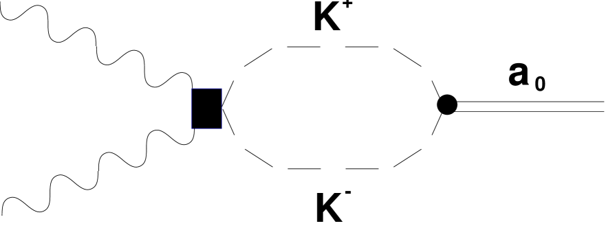
Figure 13: $g_{a\gamma\gamma}$ through $K^{+}K^{-}$ intermediate states, connecting the $a_{0}$ resonance with the two photons.

Diagrammatically this is represented in fig. 13 for the $a_{0}$ case. The $g_{a_{0}\gamma\gamma}$ coupling is then given by

$$g_{a_{0}\gamma\gamma}=-\frac{g_{a_{0}K\bar{K}}}{\sqrt{2}}\,[\tilde{t}_{\chi K}+\tilde{t}_{AK^{+}K^{-}}]$$ (37)

where $g_{a_{0}\gamma\gamma}$ is the coupling of the $a_{0}$ to the $K\bar{K}$ system evaluated in ref. [16]. The $-1/\sqrt{2}$ in front of eq. (38) is the Clebsch Gordan coefficient of $|K\bar{K},T=1>$ to $K^{+}K^{-}$. Following ref. [16] the decay width of $a_{0}\rightarrow\gamma\gamma$ is given by

$$\Gamma_{a_{0}}^{\gamma\gamma}=\frac{1}{16\pi^{2}}\,\frac{1}{2}\,\sum_{\lambda_{1},\lambda_{2}}\,\int^{\infty}_{0}\,dW\,\frac{q}{W^{2}}\,|g_{a_{0}\gamma\gamma}|^{2}\,\frac{\Gamma_{a_{0}}(W)}{(M_{a_{0}}-W)^{2}+(\frac{\Gamma_{a_{0}}(W)}{2})^{2}}$$ (38)

where $\lambda_{1},\lambda_{2}$ are the photon polarizations and $W=\sqrt{s}$. The coupling $g_{a_{0}K\bar{K}}$ is evaluated in ref. [16] in terms of $Im\,t_{11}$ of $K\bar{K}\rightarrow K\bar{K},T=1$ amplitude and hence we find

$$\Gamma_{a_{0}}^{\gamma\gamma}=\frac{-1}{16\pi^{2}}\,\int^{\infty}_{0}\,dW\,\frac{q}{W^{2}}\,4M_{R}\,|\frac{\tilde{t}_{\chi K}+\tilde{t}_{AK^{+}K^{-}}}{\sqrt{2}}|^{2}\,Im\,t_{11}$$ (39)

where the lower limit in practice is the threshold for the lightest $M\bar{M}$ pair in this channel where $Imt_{11}\neq 0$ ($\pi^{0}\eta$ in this case). The integral extends over $W$ about $2\,\Gamma$ above and below $M_{R}$, the pole mass $M_{a_{0}}=1009\;\,MeV$, with $\Gamma=112$ $MeV$. We thus obtain

$$\Gamma_{a_{0}}^{\gamma\gamma}=0.78\;KeV$$ (40)

and the related quantity

$$\Gamma_{a_{0}}^{\gamma\gamma}\frac{\Gamma_{a_{0}}^{\eta\pi}}{\Gamma_{a_{0}}^{tot}}=0.49\;\,KeV$$ (41)

For the $f_{0}$, apart from $K^{+}K^{-}$ intermediate states we have $\pi^{+}\pi^{-}$, and also $\pi^{0}\pi^{0}$ through the $\omega$ exchange. Thus we have

$$g_{f_{0}\gamma\gamma}=-\frac{g_{f_{0}K\bar{K}}}{\sqrt{2}}(\tilde{t}_{AK^{+}K^{-}}+\tilde{t}_{\chi K})-\frac{g_{f_{0}\pi\pi}}{\sqrt{3}}(\tilde{t}_{A\pi^{+}\pi^{-}}+\tilde{t}_{\rho\pi^{+}\pi^{-}}+\tilde{t}_{\chi\pi}+\tilde{t}_{\rho\pi^{0}\pi^{0}}+\tilde{t}_{\omega\pi^{0}\pi^{0}})$$ (42)

Hence by writing the strong $g_{f_{0}K\bar{K}}$ and $g_{f_{0}\pi\pi}$ couplings in terms of the strong amplitudes we find

$$\begin{array}[]{l}\Gamma_{f_{0}}^{\gamma\gamma}=-\frac{1}{16\pi^{2}}\,\int^{\infty}_{0}\,dW\,\frac{q}{W^{2}}\,4M_{R}\,\left\{\right.|\frac{\chi_{K}}{\sqrt{2}}|^{2}Imt_{11}\\[8.61108pt] +|\frac{\chi_{\pi}}{\sqrt{3}}|^{2}\,\frac{(Re(t_{21}))^{2}}{Imt_{11}}\,-\sqrt{\frac{2}{3}}\,Re(t_{21})\hbox{Im(}\chi_{K}\chi_{\pi}^{*})\left.\right\}\end{array}$$ (43)

where for simplicity we have introduced the notation

$$\begin{array}[]{l}\chi_{K}=\tilde{t}_{\chi K}+\tilde{t}_{AK^{+}K^{-}}\\[8.61108pt] \chi_{\pi}=\tilde{t}_{A\pi^{+}\pi^{-}}+\tilde{t}_{\rho\pi^{+}\pi^{-}}+\tilde{t}_{\chi\pi}+\tilde{t}_{\omega\pi^{0}\pi^{0}}+\tilde{t}_{\rho\pi^{0}\pi^{0}}\end{array}$$ (44)

In this case we also integrate in $W$ $2\,\Gamma$ up and down $M_{f_{0}}(M_{f_{0}}=992\;\,MeV)$, with $\Gamma_{f_{0}}=25\,\,MeV$ [16].

Thus we get

$$\Gamma^{\gamma\gamma}_{f_{0}}=0.20\;\,KeV$$ (45)

The result of eq. (41) is larger than the results quoted in the particle data group [41], ($0.28\pm 0.04\pm 0.1$) KeV from ref. [2] and ($0.19\pm 0.07\pm 0.10$) KeV form ref. [6]. However, one should note that in the experimental analysis a background term is assumed while in our approach the strength around the $a_{0}$ peak in the $\gamma\gamma\rightarrow\pi^{0}\eta$ cross section comes from the $a_{0}$ excitation.

The result of eq. (45) is smaller than the average in the PDG [41] ($0.56\pm 0.11$) $KeV$, although consistent with some analyses, $(0.29\pm 0.07\pm 0.12)$ $KeV$ [4] and $(0.31\pm 0.14\pm 0.09)$ $KeV$ [1].

Eq. (43) has made use of a peculiar property of the $f_{0}$ resonance which is that the $t_{21}$ amplitude around the $f_{0}$ resonance can be approximately described by an ordinary Breit-Wigner form multiplied by the phase factor $e^{i\pi/2}$. This can be seen from the experimental phase shifts for $K\bar{K}\rightarrow\pi\pi$, T=0, L=0, which lie around $220$ degrees, ( see Fig. 4 of [16]). This fact was overlooked in the partial decay analysis of the $f_{0}$ resonance in [16]. This deficiency, together with some small numerical corrections which lead to a slightly smaller cut off of $\Lambda=1$ $GeV$, have been taken into account in a reanalysis of these partial decay widths in [44]. We use here this updated information.

8 Conclusions

We have presented here a unified theoretical approach for the reaction $\gamma\gamma\rightarrow M\bar{M}$ with $M\bar{M}=\pi^{+}\pi^{-},\pi^{0}\pi^{0},K^{0}\bar{K}^{0},\pi^{0}\eta$. An important new ingredient with respect to other works is the treatment of the S-wave $M\bar{M}$ amplitudes in $T=0$, $1$, which we have taken from a recent successful work based upon chiral symmetry. This allows us to treat accurately the strong final state interaction which plays a major role in this reaction.

We have also taken into account well established facts concerning the role of the exchange of vector and axial resonances in the $t$ and $u$ channels.

The direct coupling to the $f_{2}(1270)$ and $a_{2}(1320)$ resonances has been introduced explicitly in a standard way assuming dominance of the helicity two amplitudes, as customarily done.

With all these ingredients we study for the first time all these final mesonic states with a unified approach and obtain a general agreement in all channels up to about $\sqrt{s}=1.4\,MeV$.

Some results of our study are worth stressing:

1) The resonance $f_{0}(980)$ shows up weakly in $\gamma\gamma\rightarrow\pi^{0}\pi^{0}$ and barely in $\gamma\gamma\rightarrow\pi^{+}\pi^{-}$.

2) In order to explain the angular distributions of the $\gamma\gamma\rightarrow\pi^{+}\pi^{-}$ reaction we did not need the hypothetical $f_{0}(1100)$ broad resonance suggested in other works [29]. This also solves the puzzle of why it did not show up in the $\gamma\gamma\rightarrow\pi^{0}\pi^{0}$ channel. Furthermore, such resonance does not appear in the theoretical work of ref. [16], while the $f_{0}(980)$ showed up clearly as a pole of the $t$ matrix in $T=0$.

3) The resonance $a_{0}$ shows up clearly in the $\gamma\gamma\rightarrow\pi^{0}\eta$ channel and we reproduce the experimental results without the need of an extra background from a hypothetical $a_{0}(1100-1300)$ resonance suggested in ref. [11].

4) We have found an explanation to the needed reduction of the Born term in the $\gamma\gamma\rightarrow K^{+}K^{-}$ reaction in terms of final state interaction of the $K^{+}K^{-}$ system.

5) In the case of $\gamma\gamma\rightarrow K^{0}\bar{K}^{0}$ we find a small cross section, which is not due to the lack of Born terms, but to a cancellation of magnitudes of the order of the $\gamma\gamma\rightarrow K^{+}K^{-}$ Born term.

Acknowledgements

We would like to acknowledge fruitful discussions with A. Pich, J. Prades, A. Bramon and F. Guerrero. One of us J. A. O. would like to acknowledge finantial support from the Generalitat Valenciana. This work is partially supported by CICYT, contract no. AEN 96-1719.

References

• [1] H. Marsiske et al., Phys. Rev. D41 (1990) 3324.
• [2] T.Oest et al., Z. Phys. C47 (1990) 343.
• [3] H. Aihara et al , Phys. Rev. Lett 57 (1986) 404.
• [4] J. Boyer et al., Phys. Rev. D42 (1990) 1350.
• [5] H. -J. Behrend et al., Z. Phys C56 (1992) 381.
• [6] D. Antreasyan et al., Phys. Rev. D33 (1986) 1847.
• [7] H. Albrecht et al., Z. Phys. C48 (1989) 183.
• [8] M. Althoff et al., Z. Phys. C29 (1985) 189.
• [9] H. -J. Behrend et al., Z. Phys. C43 (1989) 91.
• [10] M. R. Pennington, The Second DAPHNE Physics Handbook (1995) Vol. II, pg. 531.
• [11] M. Feindt and J. Harjes, Nucl. Phys. B. (Proc. Suppl.) 21 (1991) 61.
• [12] J. Gasser and H. Leutwyler, Nucl. Phys. B250 (1985) 465.
• [13] U. G. Meissner, Rep. Prog. Phys. 56 (1993) 903. V. Bernard, N. Kaiser and U.G. Meissner, Int. Jour Mod. Phys. E4 (1995) 193.
• [14] A. Pich, Rep. Prog. Phys. 58 (1995) 563.
• [15] G. Ecker, Prog. Part. Nucl. Phys. 35 (1995) 1.
• [16] J. A. Oller and E. Oset, Nucl. Phys. A620 (1997) 438.
• [17] T. N. Truong, Phys. Rev. Lett 61 (1988) 2526; A. Dobado, M. J. Herrero and T. N. Truong, Phys. Lett. B235 (1989) 129; A. Dobado and J. R. Peláez, Phys. Rev. D47 (1992) 4883.
• [18] H. Yamagishi and I. Zahed, Ann. Phys. A247 (1996) 292.
• [19] A. Manohar and H. Georgi, Nucl. Phys. B234 (1984) 189.
• [20] P. Ko, Phys. Rev. D41 (1990) 1531.
• [21] J. F. Donoghue and B. R. Holstein, Phys. Rev. D48 (1993) 137.
• [22] J. Bijnens and F. Cornet, Nucl. Phys. B296 (1988) 557.
• [23] J. F. Donoghue, B. K. Holstein and Y. C. Lin, Phys. Rev. D37 (1988) 2423.
• [24] S. Bellucci, J. Gasser and M.E. Sainio, Nucl. Phys. B423 (1994) 80.
• [25] U. Bürgi, Nucl. Phys. B479 (1996) 392.
• [26] S. Chernyshev and I. Zahed, hep-ph/9511271.
• [27] J. Bijnens, A. Fayyazuddin and J. Prades, Phys. Lett. B379 (1996) 209.
• [28] D. Morgan and M.R. Pennington, Z. Phys. C37 (1988) 431.
• [29] D. Morgan and M.R. Pennington, Z. Phys. C48 (1990) 623.
• [30] G. Mennessier, Z. Phys. C16 (1983) 241.
• [31] J.F. Donoghue, B. R. Holstein and D. Wyler, Phys. Rev. D47 (1993) 2089.
• [32] K. Kawarabayashi and M. Susuki, Phys. Rev. Lett. 16 (1966) 255; X. Riazuddin and X. Fayyazuddin, Phys. Rev. 147 (1966) 1071.
• [33] A. Dobado and J.Morales, Phys. Lett. B365 (1996) 264.
• [34] M.Boglione and M.R. Pennington, Z. Phys. C75 (1997) 113.
• [35] T. Hannah, hep-ph/9703403.
• [36] C. D. Frogratt and J.L. Petersen, Nucl. Phys. B129 (1977) 89.
• [37] A. Schenk, Nucl. Phys. B363 (1991) 97.
• [38] G. Janssen, B. C. Pearce, K. Holinde and J. Speth, Phys. Rev. D52 (1995) 2690.
• [39] P. Estrabrooks and A. D. Martin, Nucl. Phys. B79 ( 1974) 301.
• [40] K. M. Blatt, V. F. Weisskopf, Theoretical Nuclear Physics, pp. 359-365, pp. 386-389, New York: Wiley 1952.
• [41] R. M. Barnett et al., Phys. Rev. D54 (1996).
• [42] H. J. Lipkin, Nucl. Phys. B7 (1968), 321; Procs. EPS Int. Conf. on High Energy Physics, Palermo 1975, p.609.
• [43] N.N. Achasov and G. N. Shestakov, Z. Phys. C41 (1988) 309.
• [44] J.A.Oller and E.Oset, in the Proceedings of the International Conference on Hadron Spectroscopy, HADRON’97, Brookhaven National Laboratory, August 1997; hep-ph/9710554.