NORDITA–97/37 P

revised

Rescattering Effects in Quarkonium Production

Paul Hoyer and Stéphane Peigné

Nordita

Blegdamsvej 17, DK–2100 Copenhagen Ø, Denmark

We study $\eta_{c}$ and $J/\psi$ hadroproduction induced by multiple scattering off fixed centres in the target. We determine the minimum number of hard scatterings required and show that additional soft scatterings may be factorized, at the level of the production amplitude for the $\eta_{c}$ and of the cross section for the $J/\psi$. The $J/\psi$ provides an interesting example of soft rescattering effects occurring inside a hard vertex. We also explain the qualitative difference between the transverse momentum broadening of the $J/\psi$ and of the $\Upsilon$ observed in collisions on nuclei. We point out that rescattering from spectators produced by beam and target parton evolution may have important effects in $J/\psi$ production.

1 Introduction

Quarkonium production is a sensitive measure of soft rescattering effects in hard collisions. Whereas the creation of a heavy $Q\bar{Q}$ pair is a process of scale $m_{Q}$, the binding energy of the heavy quarks in non-relativistic quarkonium is only on the order of $\alpha_{s}^{2}\,m_{Q}$. Thus for charmonium the binding energy is of order $2m_{D}-m_{J/\psi}\simeq 600$ MeV, which is only moderately larger than $\Lambda_{QCD}$.

There is considerable debate concerning the correct theoretical description of quarkonium production. Whereas the ‘color singlet mechanism’ (CSM) [1] appears to give good agreement with $J/\psi$ photoproduction data [2], it fails by more than one order of magnitude in hadroproduction [3, 4, 5, 6]. This has motivated proposals of production mechanisms where radiation at the binding energy scale plays an essential role, such as ‘color evaporation’ [7, 8, 9, 10] and the ‘color octet mechanism’ [11, 12, 13]. All models seem to have problems with some aspects of the data, however.

The observed nuclear target $A$-dependence [14] of the quarkonium cross section gives further insight into the production process. Compared to lepton pair production at the same hardness, quarkonium production shows much bigger nuclear effects. The cross sections (averaged over $x_{F}\buildrel>\over{{}_{\sim}}0$) can be parametrized as

$$\sigma_{A}\simeq\sigma_{N}\,A^{\alpha}\,,\ \ \ \mbox{with}\ \left\{\begin{array}[]{cc}\alpha\simeq 1.00&\mu^{+}\mu^{-}\\ \alpha\simeq 0.92\pm 0.008&J/\psi,\psi^{\prime}\\ \alpha\simeq 0.962\pm 0.014&\Upsilon(1S)\\ \end{array}\right.$$ (1.1)

These values are taken from Refs. [15, 16, 17], respectively.

Furthermore, there is evidence that the $p_{\perp}$-broadening induced by the nucleus depends on the quark mass [17, 18],

$$\langle{p_{\perp}^{2}(A)}\rangle-\langle{p_{\perp}^{2}(^{2}H)}\rangle=\left\{\begin{array}[]{ccc}0.113\pm 0.016&{\rm GeV}^{2}&\mu^{+}\mu^{-}\\ 0.34\pm 0.08&{\rm GeV}^{2}&J/\psi,\psi^{\prime}\\ 0.667\pm 0.133&{\rm GeV}^{2}&\Upsilon(1S)\\ \end{array}\right.$$ (1.2)

where $A=184$ (W) for the E772 data on $\mu^{+}\mu^{-}$ and $\Upsilon$ production, whereas $A=195$ (Pt) for the NA3 data on $J/\psi$ production.

The sizeable nuclear effects in quarkonium production shown by Eqs. (1.1) and (1.2) raise two questions, which we shall consider in this paper.

• Can ³S₁ quarkonia be produced through a hard $gg\to Q\bar{Q}$ subprocess, with an additional soft rescattering gluon coupled to the $Q\bar{Q}$ pair? If not, how does soft rescattering factorize from the hard production amplitude?

• A color octet heavy $Q\bar{Q}$ pair of high momentum should behave like a pointlike gluon in soft rescattering processes. How can the $p_{\perp}$-broadening depend on the quark mass, as indicated by Eq. (1.2)?

These questions concern the interplay of soft rescattering and hard production processes, which have so far not been thoroughly studied in QCD [19]. Soft rescattering by itself has been studied in the problems of high energy parton propagation and energy loss in a dense or hot medium [20].

Hard production amplitudes have been calculated at leading twist, involving only a single scatterer in the target. A factorization between hard and soft processes [21] is usually assumed to hold also in quarkonium production – which is indeed necessary for any firm perturbative predictions. The puzzles of quarkonium production and the experimental evidence for rescattering effects that depend on the hard scale motivate a more detailed investigation.

We shall study the rescattering and production of quarkonium in the limit of (asymptotically) high energy. Since the hardness of the process (as measured by the quark mass) is kept fixed, this implies that the momentum transfer to the target is a (vanishingly) small fraction of the projectile energy. Such a limit seems natural for much of the data, which is at high energy and appears to obey Feynman scaling.

The high energy limit considerably simplifies elementary cross sections. For example, it is easy to verify that the $e\mu\to e\mu$ cross section reduces to the Rutherford one when the electron momentum tends to infinity while the transverse momentum transfer and the muon momentum are kept fixed. The fact that the scattering cross section in this limit is independent of the target momentum and mass appears to be quite general, and holds at least to lowest order for elementary targets.

We shall take advantage of this simplification by modelling the target partons by very heavy quarks. This suppresses energy transfer and selects Coulomb exchange, thus considerably simplifying the calculation. In the Appendix we show explicitly (using the $\gamma g\to q\bar{q}$ process) how the number of heavy quarks in our kinematic limit is related to the gluon distribution $G(x\to 0)$. A similar approach has earlier been used for describing deep inelastic lepton scattering in the target rest frame and the creation of rapidity gaps [22].

Rescattering effects in quarkonium and Drell-Yan production have been considered previously, see, eg, Ref. [23]. Our assumption of a simple target structure allows a systematic and precise investigation of the multiple scattering amplitudes in QCD. This reveals interesting aspects of factorization between hard and soft processes, color dynamics and $p_{\perp}$-broadening.

We consider processes of the type shown in Fig. 1. An incoming gluon of asymptotically high energy mutiply scatters in the target producing a heavy quarkonium. We use charm to represent a typical heavy quark and consider both ¹S₀ $(\eta_{c})$ and ³S₁ $(J/\psi)$ production. We assume that the bound state is produced in a color singlet state, ie, the $c\bar{c}$ pair couples directly to the charmonium through its wave function at the origin. Thus we do not consider higher order terms in an expansion in the relative velocity of the charm quarks, which are relevant for the color octet mechanism [11, 12, 13]. Since we do not consider gluon radiation, at least two target scatterings are required by charge conjugation invariance to produce a $J/\psi$, while one is sufficient for the $\eta_{c}$. We are interested in understanding the systematics between hard and soft Coulomb gluon exchanges.

                  

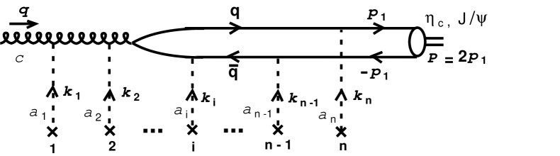
Figure 1: General amplitude for $\eta_{c}$ or $J/\psi$ production induced by $n$ scatterings off static centres $1,\ldots\,n$ located at $\vec{x}_{1},\ldots\,\vec{x}_{n}$. The static centres are ordered and labelled according to their increasing longitudinal position, and $\vec{k}_{i}$ is by definition the momentum transfered to the $q\bar{q}$ pair by centre # $i$. The color indices of the incident gluon and of the exchanged gluons are denoted by $c$ and $a_{i}$, respectively.

A QED illustration will define more precisely what we mean by ‘hard’ and ‘soft’ momentum transfers in this work. The Rutherford scattering $e+A\to e+A$ of a charged particle off a heavy nucleus is described by the Feynman diagram of Fig. 2a. Due to the Coulomb photon propagator the amplitude is proportional to $1/k_{\perp}^{2}$, where $k_{\perp}$ is the transverse momentum transfer. The cross section is then given by an infrared divergent integral, $\sigma\propto\int d^{2}\vec{k}_{\perp}/k_{\perp}^{4}$. For scattering on neutral atoms, the infrared cutoff is given by the inverse atomic radius $R$,

$$\mbox{$k_{\perp}$ is soft}\Longleftrightarrow k_{\perp}\sim\frac{1}{R}$$ (1.3)

On the other hand, in the pair creation process of Fig. 2b, $\gamma+A\to e^{+}e^{-}+A$, the scattering occurs off the neutral $e^{+}e^{-}$ pair. The amplitude is now proportional to the dipole moment $\propto 1/m_{e}$ of the pair, which introduces a factor $k_{\perp}/m_{e}$. The integral over momentum transfers is logarithmic, $\sigma\propto\int d^{2}\vec{k}_{\perp}/k_{\perp}^{2}$, and has support from an extended region,

$$\mbox{$k_{\perp}$ is hard}\Longleftrightarrow\frac{1}{R}\ll k_{\perp}\ll m_{e}$$ (1.4)

The electron mass sets the upper limit on the logarithmic integral. Indeed, for $k_{\perp}\gg m_{e}$ the virtual electron or positron in Fig. 2b is far off-shell, and the fermion propagator causes the integral to converge.

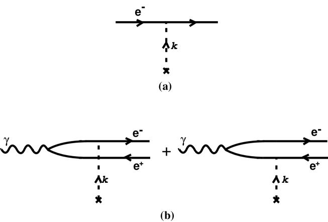
Figure 2: (a) Rutherford scattering of a charged particle off a nucleus. (b) Pair creation process $\gamma+A\to e^{+}e^{-}+A$.

The general classification of scattering into soft (monopole) and hard (dipole) exchange is not altered by effects due to a running of the coupling constant. In the following QCD analysis we shall thus for clarity assume a fixed coupling $\alpha_{s}$.

In the QCD process of Fig. 1, the incoming gluon has color charge, while the final charmonium is a color singlet. In analogy to the QED case above we may expect that the gluon will multiply Rutherford scatter, with the infrared cutoff provided by the inverse nucleon radius $R^{-1}\sim\Lambda_{QCD}$. At asymptotically large gluon energies the virtual $c\bar{c}$ pair travels a long distance, and it becomes highly probable that the pair is created far upstream of the target. Hence the multiple scattering in the target will actually occur off the quark pair rather than off the gluon. The compact pair is, however, created in a color octet state and it will behave like a gluon in soft rescattering processes.

On the other hand, it is intuitively plausible that a scattering which changes the color state of the pair (from singlet to octet or vice versa) will depend on the differing structure of quark pairs and gluons, ie, such a scattering will probe the dipole moment of the pair. As a consequence this scattering must be hard. This applies, in particular, to the last scattering in Fig. 1, which by definition changes the color state of the pair from octet to singlet.

In this paper we shall show explicitly how the above expectations are realized in QCD, and also find the answer to the questions mentioned in the beginning.

• Even though charge conjugation symmetry would allow the $J/\psi$ to be produced through one hard and one soft scattering in the target (without gluon emission), this would break the factorization between hard and soft processes. The soft exchange cannot be reliably calculated and such a contribution would in fact make it impossible to predict $J/\psi$ production in PQCD. We show that this problem does not arise since two hard scatterings are needed to produce a $J/\psi$.

• We shall also see that the broadening of $\langle p_{\perp}^{2}\rangle$ in nuclei does in fact depend on the hard scale, as suggested by the data of Eq. (1.2). Multiplying the differential cross section by a factor $p_{\perp}^{2}$ makes the integral sensitive to the upper cut-off, and $\langle p_{\perp}^{2}\rangle$ then depends (logarithmically) on the quark mass.

2 $\eta_{c}$ production

2.1 Single gluon exchange

The ¹S₀ $c\bar{c}$ state $\eta_{c}$ has positive charge conjugation and thus couples to two gluons – the projectile and one Coulomb gluon from the target as shown in Fig. 3.

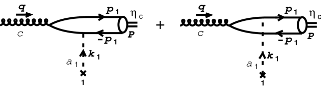
Figure 3: Amplitude for $\eta_{c}$ production induced by one scattering.

The amplitude for scattering from a fixed centre at position $\vec{x}_{1}$ is

$${\cal M}(gg\to\eta_{c}) = -\frac{R_{0}g^{3}}{\sqrt{4\pi m}}\frac{T^{a_{1}}_{A_{1}^{\prime}A_{1}}}{\sqrt{3}}\int\frac{d^{3}\vec{k}_{1}}{(2\pi)^{3}}(2\pi)^{3}\delta^{3}(\vec{q}+\vec{k}_{1}-2\vec{p}_{1})\frac{\exp(-i\vec{k}_{1}\cdot\vec{x}_{1})}{-\vec{k}_{1}^{2}}$$

$$\times \left({\cal A}_{1}+{\cal A}_{2}\right)$$

$${\cal A}_{1} = {\rm Tr}(T^{c}T^{a_{1}})\frac{{\rm Tr}\left[\parbox[b]{6.00006pt}{$\varepsilon$}\parbox[b]{5.50003pt}{ \raisebox{-0.86108pt}{$/$} }(-\parbox[b]{6.00006pt}{$p$}\parbox[b]{5.50003pt}{ \raisebox{-0.86108pt}{$/$} }_{1}+\parbox[b]{6.00006pt}{$k$}\parbox[b]{5.50003pt}{ \raisebox{-0.86108pt}{$/$} }_{1}+m)\gamma^{0}{{\cal P}_{S=0}}\right]}{(p_{1}-k_{1})^{2}-m^{2}+i\epsilon\,}$$

$${\cal A}_{2} = {\rm Tr}(T^{c}T^{a_{1}})\frac{{\rm Tr}\left[\gamma^{0}(\parbox[b]{6.00006pt}{$p$}\parbox[b]{5.50003pt}{ \raisebox{-0.86108pt}{$/$} }_{1}-\parbox[b]{6.00006pt}{$k$}\parbox[b]{5.50003pt}{ \raisebox{-0.86108pt}{$/$} }_{1}+m)\parbox[b]{6.00006pt}{$\varepsilon$}\parbox[b]{5.50003pt}{ \raisebox{-0.86108pt}{$/$} }{{\cal P}_{S=0}}\right]}{(p_{1}-k_{1})^{2}-m^{2}+i\epsilon\,}$$ (2.1)

Here the fixed centres are treated as heavy quarks of initial and final color charge $A_{1},A_{1}^{\prime}$. In the nonrelativistic limit of the charmonium bound state the momenta of the $c$ and $\bar{c}$ are the same, $p_{1}=p_{2}$, hence

$$q+k=2p_{1}\equiv P$$ (2.2)

where $k$ is the total momentum transfer to the target ($k=k_{1}$ in Fig. 3). The charm quark mass is denoted by $m$ and we have used the operator [24]

$${\cal P}_{S=0}=\frac{1}{\sqrt{2}}\gamma_{5}(\parbox[b]{6.00006pt}{$p$}\parbox[b]{5.50003pt}{ \raisebox{-0.86108pt}{$/$} }_{1}+m)$$ (2.3)

to project the $c\bar{c}$ pair onto the $\eta_{c}$ wave function at the origin, which is given by $R_{0}$. The incoming gluon polarization vector is denoted by $\varepsilon$.

The denominator in Eq. (2.1) is

$$(p_{1}-k_{1})^{2}-m^{2}=(q-p_{1})^{2}-m^{2}=-2p_{1}\cdot q=-q\cdot k$$ (2.4)

In the limit $q^{0}\to\infty$ and allowing the incoming gluon to have a finite transverse momentum, ie, $q\simeq(q^{0},\vec{q}_{\perp},q^{0}-q_{\perp}^{2}/2q^{0})$, we can write

$$(p_{1}-k_{1})^{2}-m^{2} \simeq -2m_{\perp}^{2}$$ (2.5)

$$k^{z} \simeq -\frac{2m_{\perp}^{2}+\vec{q}_{\perp}\cdot\vec{k}_{\perp}}{q^{0}}$$ (2.6)

$$m_{\perp}^{2} \equiv m^{2}+k_{\perp}^{2}/4$$ (2.7)

and obtain an expression for the $\eta_{c}$ production amplitude whose kinematics depends only on $\vec{k}_{1}$ (since $\vec{k}=\vec{k}_{1}$ here),

$${\cal M}(g(q)g(k_{1})\to\eta_{c}(2p_{1}))\simeq iq^{0}\frac{R_{0}g^{3}}{m_{\perp}^{2}\sqrt{24\pi m}}T^{c}_{A_{1}^{\prime}A_{1}}\frac{\exp(-i\vec{k}_{1\perp}\cdot\vec{x}_{1\perp})}{k_{1\perp}^{2}}\varepsilon_{0\mu\nu 3}\,\varepsilon^{\mu}\,k_{1}^{\nu}$$ (2.8)

where $\varepsilon_{\mu\nu\rho\sigma}$ is the fully antisymmetric Levi-Civita tensor. In the following, the direction of the incoming gluon will be chosen along the $z$-axis, ie, we take $\vec{q}_{\perp}=\vec{0}$ from now on.

We can now make the following observations.

• The $\eta_{c}$ production amplitude ${\cal M}(gg\to\eta_{c})$ is proportional to $\vec{k}_{1\perp}/k_{1\perp}^{2}$, ie, the effective values of $k_{1\perp}$ are hard,

  $$\Lambda_{QCD}\ll k_{1\perp}\ll m$$ (2.9)

  which justifies the use of perturbative QCD for this process.

• The fact that the effective upper limit of $k_{1\perp}$ is given by $m$ originates from the quark propagator, proportional to $1/m_{\perp}^{2}=1/(m^{2}+k_{1\perp}^{2}/4)$. As we shall see and as already announced in Eqs. (1.3) and (1.4), the $\vec{k}_{\perp}$ dependence of $m_{\perp}$ may be safely neglected when calculating amplitudes or cross sections. However, this dependence can be important in the calculation of other quantities, like $\langle{p_{\perp}^{2}}\rangle$ for $\eta_{c}$ or $J/\psi$, since weighting the differential cross section by $p_{\perp}^{2}$ can shift the effective values of the transverse momenta to be of order $m$. For this reason we will keep the $m_{\perp}$ dependence in the following.

• In this process, the incoming $c\bar{c}$ pair is in a color octet state, but $k_{1\perp}$ is not soft as it would have been in the case of elastic gluon scattering. In order to turn the color octet $c\bar{c}$ into a singlet the exchanged gluon has to probe the color dipole moment of the pair.

In the next subsection we consider the case when the $c\bar{c}$ pair undergoes two Coulomb scatterings in the target.

2.2 $\eta_{c}$ production through two gluon exchange

According to the notation of Fig. 1 we assume momentum transfers $\vec{k}_{1},\ \vec{k}_{2}$ from the two scattering centres located at $\vec{x}_{1},\ \vec{x}_{2}$, respectively. The longitudinal coordinates of the centres are taken to be $x_{1}^{z}=0,\ x_{2}^{z}=\tau>0$ (we do not consider double scattering from a single centre in this paper). The calculation, which is summarized below, shows the following.

• $k_{1\perp}$ is soft, whereas $k_{2\perp}$ is hard (in the sense of Eqs. (1.3) and (1.4)), ie,

  $$k_{1\perp}\sim\Lambda_{QCD};\ \ \ \ \ \Lambda_{QCD}\ll k_{2\perp}\ll m$$ (2.10)

• The amplitude factorizes. It is given by a convolution of the incoming gluon elastic scattering amplitude $gg\to g$ and the $\eta_{c}$ production amplitude $gg\to\eta_{c}$ given by Eq. (2.8),

  $$i{\cal M}(ggg\to\eta_{c}) = \sum_{\lambda^{\prime}}\int\frac{d^{2}\vec{k}_{1\perp}}{(2\pi)^{2}}i{\cal M}_{el}[g(q,\lambda)g(k_{1})\to g(q+k_{1},\lambda^{\prime})]\,\frac{1}{2q^{0}}$$ (2.11)

  $$\times i{\cal M}[g(q+k_{1},\lambda^{\prime})g(k_{2})\to\eta_{c}(q+k)]$$

  where $\lambda^{\prime}$ is the polarization of the intermediate gluon and

  $$i{\cal M}_{el}[g(q,\lambda)g(k_{1})\to g(q+k_{1},\lambda^{\prime})] = 2q^{0}g^{2}\varepsilon(\lambda)\cdot\varepsilon(\lambda^{\prime})f_{ca_{1}c^{\prime}}T^{a_{1}}_{A_{1}^{\prime}A_{1}}$$ (2.12)

  $$\times \frac{\exp(-i\vec{k}_{1\perp}\cdot\vec{x}_{1\perp})}{k_{1\perp}^{2}}$$

  This equation may be diagrammatically represented as

  $$\mbox{\raisebox{-31.2982pt}{\vbox{\epsfbox{figeq1a.eps}}}}=\sum_{\lambda^{\prime}}\int\frac{d^{2}\vec{k}_{1\perp}}{(2\pi)^{2}}\mbox{\raisebox{-28.45274pt}{\vbox{\epsfbox{figeq1b.eps}}}}\,\frac{1}{2q^{0}}\mbox{\raisebox{-28.45274pt}{\vbox{\epsfbox{figeq1c.eps}}}}$$ (2.13)

Let us now present the derivation of Eq. (2.11), which within our approach is exact in the limit $q^{0}\to\infty$. We write the amplitude as

$${\cal M}(ggg\to\eta_{c}) = -\frac{R_{0}g^{5}}{\sqrt{24\pi m}}T^{a_{1}}_{A_{1}^{\prime}A_{1}}T^{a_{2}}_{A_{2}^{\prime}A_{2}}\int\frac{d^{3}\vec{k}_{1}}{(2\pi)^{3}}\exp[i\tau(k^{z}_{1}-k^{z})]$$ (2.14)

$$\times \frac{\exp(-i\vec{k}_{1\perp}\cdot\vec{x}_{1\perp}-i\vec{k}_{2\perp}\cdot\vec{x}_{2\perp})}{k_{1\perp}^{2}\ k_{2\perp}^{2}}({\cal A+B})$$

where the amplitudes ${\cal A}$ (${\cal B}$) correspond to the 4 (8) diagrams shown in Fig. 4a (b).

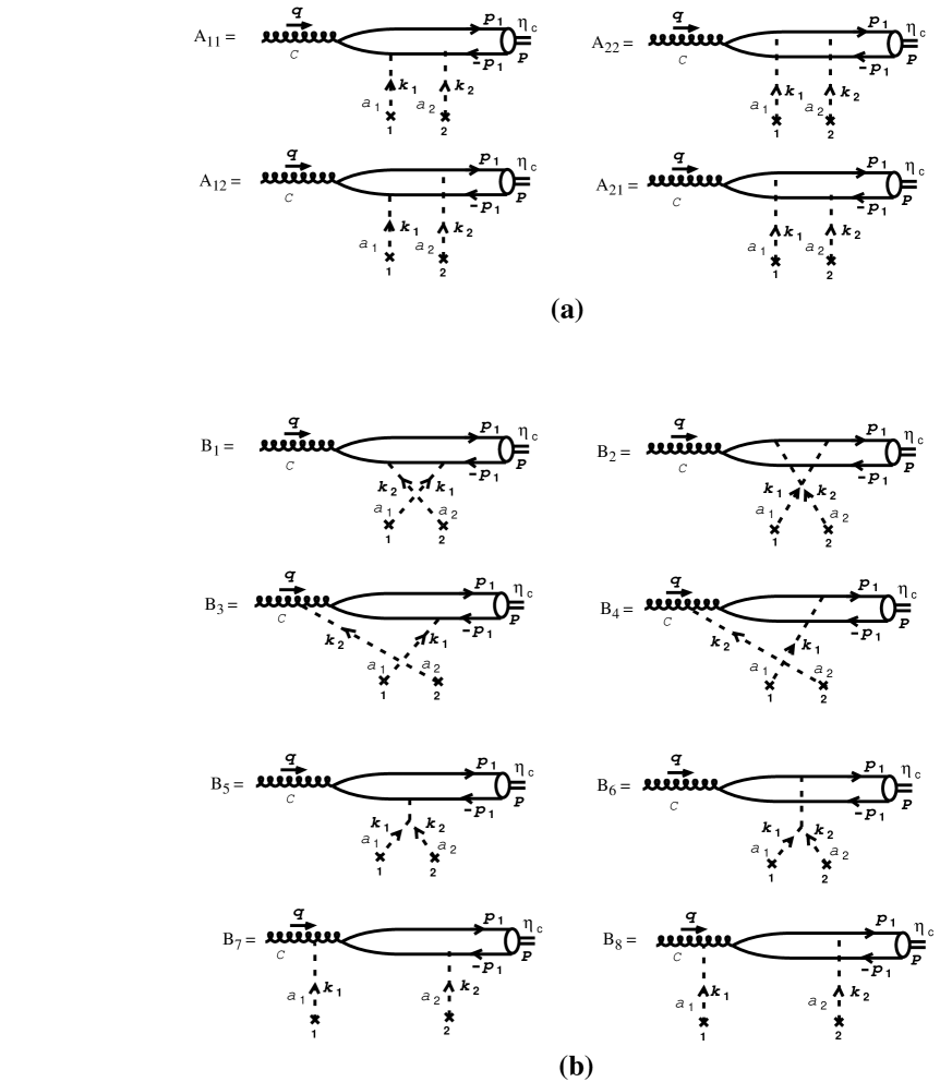
Figure 4: Diagrams for the $ggg\to\eta_{c}$ production amplitude.

Since we take $\tau>0$ the integral over $k_{1}^{z}$ can be evaluated by closing the integration contour in the upper half plane.

It is rather straightforward to see that none of the diagrams of Fig. 4b contribute in our limit, ie, ${\cal B}=0$. Namely,

• Since the Coulomb exchange is instantaneous, the diagrams $B_{1}\ldots B_{4}$ that have crossed exchanges involve the creation of $q\bar{q}$ pairs with energies $\propto q^{0}\to\infty$. All these diagrams have quark propagators whose residues in the Im $k^{z}_{1}>0$ plane vanish asymptotically.

• Diagrams $B_{5}$ and $B_{6}$ which involve the three-gluon vertex are also negligible. Our static scattering centres and the $q^{0}\to\infty$ limit restrict the Lorentz indices to be $\mu=\nu=0$ for the two gluons attached to the centres and $\sigma=0,3$ for the gluon attached to the $q\bar{q}$. Hence the vertex is at most on the order of the asymptotically vanishing longitudinal momentum transfers (cf Eqs. (2.6) and (2.23) below).

• In diagrams $B_{7}$ and $B_{8}$ the first rescattering gluon is attached to the projectile gluon. In the $q^{0}\to\infty$ limit the $g\to q\bar{q}$ fluctuation will occur long before the target, and thus such scattering should be suppressed. Technically this appears in the following way. The product of the gluon and quark propagators in diagrams $B_{7}$ and $B_{8}$ involves the denominator

  $$[(q+k_{1})^{2}+i\epsilon\,]\,[(p_{1}-k_{2})^{2}-m^{2}+i\epsilon\,]\simeq$$

  $$2(q^{0})^{2}\,[k^{z}_{1}+\frac{\vec{k}_{1\perp}^{2}}{2q^{0}}-i\epsilon\,]\,[k^{z}_{1}-k^{z}-\frac{\vec{k}_{1\perp}\cdot\vec{k}_{2\perp}}{q^{0}}-i\epsilon\,]\ \>,$$

  and thus has two poles in the upper $k^{z}_{1}$ half-plane, whose residues can easily be seen to cancel in the $q^{0}\to\infty$ limit.

Thus, only the four diagrams of Fig. 4a are nonvanishing and contribute to the ${\cal A}$-term in Eq. (2.14). Separating the color factors $c_{ij}$, the Lorentz traces ${\rm Tr}_{ij}$ and the denominators $\Delta_{ij}$ we write

$${\cal A}=\sum_{i,j}{A}_{ij}=\sum_{i,j}c_{ij}\frac{{\rm Tr}_{ij}}{\Delta_{ij}}$$ (2.15)

where

$$c_{11} = c_{12}={\rm Tr}(T^{c}T^{a_{1}}T^{a_{2}})$$

$$c_{22} = c_{21}={\rm Tr}(T^{c}T^{a_{2}}T^{a_{1}})$$ (2.16)

$${\rm Tr}_{11} = {\rm Tr}\left[\parbox[b]{6.00006pt}{$\varepsilon$}\parbox[b]{5.50003pt}{ \raisebox{-0.86108pt}{$/$} }(-\parbox[b]{6.00006pt}{$p$}\parbox[b]{5.50003pt}{ \raisebox{-0.86108pt}{$/$} }_{1}+\parbox[b]{6.00006pt}{$k$}\parbox[b]{5.50003pt}{ \raisebox{-0.86108pt}{$/$} }_{1}+\parbox[b]{6.00006pt}{$k$}\parbox[b]{5.50003pt}{ \raisebox{-0.86108pt}{$/$} }_{2}+m)\gamma^{0}(-\parbox[b]{6.00006pt}{$p$}\parbox[b]{5.50003pt}{ \raisebox{-0.86108pt}{$/$} }_{1}+\parbox[b]{6.00006pt}{$k$}\parbox[b]{5.50003pt}{ \raisebox{-0.86108pt}{$/$} }_{2}+m)\gamma^{0}(\parbox[b]{6.00006pt}{$p$}\parbox[b]{5.50003pt}{ \raisebox{-0.86108pt}{$/$} }_{1}-m)\gamma_{5}\right]$$

$${\rm Tr}_{22} = {\rm Tr}\left[\gamma^{0}(\parbox[b]{6.00006pt}{$p$}\parbox[b]{5.50003pt}{ \raisebox{-0.86108pt}{$/$} }_{1}-\parbox[b]{6.00006pt}{$k$}\parbox[b]{5.50003pt}{ \raisebox{-0.86108pt}{$/$} }_{2}+m)\gamma^{0}(\parbox[b]{6.00006pt}{$p$}\parbox[b]{5.50003pt}{ \raisebox{-0.86108pt}{$/$} }_{1}-\parbox[b]{6.00006pt}{$k$}\parbox[b]{5.50003pt}{ \raisebox{-0.86108pt}{$/$} }_{1}-\parbox[b]{6.00006pt}{$k$}\parbox[b]{5.50003pt}{ \raisebox{-0.86108pt}{$/$} }_{2}+m)\parbox[b]{6.00006pt}{$\varepsilon$}\parbox[b]{5.50003pt}{ \raisebox{-0.86108pt}{$/$} }(\parbox[b]{6.00006pt}{$p$}\parbox[b]{5.50003pt}{ \raisebox{-0.86108pt}{$/$} }_{1}-m)\gamma_{5}\right]$$

$${\rm Tr}_{12} = {\rm Tr}\left[\gamma^{0}(\parbox[b]{6.00006pt}{$p$}\parbox[b]{5.50003pt}{ \raisebox{-0.86108pt}{$/$} }_{1}-\parbox[b]{6.00006pt}{$k$}\parbox[b]{5.50003pt}{ \raisebox{-0.86108pt}{$/$} }_{2}+m)\parbox[b]{6.00006pt}{$\varepsilon$}\parbox[b]{5.50003pt}{ \raisebox{-0.86108pt}{$/$} }(-\parbox[b]{6.00006pt}{$p$}\parbox[b]{5.50003pt}{ \raisebox{-0.86108pt}{$/$} }_{1}+\parbox[b]{6.00006pt}{$k$}\parbox[b]{5.50003pt}{ \raisebox{-0.86108pt}{$/$} }_{1}+m)\gamma^{0}(\parbox[b]{6.00006pt}{$p$}\parbox[b]{5.50003pt}{ \raisebox{-0.86108pt}{$/$} }_{1}-m)\gamma_{5}\right]$$

$${\rm Tr}_{21} = {\rm Tr}\left[\gamma^{0}(\parbox[b]{6.00006pt}{$p$}\parbox[b]{5.50003pt}{ \raisebox{-0.86108pt}{$/$} }_{1}-\parbox[b]{6.00006pt}{$k$}\parbox[b]{5.50003pt}{ \raisebox{-0.86108pt}{$/$} }_{1}+m)\parbox[b]{6.00006pt}{$\varepsilon$}\parbox[b]{5.50003pt}{ \raisebox{-0.86108pt}{$/$} }(-\parbox[b]{6.00006pt}{$p$}\parbox[b]{5.50003pt}{ \raisebox{-0.86108pt}{$/$} }_{1}+\parbox[b]{6.00006pt}{$k$}\parbox[b]{5.50003pt}{ \raisebox{-0.86108pt}{$/$} }_{2}+m)\gamma^{0}(\parbox[b]{6.00006pt}{$p$}\parbox[b]{5.50003pt}{ \raisebox{-0.86108pt}{$/$} }_{1}-m)\gamma_{5}\right]$$ (2.17)

$$\Delta_{11} = \Delta_{22}=[(p_{1}-k)^{2}-m^{2}+i\epsilon\,][(p_{1}-k_{2})^{2}-m^{2}+i\epsilon\,]$$

$$\Delta_{12} = \Delta_{21}=[(p_{1}-k_{1})^{2}-m^{2}+i\epsilon\,][(p_{1}-k_{2})^{2}-m^{2}+i\epsilon\,]$$ (2.18)

Reversing the order of the $\gamma$-matrices in ${\rm Tr}_{22}$ and ${\rm Tr}_{21}$ one easily finds

$${\rm Tr}_{11}=-{\rm Tr}_{22}\ ;\ \ \ \ {\rm Tr}_{12}=-{\rm Tr}_{21}$$ (2.19)

In QED Eq. (2.19) ensures a vanishing transition amplitude between a three-photon state (of negative charge conjugation, $C=-$) and a ¹S₀ positronium state $(C=+)$. Due to the color charges of QCD the analogous amplitude does not vanish but is proportional to the fully antisymmetric structure constants $f_{abc}$ of SU(3),

$${\cal A} = \left[{\rm Tr}(T^{c}T^{a_{1}}T^{a_{2}})-{\rm Tr}(T^{c}T^{a_{2}}T^{a_{1}})\right]\left[\frac{{\rm Tr}_{11}}{\Delta_{11}}+\frac{{\rm Tr}_{12}}{\Delta_{12}}\right]$$ (2.20)

$$= \frac{i}{2}f_{ca_{1}a_{2}}\left[\frac{{\rm Tr}_{11}}{\Delta_{11}}+\frac{{\rm Tr}_{12}}{\Delta_{12}}\right]$$

An evaluation of the traces gives, in the $q^{0}\to\infty$ limit,

$${\rm Tr}_{11} = -2i(q^{0})^{2}\,\varepsilon_{0\mu\nu 3}\,\varepsilon^{\mu}\,(k_{1}+k_{2})^{\nu}$$

$${\rm Tr}_{12} = -2i(q^{0})^{2}\,\varepsilon_{0\mu\nu 3}\,\varepsilon^{\mu}\,(-k_{1}+k_{2})^{\nu}\ \>.$$ (2.21)

The denominators may be simplified using

$$(p_{1}-k_{1})^{2}-m^{2}+i\epsilon\, \simeq q^{0}\,(k^{z}_{1}+\frac{\vec{k}_{1\perp}\cdot\vec{k}_{2\perp}}{q^{0}}+i\epsilon\,)$$

$$(p_{1}-k_{2})^{2}-m^{2}+i\epsilon\, \simeq -q^{0}\,(k^{z}_{1}-k^{z}-\frac{\vec{k}_{1\perp}\cdot\vec{k}_{2\perp}}{q^{0}}-i\epsilon\,)\>.$$ (2.22)

Integrating over $k^{z}_{1}$ in Eq. (2.14) by closing the contour in the upper half-plane picks according to Eq. (2.22) the pole

$$k^{z}_{1}=k^{z}+\frac{\vec{k}_{1\perp}\cdot\vec{k}_{2\perp}}{q^{0}}+i\epsilon\,$$ (2.23)

such that

$$\int\frac{dk^{z}_{1}}{2\pi}\,{\cal A}\,\exp[i\tau(k^{z}_{1}-k^{z})] = i(q^{0})^{2}f_{ca_{1}a_{2}}\varepsilon_{0\mu\nu 3}\varepsilon^{\mu}$$ (2.24)

$$\times \left[\frac{(k_{1}+k_{2})^{\nu}}{q^{0}k^{z}(-q^{0})}+\frac{(-k_{1}+k_{2})^{\nu}}{(-q^{0})(q^{0}k^{z}+2\vec{k}_{1\perp}\cdot\vec{k}_{2\perp})}\right]\hskip 28.45274pt$$

Note that the poles of the Coulomb gluon propagators lead to a subleading contribution in the $q_{0}\to\infty$ limit. Using Eq. (2.6) for $\vec{q}_{\perp}=\vec{0}$ and

$$|\vec{k}_{1\perp}\cdot\vec{k}_{2\perp}|\ll m_{\perp}^{2}$$ (2.25)

we find for the full amplitude of Eq. (2.14)

$${\cal M}(ggg\to\eta_{c}) = -iq^{0}\frac{R_{0}g^{5}}{m_{\perp}^{2}\sqrt{24\pi m}}T^{a_{1}}_{A_{1}^{\prime}A_{1}}T^{a_{2}}_{A_{2}^{\prime}A_{2}}f_{ca_{1}a_{2}}\,\varepsilon_{0\mu\nu 3}\,\varepsilon^{\mu}$$ (2.26)

$$\times \int\frac{d^{2}\vec{k}_{1\perp}}{(2\pi)^{2}}\exp(-i\vec{k}_{1\perp}\cdot\vec{x}_{1\perp}-i\vec{k}_{2\perp}\cdot\vec{x}_{2\perp})\frac{1}{k_{1\perp}^{2}}\frac{k_{2}^{\nu}}{k_{2\perp}^{2}}$$

Writing

$$\varepsilon^{\mu}(\lambda)=-\sum_{\lambda^{\prime}}\left[\varepsilon(\lambda)\cdot\varepsilon(\lambda^{\prime})^{*}\right]\varepsilon^{\mu}(\lambda^{\prime})$$ (2.27)

directly leads to the factorized expression of Eq. (2.11).

Let us note that Eq. (2.26) involves the denominator $m_{\perp}^{2}=m^{2}+(\vec{k}_{1\perp}+\vec{k}_{2\perp})^{2}/4$, instead of $(m^{2}+\vec{k}_{2\perp}^{\ 2}/4)$ for the $\eta_{c}$ production amplitude contained in Eq. (2.11). By calculating ${\cal M}(ggg\to\eta_{c})$ as a function of $\vec{k}_{\perp}$ and $\vec{x}_{2\perp}-\vec{x}_{1\perp}$, one shows that the effective values of the transverse momenta satisfy $k_{1\perp}\ll k_{2\perp}\sim k_{\perp}$ for all $|\vec{x}_{2\perp}-\vec{x}_{1\perp}|$ (provided $k_{\perp}\gg\Lambda_{QCD}$), so that Eq. (2.11) follows. However, as mentioned earlier the $\vec{k}_{1\perp}$ dependence of $m_{\perp}$ can be important when calculating $\langle{p_{\perp}^{2}}\rangle$, for which the correct expression to start with will be Eq. (2.26).

The $\vec{k}_{2\perp}$ factor in Eq. (2.26) explicitly shows that the second exchange is hard in the sense of Eq. (1.4). The amplitude to turn the color octet $c\bar{c}$ pair into a color singlet is thus proportional to the dipole moment of the pair. In the next section we study the analogous situation in $J/\psi$ production, which differs from the case of the $\eta_{c}$ since a minimum of two exchanges with the target is now required.

3 $J/\psi$ production

3.1 Two gluon exchange

The $J/\psi$ is a ³S₁ charmonium state with negative charge conjugation, and hence couples to a minimum of three gluons. The lowest order amplitude (which does not involve gluons in the final state) is thus given by the diagrams of Fig. 4a, with the $\eta_{c}$ replaced by the $J/\psi$. For the reasons discussed in the previous section the diagrams $B_{1}$ and $B_{2}$ of Fig. 4b do not contribute to high energy $J/\psi$ production. Hence the amplitude may again be written as in Eq. (2.14) with ${\cal B}=0$. In the expression for ${\cal A}$, the only difference is that the projection operator (2.3) is replaced by a projection onto a vector state [24],

$${\cal P}_{S=1}=-\frac{1}{\sqrt{2}}\parbox[b]{6.00006pt}{$e$}\parbox[b]{5.50003pt}{ \raisebox{-0.86108pt}{$/$} }(\parbox[b]{6.00006pt}{$p$}\parbox[b]{5.50003pt}{ \raisebox{-0.86108pt}{$/$} }_{1}+m)$$ (3.1)

where $e(S_{z})$ is the $J/\psi$ polarization vector, defined in the $J/\psi$ rest frame as

$$e(S_{z}=\pm 1) \equiv e_{T}=(0,1,\pm i,0)/\sqrt{2}\ \ \ \ \mbox{{\rm for transverse }}J/\psi\$$

$$e(S_{z}=0) \equiv e_{L}=(0,\vec{0}_{\perp},1)\ \ \ \ \ \ \ \ \ \ \ \ \mbox{{\rm for longitudinal }}J/\psi\$$ (3.2)

We shall use the Gottfried-Jackson frame, where the $z$-axis in the $J/\psi$ rest frame is taken parallel to the projectile momentum $\vec{q}$. The invariant product $e\cdot w$ for any vector $w$ can then be expressed, in the high energy limit we consider, as

$$e_{T}\cdot w = -\vec{e}_{\perp}\cdot\vec{w}_{\perp}$$

$$e_{L}\cdot w = m\frac{q\cdot w}{q\cdot p_{1}}-\frac{p_{1}\cdot w}{m}$$ (3.3)

From the trace expressions corresponding to Eq. (2.17) it can be seen that for the $J/\psi$ amplitude

$${\rm Tr}_{11}={\rm Tr}_{22}\ ;\ \ \ \ {\rm Tr}_{12}={\rm Tr}_{21}$$ (3.4)

which differ from the $\eta_{c}$ case of Eq. (2.19) by a sign. It is in fact easily seen that Eq. (3.4) for the $J/\psi$ generalizes in the case of $n$ scatterings to

$${\rm Tr}_{A}=(-1)^{n}\,{\rm Tr}_{A^{*}}$$ (3.5)

where $A$ and $A^{*}$ are charge conjugated diagrams. Eq. (3.5) is readily understood as a consequence of charge conjugation invariance in QED.

The expression for the amplitude ${\cal A}$ in Eq. (2.14) for $J/\psi$ production is then

$${\cal A} = \left[{\rm Tr}(T^{c}T^{a_{1}}T^{a_{2}})+{\rm Tr}(T^{c}T^{a_{2}}T^{a_{1}})\right]\left[\frac{{\rm Tr}_{11}}{\Delta_{11}}+\frac{{\rm Tr}_{12}}{\Delta_{12}}\right]$$ (3.6)

$$= \frac{1}{2}d_{ca_{1}a_{2}}\left[\frac{{\rm Tr}_{11}}{\Delta_{11}}+\frac{{\rm Tr}_{12}}{\Delta_{12}}\right]$$

In the limit $q^{0}\to\infty$ the explicit expressions for the traces are

$${\rm Tr}_{11}=-{\rm Tr}_{12}=-4m(q^{0})^{2}\beta_{T,L}(\lambda)$$ (3.7)

where $\beta$ depends on the polarization $(\lambda)$ of the incoming gluon and on that of the $J/\psi$ $(T,L)$,

$$\beta_{T}(\lambda) = -\varepsilon(\lambda)\cdot e_{T}$$

$$\beta_{L}(\lambda) = 2\varepsilon(\lambda)\cdot p_{1}\,m/m_{\perp}^{2}$$ (3.8)

For the general case of $n$ scatterings (cf Fig. 1) the trace for a given diagram is

$${\rm Tr}=-4m(q^{0})^{n}\beta_{T,L}(\lambda)(-1)^{n_{\bar{q}}}$$ (3.9)

where $n_{\bar{q}}$ is the number of Coulomb gluons attached to the antiquark.

Using now Eqs. (3.6) and (3.7) in the expression (2.14) and performing the $k^{z}_{1}$-integral by picking up the pole (2.23) we find (once again $|\vec{k}_{1\perp}\cdot\vec{k}_{2\perp}|\ll m_{\perp}^{2}$),

$${\cal M}(g(\lambda)gg\to J/\psi) = -iq^{0}m\frac{R_{0}g^{5}}{m_{\perp}^{4}\sqrt{24\pi m}}T^{a_{1}}_{A_{1}^{\prime}A_{1}}T^{a_{2}}_{A_{2}^{\prime}A_{2}}d_{ca_{1}a_{2}}\beta_{T,L}(\lambda)\hskip 28.45274pt$$ (3.10)

$$\times \int\frac{d^{2}\vec{k}_{1\perp}}{(2\pi)^{2}}\exp(-i\vec{k}_{1\perp}\cdot\vec{x}_{1\perp}-i\vec{k}_{2\perp}\cdot\vec{x}_{2\perp})\frac{\vec{k}_{1\perp}\cdot\vec{k}_{2\perp}}{k_{1\perp}^{2}\,k_{2\perp}^{2}}\hskip 28.45274pt$$

Since the numerator of the $J/\psi$ production amplitude (3.10) is proportional to $\vec{k}_{1\perp}$ and $\vec{k}_{2\perp}$ it follows that both transferred momenta are hard in the sense of Eq. (1.4). This contribution to $J/\psi$ production is then a higher twist effect compared to the standard one involving a single target scattering and a radiated gluon, as is required by factorization between hard and soft processes in PQCD.

Next we shall investigate the case of one ‘extra’ target scattering. This is of importance for understanding the general systematics of rescattering effects in $J/\psi$ production and the ${p_{\perp}}$-broadening effects in nuclei.

3.2 Three gluon exchange in $J/\psi$ production

In the high energy limit the $J/\psi$ production amplitude induced by three scatterings on static centres is given by the eight diagrams of Fig. 5.

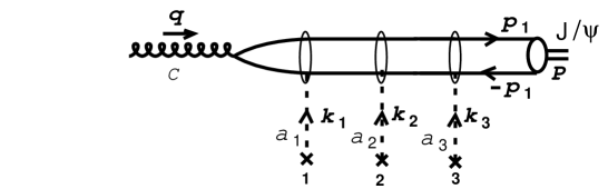
Figure 5: $J/\psi$ production amplitude induced by three scatterings. Eight diagrams are generated by attaching each Coulomb gluon to one of the quark lines.

From the $\eta_{c}$ result (2.26) we may expect that the last transfer $(k_{3})$, which turns the $c\bar{c}$ pair into a color singlet, will be hard. It is less obvious if either one of the first two exchanges can be soft. As already noticed, the propagating quark pair stays dominantly in a color octet state even when undergoing a hard scattering (except for the last one). Therefore, one would expect it to suffer soft rescattering both before and after the first hard exchange. This is indeed what we shall find below.

Taking $x_{1}^{z}=0,\ x_{2}^{z}=\tau$ and $x_{3}^{z}=\tau^{\prime}>\tau>0$ the amplitude can be expressed as

$${\cal M} = -\frac{R_{0}g^{7}}{\sqrt{24\pi m}}\int\frac{d^{3}\vec{k}_{1}}{(2\pi)^{3}}\frac{d^{3}\vec{k}_{2}}{(2\pi)^{3}}\prod_{j=1}^{3}\left[T^{a_{j}}_{A_{j}^{\prime}A_{j}}\frac{\exp(-i\vec{k}_{j\perp}\cdot\vec{x}_{j\perp})}{k_{j\perp}^{2}}\right]$$ (3.11)

$$\times \exp\left[-ik^{z}\tau^{\prime}+ik^{z}_{1}\tau^{\prime}+ik^{z}_{2}(\tau^{\prime}-\tau)\right]{\cal A}$$

After some algebra we find, with an obvious notation for color traces,

$${\cal A} = 4m(q^{0})^{3}\beta_{T,L}(\lambda)\left\{\left[{\rm Tr}(ca_{1}a_{2}a_{3})-{\rm Tr}(a_{1}ca_{3}a_{2})\right]\left(\frac{1}{\Delta_{1}}-\frac{1}{\Delta_{5}}\right)\right.$$ (3.12)

$$+ \left.\left[{\rm Tr}(a_{1}ca_{2}a_{3})-{\rm Tr}(ca_{1}a_{3}a_{2})\right]\left(\frac{1}{\Delta_{7}}-\frac{1}{\Delta_{3}}\right)\right\}$$

where

$$\Delta_{1} = [(p_{1}-q)^{2}-m^{2}+i\epsilon\,][(p_{1}-k_{2}-k_{3})^{2}-m^{2}+i\epsilon\,][(p_{1}-k_{3})^{2}-m^{2}+i\epsilon\,]$$

$$\Delta_{5} = [(p_{1}-k_{1}-k_{2})^{2}-m^{2}+i\epsilon\,][(p_{1}-k_{2})^{2}-m^{2}+i\epsilon\,][(p_{1}-k_{3})^{2}-m^{2}+i\epsilon\,]$$

$$\Delta_{3} = [(p_{1}-k_{1})^{2}-m^{2}+i\epsilon\,][(p_{1}-k_{2}-k_{3})^{2}-m^{2}+i\epsilon\,][(p_{1}-k_{3})^{2}-m^{2}+i\epsilon\,]$$

$$\Delta_{7} = [(p_{1}-k_{2})^{2}-m^{2}+i\epsilon\,][(p_{1}-k_{1}-k_{3})^{2}-m^{2}+i\epsilon\,][(p_{1}-k_{3})^{2}-m^{2}+i\epsilon\,]$$

In the $q^{0}\to\infty$ limit we have

$$(p_{1}-q)^{2}-m^{2} \simeq -2m_{\perp}^{2}$$

$$(p_{1}-k_{i})^{2}-m^{2}+i\epsilon\, \simeq q^{0}[k^{z}_{i}+\vec{k}_{i\perp}\cdot(\vec{k}_{j\perp}+\vec{k}_{k\perp})/q^{0}+i\epsilon\,]$$

$$(p_{1}-k_{i}-k_{j})^{2}-m^{2}+i\epsilon\, \simeq q^{0}[k^{z}_{i}+k^{z}_{j}+\vec{k}_{k\perp}\cdot(\vec{k}_{i\perp}+\vec{k}_{j\perp})/q^{0}+i\epsilon\,]$$ (3.14)

where $i,j,k$ is any cyclic combination of $1,2,3$. Integrating over $k^{z}_{2}$ and then over $k^{z}_{1}$ picks the poles

$$k^{z}_{2}=k^{z}-k^{z}_{1}+(\vec{k}_{1\perp}+\vec{k}_{2\perp})\cdot\vec{k}_{3\perp}/q^{0}+i\epsilon\,$$ (3.15)

and

$$k^{z}_{1} = k^{z}+\vec{k}_{1\perp}\cdot(\vec{k}_{2\perp}+\vec{k}_{3\perp})/q^{0}+i\epsilon\,$$

$$k^{z}_{1} = k^{z}+\vec{k}_{1\perp}\cdot(\vec{k}_{2\perp}+\vec{k}_{3\perp})/q^{0}+2\vec{k}_{2\perp}\cdot\vec{k}_{3\perp}/q^{0}+i\epsilon\,$$ (3.16)

As in the cases previously studied, the first longitudinal transfer $k^{z}_{1}\simeq k^{z}$ puts the $c\bar{c}$ pair on-shell, while the succeeding transfers $k^{z}_{i}\ll k^{z}$ maintain this on-shellness. This is because

$$|\vec{k}_{i\perp}\cdot\vec{k}_{j\perp}|\ll m_{\perp}^{2}$$ (3.17)

holds in both relevant ranges (1.3) and (1.4). We finally obtain

$${\cal M}(4g\to J/\psi) = imq^{0}\frac{R_{0}g^{7}}{m_{\perp}^{4}\sqrt{24\pi m}}\beta_{T,L}(\lambda)\hskip 113.81102pt$$ (3.18)

$$\times \int\frac{d^{2}\vec{k}_{1}}{(2\pi)^{2}}\frac{d^{2}\vec{k}_{2}}{(2\pi)^{2}}\prod_{j=1}^{3}\left[T^{a_{j}}_{A_{j}^{\prime}A_{j}}\,\frac{\exp(-i\vec{k}_{j\perp}\cdot\vec{x}_{j\perp})}{k_{j\perp}^{2}}\right]$$

$$\times \left(d_{ca_{1}d}f_{a_{2}a_{3}d}\,\vec{k}_{1\perp}\cdot\vec{k}_{3\perp}+f_{ca_{1}d}d_{a_{2}a_{3}d}\,\vec{k}_{2\perp}\cdot\vec{k}_{3\perp}\right)$$

From Eq. (3.18) we deduce the following:

• The last momentum transfer $k_{3}$ is hard.

• One of the first two transfers is hard and the other is soft.

Let us consider the two parts of the amplitude (3.18) separately,

$${\cal M}={\cal M}_{1}+{\cal M}_{2}$$ (3.19)

where the index indicates which is the first hard transfer. It is straightforward to see that the ${\cal M}_{2}$ part factorizes in a way analogous to Eq. (2.11),

$$i{\cal M}_{2} = \sum_{\lambda^{\prime}}\int\frac{d^{2}\vec{k}_{1\perp}}{(2\pi)^{2}}i{\cal M}_{el}[g(q,\lambda)g(k_{1})\to g(q+k_{1},\lambda^{\prime})]\,\frac{1}{2q^{0}}$$ (3.20)

$$\times i{\cal M}[g(q+k_{1},\lambda^{\prime})g(k_{2})g(k_{3})\to J/\psi(q+k)]$$

or in pictorial form

$$\mbox{\raisebox{-31.2982pt}{\vbox{\epsfbox{figeq2a.eps}}}}=\sum_{\lambda^{\prime}}\int\frac{d^{2}\vec{k}_{1\perp}}{(2\pi)^{2}}\mbox{\raisebox{-25.6073pt}{\vbox{\epsfbox{figeq2b.eps}}}}\,\frac{1}{2q^{0}}\mbox{\raisebox{-28.45274pt}{\vbox{\epsfbox{figeq2c.eps}}}}$$ (3.21)

The soft transfer $k_{1\perp}$ thus mimics rescattering of the initial gluon. (As remarked above, however, the longitudinal part $k^{z}_{1}$ is relatively big in the sense that it puts the incoming heavy quark pair on its mass-shell, as seen from Eq. (3.16).)

Factorization is somewhat more involved for the ${\cal M}_{1}$ term of Eq. (3.19), where $k_{1\perp}$ is hard. A relation like

$$\mbox{\raisebox{-31.2982pt}{\vbox{\epsfbox{figeq3a.eps}}}}=\sum_{\lambda^{\prime}}\int\frac{d^{2}\vec{k}_{2\perp}}{(2\pi)^{2}}\mbox{\raisebox{-25.6073pt}{\vbox{\epsfbox{figeq3b.eps}}}}\,\frac{1}{2q^{0}}\mbox{\raisebox{-28.45274pt}{\vbox{\epsfbox{figeq3c.eps}}}}$$ (3.22)

cannot hold, since the soft $k_{2\perp}$ exchange sees a color which has been ‘rotated’ away from the incoming color $c$ by the $k_{1}$ gluon. Rather, the color structure of the ${\cal M}_{1}$ term in Eq. (3.18) can be pictorially represented as

                               $$(i{\cal M}_{1})_{color}=d_{ca_{1}d}\,if_{a_{2}a_{3}d}$$ (3.23)

$$=\ \mbox{\raisebox{-28.45274pt}{\vbox{\epsfbox{figeq4.eps}}}}$$

On the other hand, forgetting the color factors and considering only the Lorentz structure of ${\cal M}_{1}$, we easily see from Eq. (3.18) the validity of the factorization formula

             $$(i{\cal M}_{1})_{Lorentz}=\mbox{\raisebox{-28.45274pt}{\vbox{\epsfbox{figeq5a.eps}}}}$$ (3.24)

$$=\sum_{\lambda^{\prime}}\int\frac{d^{2}\vec{k}_{2\perp}}{(2\pi)^{2}}\ \ \ \ \mbox{\raisebox{-28.45274pt}{\vbox{\epsfbox{figeq5b.eps}}}}\,\frac{1}{2q^{0}}\ \ \ \ \mbox{\raisebox{-31.2982pt}{\vbox{\epsfbox{figeq5c.eps}}}}$$

The differing structure of Eqs. (3.23) and (3.24) prevents us from factorizing the ${\cal M}_{1}$ part of the amplitude in a straightforward way analogous to Eq. (3.20) for ${\cal M}_{2}$. The soft gluon $(k_{2})$ between the hard transfers $(k_{1},k_{3})$ changes the color structure of the hard production amplitude and, as we shall see below, ensures that there is no interference in the cross section between ${\cal M}_{1}$ and ${\cal M}_{2}$. It is convenient to summarize our result for the full amplitude (3.18) in the form

$${\cal M}(4g\to J/\psi) = {\cal M}_{1}+{\cal M}_{2}$$ (3.25)

$$= \prod_{j=1}^{3}\left[T^{a_{j}}_{A_{j}^{\prime}A_{j}}\right]\left(if_{a_{2}a_{3}d}d_{ca_{1}d}\widetilde{\cal M}_{1}+if_{ca_{1}d}d_{a_{2}a_{3}d}\widetilde{\cal M}_{2}\right)$$

where $\widetilde{\cal M}_{i}=({\cal M}_{i})_{Lorentz}$. For instance, Eq. (3.24) is explicitly

$$i\widetilde{\cal M}_{1} = \sum_{\lambda^{\prime}}\int\frac{d^{2}\vec{k}_{2\perp}}{(2\pi)^{2}}i\widetilde{\cal M}_{el}[g(q,\lambda)g(k_{2})\to g(q+k_{2},\lambda^{\prime})]\,\frac{1}{2q^{0}}$$ (3.26)

$$\times i\widetilde{\cal M}[g(q+k_{2},\lambda^{\prime})g(k_{1})g(k_{3})\to J/\psi(q+k)]$$

where

$$\widetilde{\cal M}_{el}[g(q,\lambda)g(k_{2})\to g(q+k_{2},\lambda^{\prime})]\hskip 156.49014pt$$

$$\hskip 56.9055pt=2q^{0}\,g^{2}\,[-\varepsilon(\lambda)\cdot\varepsilon(\lambda^{\prime})]\frac{\exp(-i\vec{k}_{2\perp}\cdot\vec{x}_{2\perp})}{k_{2\perp}^{2}}$$

$$\widetilde{\cal M}[g(q+k_{2},\lambda^{\prime})g(k_{1})g(k_{3})\to J/\psi(q+k)]\hskip 113.81102pt$$

$$=-imq^{0}\frac{R_{0}g^{5}}{m_{\perp}^{4}\sqrt{24\pi m}}\beta_{T,L}(\lambda^{\prime})\hskip 56.9055pt$$

$$\times\int\frac{d^{2}\vec{k}_{1}}{(2\pi)^{2}}\exp(-i\vec{k}_{1\perp}\cdot\vec{x}_{1\perp}-i\vec{k}_{3\perp}\cdot\vec{x}_{3\perp})\frac{\vec{k}_{1\perp}\cdot\vec{k}_{3\perp}}{k_{1\perp}^{2}\,k_{3\perp}^{2}}$$ (3.27)

4 Cross sections and $p_{\perp}$-broadening

In this section we derive the expressions for the production cross sections and $\langle{p_{\perp}^{2}}\rangle$ of the $\eta_{c}$ and $J/\psi$ bound states, based on the amplitudes found in the previous sections.

The differential cross section for scattering on static centres is

$$\frac{d^{2}\sigma_{n}}{d^{2}\vec{P}_{\perp}}=\frac{1}{(2\pi)^{2}(2q^{0})^{2}}\left\langle\left|{\cal M}_{n}\right|^{2}\right\rangle\ ,$$ (4.1)

where ${\cal M}_{n}$ is the bound state production amplitude induced by $n$ scatterings $(n\geq 1)$ and $\vec{P}_{\perp}=2\vec{p}_{1\perp}$. In addition to the implicit color/spin summation and averaging, the average sign in Eq. (4.1) denotes an average over positions of the scattering centres.

In the case of one scattering centre, and assuming a uniform distribution of this centre with a constant volume density $\rho$, our description is equivalent to the standard infinite momentum frame description with a gluon distribution $\propto 1/x$ (see Appendix A). For $n>1$ centres we assume in the following that the centres are distributed independently with the same constant density $\rho$. Thus the average of Eq. (4.1) is defined to be

$$\left\langle{\left|{\cal M}_{n}\right|}^{2}\right\rangle\equiv\int\prod_{i=1}^{n}(\rho\,d^{3}\vec{x}_{i})\,\overline{\left|{\cal M}_{n}\right|^{2}}$$ (4.2)

where the overline indicates the remaining color/spin sum and average. We also define the volume, transverse area and length of the target by

$$V = \int d^{3}\vec{x}_{i}$$

$$S = \int d^{2}\vec{x}_{i\perp}$$

$$L = \int dx_{i}^{z}$$ (4.3)

Our approach can in principle also deal with a case of correlated centres, which might be of phenomenological relevance, as discussed in the final section.

From Eq. (4.1) we obtain the $\langle{P_{\perp}^{2}}\rangle$ induced by $n$ scatterings as

$$\langle{P_{\perp}^{2}}\rangle_{n}=\frac{\int d^{2}\vec{P}_{\perp}\,\,\vec{P}_{\perp}^{2}\,d^{2}\sigma_{n}/d^{2}\vec{P}_{\perp}}{\int d^{2}\vec{P}_{\perp}\,d^{2}\sigma_{n}/d^{2}\vec{P}_{\perp}}$$ (4.4)

4.1 $\eta_{c}$ production

One scattering

We first give the cross section for the basic single gluon exchange process. Squaring the amplitude ${\cal M}(gg\to\eta_{c})$ of Eq. (2.8) and using $\varepsilon=(0,1,\pm i,0)/\sqrt{2}$ for the projectile gluon polarization states we obtain

$$\frac{d\sigma_{1}}{dP_{\perp}^{2}}=\frac{4\pi}{9}\rho V\frac{R_{o}^{2}\alpha_{s}^{3}}{M(P_{\perp}^{2}+M^{2})^{2}P_{\perp}^{2}}\ ,$$ (4.5)

where $M=2m$ and the factor $\rho V$ arises from the trivial averaging over $\vec{x}_{1}$. Integrating over $P_{\perp}^{2}$ yields

$$\sigma_{1}=\frac{4\pi}{9}\rho V\frac{R_{o}^{2}\alpha_{s}^{3}}{M^{5}}\log\left(\frac{M^{2}}{\Lambda_{QCD}^{2}}\right)\ .$$ (4.6)

Two scatterings

For the production process induced by two scatterings we use the convolution formula of Eq. (2.11), which as we now shall show implies a similar convolution at the level of the cross section,

$$\frac{d^{2}\sigma_{2}}{d^{2}\vec{P}_{\perp}}=\int d^{2}\vec{k}_{1\perp}\left[\frac{d^{2}{\cal P}_{el}}{d^{2}\vec{k}_{1\perp}}\right]_{1}\,\frac{d^{2}\sigma_{1}(\vec{P}_{\perp}-\vec{k}_{1\perp})}{d^{2}\vec{P}_{\perp}}$$ (4.7)

The first factor is the probability density for gluon elastic scattering off the first static centre. Thus $d^{2}\sigma_{2}/d^{2}\vec{P}_{\perp}$ is given by a convolution of the probability for having a gluon elastic scattering of transfer $\vec{k}_{1\perp}$ first and the differential cross section for the basic production process with a single scattering of momentum transfer $\vec{P}_{\perp}-\vec{k}_{1\perp}$ occurring thereafter.

To derive Eq. (4.7) we express the elastic gluon and $\eta_{c}$ production amplitude in the form

$$i{\cal M}_{el}[g(q,\lambda)g(k_{1})\to g(q+k_{1},\lambda^{\prime})] = f_{ca_{1}c^{\prime}}T_{A_{1}^{\prime}A_{1}}^{a_{1}}\exp(-i\vec{k}_{1\perp}\cdot\vec{x}_{1\perp})\varepsilon(\lambda)\cdot\varepsilon(\lambda^{\prime})$$ (4.8)

$$\times i\widehat{\cal M}_{el}[q,k_{1}]$$

$$i{\cal M}[g(q+k_{1},\lambda^{\prime})g(k_{2})\to\eta_{c}(q+k)] = T_{A_{2}^{\prime}A_{2}}^{c^{\prime}}\exp(-i\vec{k}_{2\perp}\cdot\vec{x}_{2\perp})\varepsilon^{\mu}(\lambda^{\prime})$$ (4.9)

$$\times i\widehat{\cal M}_{\mu}[q+k_{1},P]$$

where the expressions for the $\widehat{\cal M}$ amplitudes are directly obtained from Eqs. (2.8) and (2.12).

Squaring the amplitude (2.11) leads to

$$\frac{d^{2}\sigma_{2}}{d^{2}\vec{P}_{\perp}}=\frac{1}{(2\pi)^{2}}\int\frac{d^{2}\vec{k}_{1\perp}}{(2\pi)^{2}}\frac{d^{2}\vec{k}_{1\perp}^{\prime}}{(2\pi)^{2}}\exp\left[-i(\vec{k}_{1\perp}-\vec{k}_{1\perp}^{\prime})\cdot(\vec{x}_{1\perp}-\vec{x}_{2\perp})\right]$$

$$\times f_{ca_{1}c^{\prime}}f_{ca_{1}^{\prime}c^{\prime\prime}}T_{A_{1}^{\prime}A_{1}}^{a_{1}}T_{A_{1}A_{1}^{\prime}}^{a_{1}^{\prime}}[\varepsilon(\lambda)\cdot\varepsilon(\lambda^{\prime})][\varepsilon(\lambda)\cdot\varepsilon(\lambda^{\prime\prime})]^{*}\left(\frac{\widehat{\cal M}_{el}[q,k_{1}]}{2q^{0}}\right)\,\left(\frac{\widehat{\cal M}_{el}[q,k_{1}^{\prime}]}{2q^{0}}\right)^{*}$$

$$\times T_{A_{2}^{\prime}A_{2}}^{c^{\prime}}T_{A_{2}A_{2}^{\prime}}^{c^{\prime\prime}}\varepsilon^{\mu^{\prime}}(\lambda^{\prime})\varepsilon^{\mu^{\prime\prime}}(\lambda^{\prime\prime})^{*}\left(\frac{\widehat{\cal M}_{\mu^{\prime}}[q+k_{1},P]}{2q^{0}}\right)\,\left(\frac{\widehat{\cal M}_{\mu^{\prime\prime}}[q+k_{1}^{\prime},P]}{2q^{0}}\right)^{*}$$

Summing and averaging over colors, over positions $\vec{x}_{1},\vec{x}_{2}$ and over the intermediate polarizations $\lambda^{\prime},\lambda^{\prime\prime}$ gives

$$\frac{d^{2}\sigma_{2}}{d^{2}\vec{P}_{\perp}}=\frac{1}{2}\int d^{2}\vec{k}_{1\perp}\left[\frac{1}{(2\pi)^{2}}\frac{\rho L}{2}\left|\frac{\widehat{\cal M}_{el}[q,k_{1}]}{2q^{0}}\right|^{2}\right]\left[\frac{1}{(2\pi)^{2}}\frac{\rho V}{2N}\left|\frac{\varepsilon^{\mu}\widehat{\cal M}_{\mu}[q+k_{1},P]}{2q^{0}}\right|^{2}\right]\\$$

The second factor in the integrand is readily checked to give the second factor in Eq. (4.7). The first factor is related to the probability density for gluon elastic scattering through

$$\frac{d^{2}{\cal P}_{el}}{d^{2}\vec{k}_{1\perp}} = \frac{1}{S}\frac{d^{2}\sigma_{el}}{d^{2}\vec{k}_{1\perp}}=\frac{1}{(2\pi)^{2}}\frac{1}{S}\left\langle\left|\frac{{\cal M}_{el}}{2q^{0}}\right|^{2}\right\rangle$$ (4.11)

$$= \frac{1}{(2\pi)^{2}}\frac{\rho L}{2}\left|\frac{\widehat{\cal M}_{el}}{2q^{0}}\right|^{2}=\frac{1}{(2\pi)^{2}}\frac{\rho L}{2}\frac{g^{4}}{k_{1\perp}^{4}}$$

The overall factor $\frac{1}{2}$ in Eq. (4.1) arises from the constraint $x_{1}^{z}<x_{2}^{z}$. The bracket notation $[\ ]_{1}$ in Eq. (4.7) is to be understood as implying that the gluon elastic scattering occurs before the hard transfer $\vec{P}_{\perp}-\vec{k}_{1\perp}$. Absorbing thus the factor $\frac{1}{2}$ in the definition of the probability density, Eq. (4.7) follows from Eq. (4.1).

$n$ scatterings

The generalization of Eq. (4.7) to the case of $n$ scatterings may be written as

$$\frac{d^{2}\sigma_{n}}{d^{2}\vec{P}_{\perp}}=\int\prod_{i=1}^{n-1}\left(d^{2}\vec{k}_{i\perp}\left[\frac{d^{2}{\cal P}_{el}}{d^{2}\vec{k}_{i\perp}}\right]_{i}\right)\,\frac{d^{2}\sigma_{1}(\vec{P}_{\perp}-\sum_{j=1}^{n-1}\vec{k}_{j\perp})}{d^{2}\vec{P}_{\perp}}$$ (4.12)

Using Eqs. (4.4), (4.5) and (4.11) we obtain the mean transverse momentum squared in $n$ scatterings,

$$\langle{P_{\perp}^{2}}\rangle_{n}=\frac{\displaystyle{\int\prod_{i=1}^{n-1}\left(\frac{d^{2}\vec{k}_{i\perp}}{k_{i\perp}^{4}}\right)\,\int\frac{d^{2}\vec{k}_{n\perp}}{k_{n\perp}^{2}M_{\perp}^{4}}\left(\sum_{j=1}^{n}\vec{k}_{j\perp}\right)^{2}}}{\displaystyle{\int\prod_{i=1}^{n-1}\left(\frac{d^{2}\vec{k}_{i\perp}}{k_{i\perp}^{4}}\right)\,\int\frac{d^{2}\vec{k}_{n\perp}}{k_{n\perp}^{2}M_{\perp}^{4}}}}$$ (4.13)

where the correct value $M_{\perp}^{2}$ to use is (see the discussion following Eq. (2.26))

$$M_{\perp}^{2}=M^{2}+P_{\perp}^{2}=M^{2}+(\vec{k}_{1\perp}+\ldots+\vec{k}_{n\perp})^{2}$$ (4.14)

To logarithmic accuracy, $\log(M^{2}/\Lambda_{QCD}^{2})\gg 1$, the lower and upper limits of the logarithmic integrals in Eq. (4.13) can be set to $\Lambda_{QCD}^{2}$ and $M^{2}$, respectively. The result is

$$\langle{P_{\perp}^{2}}\rangle_{n}=\frac{M^{2}}{\log\left(\displaystyle{\frac{M^{2}}{\Lambda_{QCD}^{2}}}\right)}+(n-1)\Lambda_{QCD}^{2}\log\left(\displaystyle{\frac{M^{2}}{\Lambda_{QCD}^{2}}}\right)$$ (4.15)

We know from section 2 that in $\eta_{c}$ production induced by $n$ scatterings the last transfer $\vec{k}_{n\perp}$ is hard, whereas the $(n-1)$ first ones are soft. Thus we may write Eq. (4.15) in a transparent way, denoting $n_{soft}=n-1$,

$$\langle{P_{\perp}^{2}}\rangle_{n}=\sum_{i=1}^{n}\langle{k_{i\perp}^{2}}\rangle=\langle{k_{n\perp}^{2}}\rangle+n_{soft}\langle{k_{soft\,\perp}^{2}}\rangle$$ (4.16)

It is interesting to relate the mean value of $n_{soft}$ to ${\cal P}_{el}$. Integrating Eq. (4.12) over $\vec{P}_{\perp}$ we get

$$\sigma_{n}=\left[{\cal P}_{el}\right]_{1}\cdots\left[{\cal P}_{el}\right]_{n-1}\sigma_{1}=\frac{1}{n!}{\cal P}_{el}^{n-1}\sigma_{1}$$ (4.17)

The measured $\langle{P_{\perp}^{2}}\rangle$ is obtained by summing over the number of rescatterings $n$,

$$\langle{P_{\perp}^{2}}\rangle = \frac{\sum_{n=1}^{\infty}\langle{P_{\perp}^{2}}\rangle_{n}\sigma_{n}}{\sum_{n=1}^{\infty}\sigma_{n}}=\frac{\sum_{n=1}^{\infty}\left(\langle{P_{\perp}^{2}}\rangle_{1}+n_{soft}\langle{k_{soft\,\perp}^{2}}\rangle\right)\sigma_{n}}{\sum_{n=1}^{\infty}\sigma_{n}}$$ (4.18)

$$= \langle{P_{\perp}^{2}}\rangle_{n=1}+\langle{n_{soft}}\rangle\langle{k_{soft\,\perp}^{2}}\rangle$$

For ${\cal P}_{el}\ll 1$ we have

$$\langle{n_{soft}}\rangle\equiv\langle{n-1}\rangle=\frac{\sum_{n=2}^{\infty}(n-1)\sigma_{n}}{\sum_{n=1}^{\infty}\sigma_{n}}\simeq\frac{\sigma_{2}}{\sigma_{1}}=\frac{{\cal P}_{el}}{2}\ll 1\ \>.$$ (4.19)

Since $\langle{n_{soft}}\rangle$ is given by the fraction of events where a single soft scattering precedes the hard one it is proportional to the length of the target. This soft scattering is responsible for the medium-induced $P_{\perp}^{2}$ of the $\eta_{c}$,

$$\Delta P_{\perp}^{2}=\frac{1}{2}{\cal P}_{el}\langle{k_{soft\,\perp}^{2}}\rangle$$ (4.20)

which, according to Eq. (4.15), depends on the mass $M$ of the bound state. The derivation of the $P_{\perp}$-broadening of the $J/\psi$ proceeds along the same lines, which we now summarize.

4.2 $J/\psi$ production

As we saw in section 3, when gluon radiation is neglected the basic $J/\psi$ production process involves two hard scatterings. We quote only the transverse $J/\psi$ cross section obtained from Eqs. (3.10) and (4.1),

$$\sigma_{2}=\frac{40\pi}{81}\rho^{2}VL\frac{R_{o}^{2}\alpha_{s}^{5}}{M^{7}}\log^{2}\left(\frac{M^{2}}{\Lambda_{QCD}^{2}}\right)$$ (4.21)

The cross section for three scatterings is obtained from the amplitude given by Eq. (3.25). Since $d_{ca_{1}d}f_{ca_{1}e}=0$, the interference between ${\cal M}_{1}$, where $\vec{k}_{1\perp}$ is hard, and ${\cal M}_{2}$, where $\vec{k}_{2\perp}$ is hard, vanishes and one gets a similar convolution as Eq. (4.7) for the $\eta_{c}$,

$$\frac{d^{2}\sigma_{3}}{d^{2}\vec{P}_{\perp}} = \frac{1}{3}\int d^{2}\vec{k}_{2\perp}\frac{d^{2}{\cal P}_{el}}{d^{2}\vec{k}_{2\perp}}\ \frac{d^{2}\sigma_{2}^{13}(\vec{P}_{\perp}-\vec{k}_{2\perp})}{d^{2}\vec{P}_{\perp}}$$ (4.22)

$$+ \frac{1}{3}\int d^{2}\vec{k}_{1\perp}\frac{d^{2}{\cal P}_{el}}{d^{2}\vec{k}_{1\perp}}\ \frac{d^{2}\sigma_{2}^{23}(\vec{P}_{\perp}-\vec{k}_{1\perp})}{d^{2}\vec{P}_{\perp}}$$

The upper indices of $\sigma_{2}$ indicate which transfers are hard and the factor $1/3$ is due to the fact that the integration over longitudinal positions yields $1/2!$ for $\sigma_{2}$ and $1/3!$ for $\sigma_{3}$. Absorbing this factor by defining the probability density to have the (soft) elastic scattering on a given centre $i$, $1\leq i\leq 3$, we find

$$\frac{d^{2}\sigma_{3}}{d^{2}\vec{P}_{\perp}} = \int d^{2}\vec{k}_{2\perp}\left[\frac{d^{2}{\cal P}_{el}}{d^{2}\vec{k}_{2\perp}}\right]_{2}\ \frac{d^{2}\sigma_{2}^{13}(\vec{P}_{\perp}-\vec{k}_{2\perp})}{d^{2}\vec{P}_{\perp}}$$ (4.23)

$$+ \int d^{2}\vec{k}_{1\perp}\left[\frac{d^{2}{\cal P}_{el}}{d^{2}\vec{k}_{1\perp}}\right]_{1}\ \frac{d^{2}\sigma_{2}^{23}(\vec{P}_{\perp}-\vec{k}_{1\perp})}{d^{2}\vec{P}_{\perp}}$$

Eq. (4.23) generalizes in a straightforward way to $n$ scatterings,

$$\frac{d^{2}\sigma_{n}}{d^{2}\vec{P}_{\perp}}=\sum_{i=1}^{n-1}\int\prod_{\buildrel{j=1}\over{j\neq i}}^{n-1}\left(d^{2}\vec{k}_{j\perp}\left[\frac{d^{2}{\cal P}_{el}}{d^{2}\vec{k}_{j\perp}}\right]_{j}\right)\ \frac{d^{2}\sigma_{2}^{in}(\vec{P}_{\perp}-\sum_{j=1}^{n-1}\vec{k}_{j\perp}+\vec{k}_{i\perp})}{d^{2}\vec{P}_{\perp}}$$ (4.24)

where $i$ and $n$ denote the hard transfers, while the $n-2$ other transfers labelled by $j$ are soft. Eq. (4.24) is valid for both transverse and longitudinal $J/\psi$.

The expression for $\langle{P_{\perp}^{2}}\rangle_{n}$ is then

$$\langle{P_{\perp}^{2}}\rangle_{n}=\frac{\displaystyle{\int\prod_{i=1}^{n}\left(\frac{d^{2}\vec{k}_{i\perp}}{k_{i\perp}^{4}}\right)\,\left[(\vec{k}_{1\perp}\cdot\vec{k}_{n\perp})^{2}+\ldots+(\vec{k}_{{n-1}\perp}\cdot\vec{k}_{n\perp})^{2}\right]\frac{\beta_{T,L}^{2}}{M_{\perp}^{8}}\left(\sum_{j=1}^{n}\vec{k}_{j\perp}\right)^{2}}}{\displaystyle{\int\prod_{i=1}^{n}\left(\frac{d^{2}\vec{k}_{i\perp}}{k_{i\perp}^{4}}\right)\,\left[(\vec{k}_{1\perp}\cdot\vec{k}_{n\perp})^{2}+\ldots+(\vec{k}_{{n-1}\perp}\cdot\vec{k}_{n\perp})^{2}\right]\frac{\beta_{T,L}^{2}}{M_{\perp}^{8}}}}$$ (4.25)

where

$$\beta_{T}^{2} = 1$$

$$\beta_{L}^{2} = \frac{4M^{2}P_{\perp}^{2}}{M_{\perp}^{4}}=\frac{4M^{2}}{M_{\perp}^{4}}\left(\sum_{j=1}^{n}\vec{k}_{j\perp}\right)^{2}$$ (4.26)

In Eq. (4.25) it is necessary (for longitudinally polarized $J/\psi$’s) to keep the full expression for $M_{\perp}^{2}$ which appears in Eq. (3.18).

For transversally polarized $J/\psi$’s we find, similarly to the case of the $\eta_{c}$,

$$\langle{P_{\perp}^{2}}\rangle_{n} = 2\langle{k_{hard\,\perp}^{2}}\rangle+(n-2)\langle{k_{soft\,\perp}^{2}}\rangle$$ (4.27)

$$= \frac{2}{3}\frac{M^{2}}{\log\left(\displaystyle{\frac{M^{2}}{\Lambda_{QCD}^{2}}}\right)}+(n-2)\,\Lambda_{QCD}^{2}\log\left(\frac{M^{2}}{\Lambda_{QCD}^{2}}\right)$$

Averaging over the number of scatterings $n$, and denoting $n_{soft}=n-2$,

$$\langle{P_{\perp}^{2}}\rangle=\langle{P_{\perp}^{2}}\rangle_{n=2}+\langle{n_{soft}}\rangle\langle{k_{soft\,\perp}^{2}}\rangle$$ (4.28)

From Eq. (4.24) we have

$$\sigma_{n}=2\frac{n-1}{n!}{\cal P}_{el}^{n-2}\sigma_{2}$$ (4.29)

which for ${\cal P}_{el}\ll 1$ yields

$$\langle{n_{soft}}\rangle\equiv\langle{n-2}\rangle=\frac{\sum_{n=3}^{\infty}(n-2)\sigma_{n}}{\sum_{n=2}^{\infty}\sigma_{n}}\simeq\frac{\sigma_{3}}{\sigma_{2}}=\frac{2}{3}{\cal P}_{el}\ll 1$$ (4.30)

The medium-induced $\langle{P_{\perp}^{2}}\rangle$ for transversally polarized $J/\psi$ is thus

$$\Delta P_{\perp}^{2}=\frac{2}{3}{\cal P}_{el}\langle{k_{soft\,\perp}^{2}}\rangle$$ (4.31)

and depends logarithmically on $M$. We note that $\frac{2}{3}{\cal P}_{el}$ is the probability to have one soft gluon scattering before the second (and last) hard transfer.

In the case of longitudinally polarized $J/\psi$ the expression for $\langle{P_{\perp}^{2}}\rangle$ is more involved since the second term in

$$\langle{P_{\perp}^{2}}\rangle_{n}=\sum_{i}\langle{\vec{k}_{i\perp}^{2}}\rangle+2\sum_{i<j}\langle{\vec{k}_{i\perp}\cdot\vec{k}_{j\perp}}\rangle$$ (4.32)

is non-vanishing. However, we find that $\Delta P_{\perp}^{2}$ still depends logarithmically on $M$.

5 Discussion

In the present work we studied rescattering effects in hard collisions. Most PQCD calculations so far have concentrated on the hard vertex itself, thus involving only a single projectile and target parton. We were particularly motivated by the discrepancies observed between theory and data for quarkonium hadroproduction, and the evidence for large nuclear effects both in the cross section and in the average transverse momentum.

To facilitate the calculations we assumed the target scattering to occur off fixed centres, which selects Coulomb exchange. As illustrated in the Appendix, at least for a single scattering this is equivalent, in the high energy limit $(x_{targ}\to 0)$, to a standard calculation with a specific target gluon structure function. Since the assumption of Coulomb exchange simplifies the calculations considerably, it will be worthwhile to investigate how general this equivalence in fact is.

As we already discussed in the Introduction, our calculation shows how soft scattering factorizes from the hard vertex. This is particularly delicate in the case of $J/\psi$ production, where soft scattering may occur between the two hard exchanges, and thus affect the color structure of the hard vertex itself. An unexpected result of the calculation was that the (relatively) large longitudinal momentum transfer required to put the heavy quark pair on its mass shell always occurs at the first scattering, even if that scattering is soft in terms of the transverse momentum exchanged. This implies that our analysis is applicable to fixed target data on $\Upsilon$ production, even though the beam energy is not large enough for the $b\bar{b}$ pair to travel very far off its mass-shell. Note that these general features remain true when considering $J/\psi$ or $\Upsilon$ photoproduction in our model.

The exchange of two hard gluons, required for radiationless $J/\psi$ production, is typically a higher twist effect and thus is suppressed by a power of the heavy quark mass $m_{Q}$. This is because of the small probability to find two partons within a transverse distance of order $1/m_{Q}$ from the heavy quarks. However, our calculation focusses attention on the fact that there actually are partons within such close distance, namely those created by the $Q^{2}$ evolution of the projectile and target partons. Thus the projectile gluon of Fig. 1 in reality is not on-shell, but has a logarithmically distributed virtuality due to previously emitted gluons. It is ‘hard’ in the sense of Eq. (1.4), and due to its relatively short life-time must still be at a short transverse distance from its radiated partners. Could gluon exchange between the quark pair and such partners be an important effect in $J/\psi$ formation?

Such a contribution is in fact nothing but a higher order loop effect in the $J/\psi$ production amplitude, and hence is definitely of leading twist. It is suppressed by a power of $\alpha_{s}$ in the cross section compared to the lowest order process involving gluon emission. However, this is at least partly compensated by the fact that no energy is lost from the quark pair. Such exchanges could thus be particularly important for the Tevatron data on $J/\psi$ production at large $p_{\perp}$, due to the strong ‘trigger bias’ effect which favors hard fragmentation mechanisms. Although a full higher order calculation of $J/\psi$ hadroproduction is a challenge that remains to be met, the particular contribution from rescattering off evolutionary gluons should not be difficult to estimate.

Acknowledgement

We are grateful for valuable discussions with S. J. Brodsky, M. Cacciari, S. Gupta, M. Strikman and M. Vänttinen.

Appendix

Appendix A Relating the heavy target quark density to the gluon distribution

In this Appendix we wish to demonstrate the equivalence between our heavy quark target model and the standard structure function formulation. In particular, we derive the relation between the number of heavy quarks and the gluon distribution $G(x)$ in the limit $x\to 0$. We choose to consider the process $\gamma g\to q\bar{q}$ (see Fig. 6), where massless quarks are produced at large $p_{\perp}$. We expect the equivalence to hold similarly for any other hard process in the small $x$ limit.

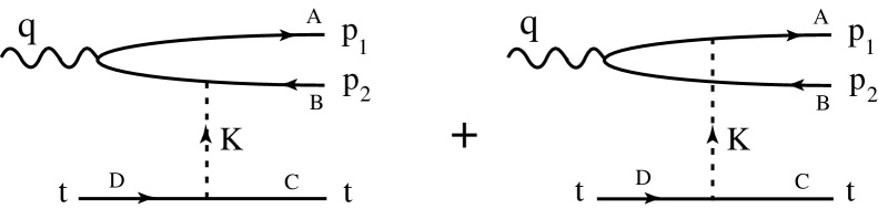
Figure 6: Amplitude for the process $\gamma g\to q\bar{q}$.

The standard infinite momentum frame expression for the $\gamma g\to q\bar{q}$ cross section in the limit where the photon energy $\nu\to\infty$ while the transverse momentum $p_{\perp}$ of the produced quarks and their squared invariant mass $\hat{s}=xs=2x\nu m_{N}$ are kept fixed is

$$\frac{d\sigma}{dp_{\perp}^{2}\,dz}=\frac{\pi e_{q}^{2}\alpha\alpha_{s}}{p_{\perp}^{4}}xG(x)\left[z^{2}+(1-z)^{2}\right]$$ (A.1)

where $p_{\perp}^{2}=z(1-z)\hat{s}$.

In the target rest frame (see Fig. 6) $z$ is the fraction of the photon longitudinal momentum carried by the quark,

$$\vec{p}_{1} = (\vec{p}_{1\perp},z\nu)$$

$$\vec{p}_{2} = (\vec{p}_{2\perp},(1-z)\nu+k^{z})$$ (A.2)

$$2\nu k^{z} = -\vec{p}_{1\perp}^{\ 2}/z-\vec{p}_{2\perp}^{\ 2}/(1-z)$$

The amplitude for photon scattering on a heavy quark $t$ in the limit we consider can then be written [22]

$$T(\gamma t\to q\bar{q}t) = ee_{q}g^{2}T_{AB}^{a}T_{CD}^{a}\frac{4m_{t}\nu z(1-z)}{k_{\perp}^{2}}$$ (A.3)

$$\times \left[\frac{\bar{u}(p_{1})\vec{\varepsilon}\cdot\vec{\gamma}v(p_{2}-k)}{p_{1\perp}^{2}}-\frac{\bar{u}(p_{1}-k)\vec{\varepsilon}\cdot\vec{\gamma}v(p_{2})}{p_{2\perp}^{2}}\right]$$

After summing and averaging over spins the square of the amplitude simplifies to

$$\overline{|T|^{2}}=16e_{q}^{2}\alpha\alpha_{s}^{2}(4\pi)^{3}\frac{N^{2}-1}{8N}\frac{4m_{t}^{2}\nu^{2}z(1-z)}{k_{\perp}^{2}p_{1\perp}^{2}p_{2\perp}^{2}}\left[z^{2}+(1-z)^{2}\right]$$ (A.4)

In the expression for the cross section

$$\frac{d\sigma}{dp_{1\perp}^{2}\,dz}=\frac{1}{4m_{t}^{2}(4\pi)^{4}}\int\frac{d^{2}\vec{k}_{\perp}}{z(1-z)\nu^{2}}\,\overline{|T|^{2}}$$ (A.5)

the $k_{\perp}$-dependence of the integrand is (for $k_{\perp}\ll p_{1\perp},\ p_{2\perp}$) of the form $1/k_{\perp}^{2}$. Here we introduce $R^{-1}\sim\Lambda_{QCD}$ as an infrared cut-off for the logarithmic integral, where $R$ is the nucleon radius, playing the role of a color screening length. To leading logarithmic accuracy the scattering occurs incoherently over the pointlike target quarks. The upper limit of the $k_{\perp}$-integration is set by $k_{\perp}\simeq p_{1\perp}$, where the approximation $\vec{p}_{2\perp}^{\ 2}=(\vec{k}_{\perp}-\vec{p}_{1\perp})^{2}\simeq\vec{p}_{1\perp}^{\ 2}$ fails and the integrand is more strongly damped in $k_{\perp}$. This defines the logarithmic approximation as

$$\log\left(\frac{p_{\perp}^{2}}{\Lambda_{QCD}^{2}}\right)\gg 1$$ (A.6)

In order to deal with measurable cross sections one has to average over the possible positions of the heavy target quark. We assume in this paper a uniform density for the target quark, denoted by $\rho$, and thus we multiply Eq. (A.5) by a factor $\rho V$ counting the number of static centres in one hard scattering, $V$ being the target volume.

Comparing the resulting expression for the $k_{\perp}$-integrated cross section with that of the infinite momentum frame result (A.1) we find

$$xG(x)=\rho V\,\frac{N^{2}-1}{2\pi N}\alpha_{s}(p_{\perp}^{2})\log\left(\frac{p_{\perp}^{2}}{\Lambda_{QCD}^{2}}\right)\ \>,$$ (A.7)

or, taking $N=3$,

$$\rho V=\frac{33-2n_{f}}{16}xG(x)$$ (A.8)

We have checked that the relation (A.8) is obtained also if one considers $\eta_{c}$ production through two-gluon fusion, by simply comparing the expressions for the cross section in the target rest frame obtained from Eq. (2.8) with that of the infinite momentum frame (see, eg, Ref. [25]).

References

- [1] J. H. Kühn, Phys. Lett. 89B (1980) 385; C. H. Chang, Nucl. Phys. B172 (1980) 425; E. L. Berger and D. Jones, Phys. Rev. D23 (1981) 1521; R. Baier and R. Rückl, Phys. Lett. 102B (1981) 364 and Z. Phys. C19 (1983) 251; J. G. Körner, J. Cleymans, M. Karoda and G. J. Gounaris, Nucl. Phys. B204 (1982) 6.
- [2] M. Krämer, J. Zunft, J. Steegborn and P. M. Zerwas, Phys. Lett. B348 (1995) 657; M. Krämer, Nucl. Phys. B459 (1996) 3.
- [3] A comprehensive review of the early fixed target data may be found in G. A. Schuler, CERN-TH.7170/94, hep-ph/9403387.
- [4] A. Sansoni, Talk at the 6th International Symposium on Heavy Flavour Physics, Pisa, 6-11 June 1995, Fermilab-Conf-95/263-E, Nuovo Cim. A109 (1996) 827.
- [5] M. L. Mangano, Talk at Xth Topical Workshop on Proton-Antiproton Collider Physics, Batavia, May 1995, Published in Batavia Collider Workshop 1995, p. 120, hep-ph/9507353.
- [6] M. Vänttinen, P. Hoyer, S. J. Brodsky and W.-K. Tang, Phys. Rev. D51 (1995) 3332.
- [7] R. Gavai, D. Kharzeev, H. Satz, G. A. Shuler, K. Sridhar and R. Vogt, Int. J. Mod. Phys. A10 (1995) 3043, hep-ph/9502270.
- [8] G. A. Schuler, CERN-TH/95-75, hep-ph/9504242.
- [9] J. A. Amundson, O. Éboli, E. Gregores and F. Halzen, Phys. Lett. B372 (1996) 127, hep-ph/9512248; and MADPH-96-942, hep-ph/9605295.
- [10] G. A. Schuler and R. Vogt, Phys. Lett. B387 (1996) 181, hep-ph/9606410.
- [11] M. Cacciari, M. Greco, M. L. Mangano and A. Petrelli, Phys. Lett. B356 (1995) 553, hep-ph/9505379.
- [12] E. Braaten and S. Fleming, Phys. Rev. Lett. 74 (1995) 3327, hep-ph/9411365; P. Cho and A. K. Leibovich, Phys. Rev. D53 (1996) 150, hep-ph/9505329 and Phys. Rev. D53 (1996) 6203, hep-ph/9511315.
- [13] E. Braaten, S. Fleming and T. C. Yuan, OHSTPY-HEP-T-96-001, hep-ph/9602374.
- [14] P. Hoyer, talk published in ‘Confinement Physics: Proc. 1st ELFE Summer School’, Eds. S.D. Bass and P.A.M. Guichon (Editions Frontieres, 1996), p.343, hep-ph/9511411.
- [15] E772 Collaboration, D. M. Alde et al., Phys. Rev. Lett. 64 (1990) 2479.
- [16] E772 Collaboration, D. M. Alde et al., Phys. Rev. Lett. 66 (1991) 133. See also M. J. Leitch et al., Nucl. Phys. A544 (1992) 197c.
- [17] D. M. Alde et al., Phys. Rev. Lett. 66 (1991) 2285. See also M. J. Leitch et al., Nucl. Phys. A544 (1992) 197c.
- [18] NA3 Collaboration, J. Badier et al., Z. Phys. C20 (1983) 101; S. Katsanevas et al., Phys. Rev. Lett. 60 (1988) 2121. See also: NA10 Collaboration, P. Bordalo et al., Phys. Lett. B193 (1987) 373.
- [19] J. Qiu and G. Sterman, ITP-SB-96-54, talk given at the Brookhaven Theory Workshop on Relativistic Heavy Ions, Upton, NY, 8-19 Jul 1996, hep-ph/9610476.
- [20] M. Gyulassy and X.-N. Wang, Nucl. Phys. B420 (1994) 583; R. Baier, Yu. L. Dokshitzer, A. H. Mueller, S. Peigné and D. Schiff, Nucl. Phys. B483 (1997) 291 and Nucl. Phys. B484 (1997) 265; B. G. Zakharov, LPTHE-Orsay 97-09, hep-ph/9704255.
- [21] J. C. Collins, D. E. Soper and G. Sterman, in “Perturbative Quantum Chromodynamics”, ed. A.H. Mueller, World Scientific, Singapore, 1990.
- [22] V. Del Duca, S. J. Brodsky and P. Hoyer, Phys. Rev. D46 (1992) 931; S. J. Brodsky, P. Hoyer and L. Magnea, Phys. Rev. D55 (1997) 5585, hep-ph/9611278.
- [23] A. Krzywicki, J. Engels, B. Petersson and U. Sukhatme, Phys. Lett. 85B (1979) 407; G. T. Bodwin and S. J. Brodsky, Phys. Rev. Lett. 47 (1981) 1799; P. Chiappetta and H. J. Pirner, Nucl. Phys. B291 (1987) 765; S. Gavin and M. Gyulassy, Phys. Lett. 214B (1988) 241; J. Hüfner, Y. Kurihara and H. J. Pirner, Phys. Lett. 215B (1988) 218; P. Jain and J. P. Ralston, hep-ph/9406394; J. Dolejší, J. Hüfner and B. Z. Kopeliovich, Phys. Lett. 312B (1993) 235; B. Z. Kopeliovich, hep-ph/9702365.
- [24] J. H. Kühn, J. Kaplan and E. G. O. Safiani, Nucl. Phys. B157 (1979) 125.
- [25] R. Baier and R. Rückl, Phys. Lett. 102B (1981) 364 and Z. Phys. C19 (1983) 251.