JET OBSERVABLES

IN THEORY AND REALITY

Davision E. Soper

Institute of Theoretical Science

University of Oregon

Eugene, Oregon 97403 USA

Abstract

I discuss the one jet inclusive jet cross section, $d\sigma/dE_{T}$ emphasizing the concept of infrared safety and the cone definition of jets. Then I estimate the size of power corrections to the jet cross section, which become important at smaller values of $E_{T}$.

Talk at the Rencontre de Moriond, QCD Session

Les Arcs, France, March 1997

Jet definitions and infrared safety

Jets are an obvious feature of the final state for $p+\bar{p}\to hadrons$. Although the jets are obvious, for a quantitative comparison of theory and experiment, one must carefully specify what one means by a jet. The jet definition associates with each jet a transverse energy $E_{T}$, a rapidity $\eta$, and an azimuthal angle $\phi$. Then one can form the inclusive jet cross section

$${d\sigma\over dE_{T}}={1\over\eta_{2}-\eta_{1}}\int_{\eta_{1}}^{\eta_{2}}\!\!d\eta\int_{0}^{2\pi}\!\!d\phi\ {d\sigma\over dE_{T}d\eta d\phi}.$$ (1)

With a suitable definition the cross section has the form

$${d\sigma\over dE_{T}\,d\eta\,d\phi}\approx\ \sum_{a,b}\int_{x_{A}}^{1}\!d\xi_{A}\int_{x_{B}}^{1}\!d\xi_{B}\ {f_{a/A}(\xi_{A},\mu)}\ {f_{b/B}(\xi_{B},\mu)}\ {{{d\hat{\sigma}^{ab}(\mu)\over dE_{T}\,d\eta\,d\phi}}},$$ (2)

where the $f_{a/A}(\xi,\mu)$ are the parton distributions and where ${{{d\hat{\sigma}^{ab}/[dE_{T}\,d\eta\,d\phi]}}}$ is the perturbatively calculated hard scattering function. (The lowest order is $\alpha_{s}^{2}$; current calculations^?,?) reach $\alpha_{s}^{3}$.)

The cross section should be insensitive to long times $\Delta t\gg 1/E_{T}$. However, we know that, long after the hard interaction, soft particles are emitted or absorbed. Thus, $d\sigma/dE_{T}$ should be insensitive to soft particles. We know also that long after the hard interaction a fast particle can split into two collinear particles or two collinear fast particles can join. Thus $d\sigma/dE_{T}$ should be insensitive to collinear splitting and joining. A measureable quantity such as a jet cross section that has these properties is said to be infrared safe.

I consider here the “Snowmass Accord” jet definition^?). Define a jet cone of radius R in $\eta$-$\phi$ space. Typically, $R=0.7$. The jet variables $E_{T,J},\eta_{J},\phi_{J}$ are defined in terms of the particles by

$$E_{T,J}=\sum_{i\in{\rm cone}}E_{T,i}\,,$$ (3)

$$\phi_{J}={1\over E_{T,J}}\sum_{i\in{\rm cone}}E_{T,i}\ \phi_{i}\,,\hskip 28.45274pt\eta_{J}={1\over E_{T,J}}\sum_{i\in{\rm cone}}E_{T,i}\ \eta_{i}\,.$$ (4)

The cone axis must agree with the jet axis $(\eta_{J},\phi_{J})$. One iterates until agreement is reached.

There are some difficulties that require one to amend this jet definition.^?,?) First, sometimes the cones overlap. If there is more than some specified amount of transverse energy in the overlap region, then one merges the jets. Otherwise, one splits the transverse energy in the overlap region between the two jets. Second, there will be transverse energy in the jet cone that is not related to the high $P_{T}$ parton that made the jet but instead is associated with the underlying event. Accordingly, one subtracts $\rho\,\pi R^{2}$ from $E_{T}$, where $\rho$ is the average $E_{T}$ per unit $d\eta\,d\phi$ in minimum bias events. At the Fermilab Tevatron, $\rho\,\pi(0.7)^{2}\approx 1.1{\ \rm GeV}$. Note that one does not do this in the corresponding order $\alpha_{s}^{3}$ theoretical calculation since the underlying event is not part of the calculation.

In the theoretical calculation, one often modifies^?) the Snowmass defintion to restrict merging partons into jets according to a variable $R_{\rm sep}$. If two partons have

$$(\eta_{1}-\eta_{2})^{2}+(\phi_{1}-\phi_{2})^{2}>R_{\rm sep}^{2}\,,$$ (5)

one does not merge them, even though

$$(\eta_{i}-\eta_{\rm jet})^{2}+(\phi_{i}-\phi_{\rm jet})^{2}<R^{2},\hskip 28.45274pti=1,2.$$ (6)

Why? Studies^?) of the $E_{T}$ distribution within jets suggest that the experimental jet algorithms fail to merge subjets that are rather far separated. The value $R_{\rm sep}=1.3R$ is suggested. This lowers the theoretical cross section about 4%.

The theory for jet production comes with theoretical uncertainties. There are uncalcuated $\alpha_{s}^{4}$ and higher perturbative contributions. A typical estimate^?) of this uncertainly is $\pm 15\%$. In addition, there is uncertainty in the parton distributions. One may guess $\pm 20\%$ for this uncertainty for $E_{T}<300{\ \rm GeV}$. The uncertainty is presumably larger for $E_{T}>300{\ \rm GeV}$  because the gluon distribution is largely unknown^?) at large $x$. Finally, there are corrections suppressed by a power of “1 GeV”/$E_{T}$. In the remainder of this talk, I attempt to estimate these corrections using simple models.

Power suppressed corrections

In this section, I address power suppressed corrections to the theory. I will present graphs of (Data - Theory ) /Theory. Both data and theory refer to the jet cross section $d\sigma/dE_{T}$ for $0.1<|\eta|<0.7$ and $R=0.7$ as in Eq. (1). The data is from CDF^?) and has been corrected by CDF by subtracting from the jet $E_{T}$ an estimate of the transverse energy contained in the jet cone that arises from the underlying event ($\Delta E_{T}\approx$ 1.1 GeV). The theory here is straightforward order $\alpha_{s}^{3}$ QCD with CTEQ4M partons. The theoretical calculation uses an $R_{\rm sep}$ correction to the Snowmass algorithm, with $R_{\rm sep}=1.3R$.

Splash in. In $\alpha_{s}^{3}$ theory, the transverse energy of a jet comes from one or two partons. It is the decay products of these partons (using the picture embedded in Monte Carlo models), that one wants to capture in the jet cone. However, other particles can splash into the cone. The underlying event creates soft particles that will get into the cone. An estimate of this effect has already been subtracted from $E_{T}$ in the data, so we do not consider it further. In addition, the accelerated initial state partons radiate soft gluons, whose decay products can splash into the cone. Let us try to estimate this effect.

If transverse energy $\Delta E_{T}^{\rm in}$ is added to the jet $E_{T}$, the cross section should change by

$${d\sigma\over dE_{T}}\approx\left(d\sigma\over dE_{T}\right)_{\!\rm NLO}\left\{1+n\ {\Delta E_{T}^{\rm in}\over E_{T}}\right\},$$ (7)

where

$$n(\ln(E_{T}))=-{d\over d\ln(E_{T})}\,\ln\left[\left(d\sigma\over dE_{T}\right)_{\!\rm NLO}\right].$$ (8)

The factor $1/E_{T}$ makes this a small correcton for large $E_{T}$. However, $n$ is large.

Marchesini and Webber^?) have suggested a method for estimating from data the level of transverse energy in jet events without including the $E_{T}$ from the third of three partons in a perturbative calculation. Lacking such a data-based analysis, I use Marchesini and Webber’s Monte Carlo study for the amont of extra splash-in:

$$\Delta E_{T}^{\rm in}\approx 0.6{\ \rm GeV}.$$ (9)

Splash-out. Some of the partonic transverse energy can leak out of the jet cone. The order $\alpha_{s}^{3}$ perturbation theory gets this effect partly right: in a three parton final state the third parton can escape the jet cone. However, using the picture embedded in Monte Carlo models, the late stages of partonic branching and the final hadronization of the partons can also result in transverse energy escaping the jet cone. Here is a simple model for this effect.

Consider the hadrons that represent the decay products of a high $E_{T}$ parton. Let $\eta$ be the rapidity of the hadrons relative to jet axis. Let $\vec{k}_{T}$ be the transverse momentum of the particles relative to jet axis. Let the distribution of hadrons be

$${dN\over d\eta d\vec{k}_{T}}={A\over\pi\langle k_{T}^{2}\rangle}\ \exp\left\{-k_{T}^{2}/\langle k_{T}^{2}\rangle\right\},$$ (10)

where $A$ is the number of hadrons per unit rapidity and $\langle k_{T}^{2}\rangle$ is average $k_{T}^{2}$ of the hadrons. Then the $E_{T}$ lost is approximately

$$E_{T}^{\rm out}=\int_{0}^{\eta_{1}}\!\!d\eta\int\!d\vec{k}_{T}\ {1\over 2}|\vec{k}_{T}|e^{\eta}\ {dN\over d\eta d\vec{k}_{T}},$$ (11)

where $\eta_{1}=-\ln\left(\tan(R/2)\right).$ Performing the integral gives

$$E_{T}^{\rm out}={\sqrt{\pi}\over 4}A\sqrt{\langle k_{T}^{2}\rangle}\left(e^{\eta_{1}}-1\right).$$ (12)

Taking $\sqrt{\langle k_{T}^{2}\rangle}$ = 0.3 GeV and^?) $A$ = 5, I find

$$E_{T}^{\rm out}\approx 1.1{\ \rm GeV}.$$ (13)

This estimate can be used to correct the theoretical cross section, using the analog of Eq. (7) (with the opposite sign for $E_{T}^{\rm out}$ instead of $E_{T}^{\rm in}$).

In Fig. 1 below, I show the data compared to theory. In the same graph, I show a curve representing (Modified Theory $-$ Theory) / Theory, where the modified theory includes a correction for splash-in/splash-out. Evidently, the correction does not improve the agreement between theory and experiment. The size of the correction provides some estimate of the theory error from this source.

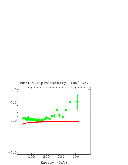
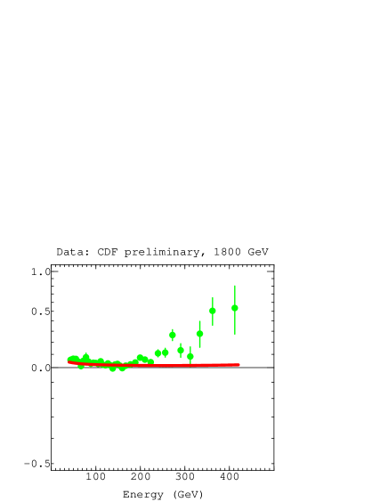
Figure 1: $(Data-Theory)/Theory$ for the jet cross section versus transverse energy $E_{T}$. In the left hand graph, the curve shows the correction to the theory for splash-in/splash-out. In the right hand graph, the curve shows the correction to the theory for $k_{T}$ smearing.

Transverse momentum smearing. In an order $\alpha_{s}^{3}$ calculation, incoming partons have zero transverse momentum. Thus the observed jet can recoil against only one or two jets. But in a more realistic model, the incoming partons can radiate multiple soft gluons, each carrying some transverse momentum. In addition, the partons in the proton wave function can have a “primordial $k_{T}$” by virtue of being bound in a hadron of finite size.

Let us try a simple model that accounts for these effects. There is a risk of double counting, since we may count the same gluon both as one of the multiple soft gluons and as one of the final state gluons in the hard scattering. We simply hope that the double counting effect will be small.

Define a function $G(\vec{P}_{T})$ that represents the measured cross section for one jet inclusive production:

$$G(\vec{P}_{T})={d\sigma\over d\vec{P}_{T}}={1\over 2\pi P_{T}}\ {d\sigma\over dP_{T}},\hskip 28.45274ptP_{T}\equiv E_{T}.$$ (14)

Let $G\!\left(\vec{P}_{T}\right)_{\rm NLO}$ be the same cross section calculated at next to leading order. Then we can make a simple model for $G(\vec{P}_{T})$:

$$G(\vec{P}_{T})=\int\!d\vec{k}_{T}\ \rho(\vec{k}_{T};P_{T})\ G\!\left(\vec{P}_{T}-{1\over 2}\,\vec{k}_{T}\right)_{\rm NLO},$$ (15)

where $\rho(\vec{k}_{T};P_{T})$ is a smearing function that represents the probability that the partons entering the hard scattering had transverse momentum $\vec{k}_{T}$. This function depends on $P_{T}$ because large $P_{T}$ in the hard scattering means more soft gluon radiation.

Supposing that $k_{T}\ll P_{T}$, we have

$$G(\vec{P}_{T}) \approx \int\!d\vec{k}_{T}\ \rho(\vec{k}_{T};P_{T})\ \biggl{\{}G(\vec{P}_{T})_{\rm NLO}$$ (16)

$$-{1\over 2}k_{T}^{i}\nabla_{i}G(\vec{P}_{T})_{\rm NLO}+{1\over 8}k_{T}^{i}k_{T}^{j}\nabla_{i}\nabla_{j}G(\vec{P}_{T})_{\rm NLO}\biggr{\}}.$$

Define

$$n(\ln(P_{T}))=-{d\over d\ln(P_{T})}\,\ln\left(2\pi P_{T}\ G(\vec{P}_{T})_{\rm NLO}\right).$$ (17)

Then

$${d\sigma\over dE_{T}}\approx\left(d\sigma\over dE_{T}\right)_{\!\rm NLO}\left\{1+{(n+1)^{2}-n^{\prime}\over 16}\ {\langle k_{T}^{2}\rangle\over E_{T}^{2}}\right\}.$$ (18)

To obtain a quantitative estimate, I use $n(\ln(E_{T}))$ from a NLO calculation and

$$\langle k_{T}^{2}\rangle\approx 2mE_{T},\hskip 28.45274ptm=0.35{\ \rm GeV}.$$ (19)

This formula is a rule of thumb. The number for $m$ is based on identifying $2E_{T}$ with $M_{Z}$ in $p+\bar{p}\to Z+X$, supposing that the $k_{T}$ distribution of the $Z$ is approximately gaussian for $k_{T}\ll M_{Z}$, and identifying $\langle k_{T}^{2}\rangle$ by noting that^?) $d\sigma/dk_{T}$ peaks at $k_{T}\approx 4{\ \rm GeV}$. Then

$${d\sigma\over dE_{T}}=\left(d\sigma\over dE_{T}\right)_{\!\rm NLO}\left\{1+{(n+1)^{2}-n^{\prime}\over 8}\ {m\over E_{T}}\right\}.$$ (20)

(There is computer code by Baer and Reno^?) that does this sort of smearing for direct photon production, using a Monte Carlo style calculation.) In Fig. 1, I show the data compared to NLO theory with a correction for $k_{T}$ smearing shown as a curve.

The net result. In Fig. 2, I show the data compared to the NLO theory with the net correction for splash-in/splash-out and $k_{T}$ smearing shown as a curve.

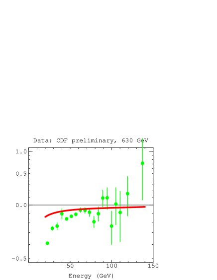
Figure 2: Graph of $(Data-Theory)/Theory$ versus $E_{T}$ for with curves showing the net power supressed correction as estimated using Eqs. (7) and (20). The left hand graph is for $\sqrt{s}=1800{\ \rm GeV}$ while the right hand graph is for $\sqrt{s}=630{\ \rm GeV}$

The net correction is quite small. If we take the size of the various corrections as an error estimate, we can estimate a theory error from power suppressed corrections of about $\pm 10\%$ at $E_{T}=40{\ \rm GeV}$ and $\pm 4\%$ at $E_{T}=200{\ \rm GeV}$.

In Fig. 2, I also show the CDF data^?) at $\sqrt{s}=630{\ \rm GeV}$ compared to the NLO theory with the net correction for splash-in/splash-out and $k_{T}$ smearing shown as a curve. I use the same parameters as for $\sqrt{s}=1800{\ \rm GeV}$ except that (estimating from the Monte Carlo study used earlier^?)), I reduce the splash-in parameter $E_{T}^{\rm in}$ from 0.6 GeV to 0.3 GeV.

If we take the size of the various corrections as an error estimate, then the estimated error is larger than at $\sqrt{s}=1800{\ \rm GeV}$, perhaps $\pm 20\%$ at $E_{T}=20{\ \rm GeV}$. It may be significant that, while the net effect at $\sqrt{s}=1800{\ \rm GeV}$ is really quite small, the net effect at $\sqrt{s}=630{\ \rm GeV}$ is not so small, and is in the right direction to improve the agreement between theory and experiment.

I thank Anwar Bhatti of the CDF Collaboration for help with the CDF data.

References

- [1] S. D. Ellis, D. E. Soper and Z. Kunszt, Phys. Rev. Lett. 64, 2121 (1990).
- [2] W. T. Giele, E. W. N. Glover and D. A. Kosower, Phys. Rev. Lett. 73, 2019 (1994).
- [3] J. S. Huth et al., in Research Directions for the Decade, Proceedings of the Summer Study on High Energy Physics, Snowmass, CO, June 1990, edited by E. L. Berger (World Scientific, Singapore, 1992).
- [4] F. Abe et al. (CDF Collaboration), Phys. Rev. D 45, 1448 (1992).
- [5] S. Abachi et al. (D0 Collaboration), Phys. Lett. B 357, 500 (1995).
- [6] S. D. Ellis, D. E. Soper and Z. Kunszt, Phys. Rev. Lett. 69, 3615 (1992).
- [7] J. Huston, E. Kovacs, S. Kuhlmann, H. L. Lai, J. F. Owens, D. E. Soper and W.-K. Tung, Phys. Rev. Lett. 77, 444 (1996).
- [8] F. Abe et al. (CDF Collaboration), Phys. Rev. Lett. 77, 438 (1996); P. Melese (CDF Collaboration), talk at Les Rencontres De Physique De La Vallee D’Aoste, La Thuille, Italy, March 1997.
- [9] G. Marchesini and B. R. Webber, Phys. Rev. D 38, 3419 (1988).
- [10] Jing-Chen Zhou, University of Oregon Ph.D. Thesis, 1997.
- [11] D. L. Puseljic (D0 Collaboration), talk at Workshop, Fermilab, May 1995. See R. K. Ellis, W. J. Stirling and B. R. Webber, QCD and Collider Physics (Cambridge, Cambridge, 1996), p. 326.
- [12] H. Baer and M. H. Reno, Phys. Rev. D 54, 2017 (1996).
- [13] P. Melese (CDF Collaboration), talk at Les Rencontres de Physique de la Vallée d’Aoste, La Thuille, Italy, March 1997.