Photoproduction

Abstract

Some selected topics in photoproduction are reviewed. In particular, the focus is on quasi-real photon–proton scattering as measured at HERA. Single & dijet rates and jet profiles are discussed, as are open charm production and inelastic charmonium production. The many intriguing theoretical issues which can be addressed through study of these processes are highlighted.

Introduction

In this talk, I’m going to present a summary of recent developments in photoproduction at HERA. By “photoproduction” I mean $\gamma p$ interactions in which the photon is close to being on its mass shell. Furthermore, I shall focus on processes in which there exists at least one hard scale – so that we have the chance to use perturbation theory. I’m going to divide the talk into 4 parts: jets (single & dijet rates); jet profiles; open charm production ($D^{*}$’s); inelastic charmonium production. I won’t talk about processes with rapidity gaps, since these diffractive processes are covered in other people’s presentations.

I Jet cross-sections

I wish to start by recalling some basic terminology. It is convenient to talk about two classes of photoproduction event: those in which all of the energy of the incoming photon is delivered to the hard subprocess (these are called “direct” processes) and those in which only part of the incoming photon energy goes into producing the hard subprocess (these are called “resolved” processes).

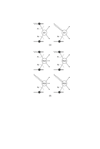
Figure 1: LO (a) and NLO (b) direct and resolved contributions to jet photoproduction

Fig.1(a) shows the lowest order contribution from these two types of process in the case of jet production. The dotted lines show where we chose to separate the hard process from the non-perturbative parton distribution functions. The factorization scales $\mu_{\gamma}$ and $\mu_{p}$ are in principle arbitrary but a good choice would be to pick them to be $\sim p_{T}$ (i.e. the jet transverse momentum) since this choice will account for the fact that the incoming partons have a large region of transverse phase space into which they can radiate other partons. Nonetheless, it is certainly true that the theoretical calculation will exhibit a strong sensitivity to any variation in the factorization scales since the $2\to 2$ hard subprocesses contain no dependence upon the factorization scales whereas the parton distribution functions do. For example, we could effectively turn off all parton evolution by picking the factorization scales to be much smaller than $p_{T}$. At this level of calculation, it is clear what we mean by “direct” and “resolved” processes.

In Fig.1(b), the ${\cal O}(\alpha_{s})$ corrections to the jet production process are shown. We have to account for the fact that the hard subprocess can radiate off 3 partons into the final state as well as the virtual corrections to the 2 parton final state. Again, we can classify diagrams as being direct or resolved. However, there are collinear divergences associated with the 3 parton final state. This means that the 3 parton hard subprocesses are dependent upon the factorization scales. Let us focus on the $\mu_{\gamma}$ dependence. By varying $\mu_{\gamma}$ we vary the amount of the next-to-leading order (NLO) $2\to 3$ processes that should really be attributed to the lowest order (LO) resolved process. In particular, the amount of NLO direct that should rightfully be factorized into the LO resolved contribution depends upon the choice of $\mu_{\gamma}$. In this way, the strong dependence upon the factorization scales is reduced by including the NLO contribution. Also, we can no longer uniquely define the separation of direct and resolved processes.

I.1 Single jet inclusive

Figure 2: Inclusive single jet cross-section integrated above $E_{T}=8$ GeV (a), 11 GeV (b) and 17 GeV (c). The data 1jetZeus are compared with the NLO calculation of KKS . Dotted line shows the direct contribution, dashed line the resolved and solid the total.

NLO calculations of the single jet inclusive rate have been available for a while now jets . Comparison with the data 1jetH1 ; mievi ; 1jetZeus should tell us about the parton content of the photon, and in particular its gluonic content (which is not really constrained from elsewhere). However, in just the region where one expects sensitivity to the gluon in the photon the NLO theory is not working! Forward jets (i.e. those heading largely in the proton direction and hence having positive pseudo-rapidity, $\eta$) with modest values of transverse energy, $E_{T}$, are most sensitive to the gluon content of the photon. Fig.2 compares the 1993 ZEUS data with the theoretical calculations of Klasen, Kramer & Salesch KKS which use the GS(HO) photon parton densities GSpdf and the MRSD- proton densities MRS . Comparison reveals that the theory is well below the data for forward jets at the lower $E_{T}$ values (this conclusion is also supported by the H1 data and the ZEUS 1994 data). The problem seems not so bad as $E_{T}$ is increased. One might argue that the difference between theory and data should be attributed to the fact that the photon parton density functions need adjusting, i.e. more gluons are required at low $x$. However, one should be cautious. These forward jets are also much broader than expected from Monte Carlo studies.

It is possible that the broadening of the forward jets comes about in the presence of a large underlying event. Models which attempt to account for some or all of this physics mis ; BFS have received some support from the data mievi . In particular, simple models of multiple parton scattering produce large effects in the forward region, e.g. see BFS . Multiple parton scattering is anticipated on the grounds that forward jets at low $E_{T}$ are produced as a result of interactions between slow partons in the colliding particles. We know that QCD predicts a proliferation of these slow partons, and as such it may well be that more than one pair of them can interact in each $\gamma p$ interaction.

In summary, the HERA experiments are providing precise data which is ready for comparison with the theory. However, before we can safely extract the photon parton distribution functions we really need to understand what is going on with the forward jets. I think the issue of the forward jets is potentially very interesting. If multiple interactions really are present, then we are looking at a new regime of QCD.

I.2 Dijets

Data on two or more jets 2jetZeus ; angle ; 2jetH1 provides us with further options to test QCD and understand the nature of the “strongly interacting” photon. In particular, the two highest $E_{T}$ jets can be used to compute the variable

$$x_{\gamma}=\frac{\sum_{{\rm jets}}E_{T}e^{-\eta}}{2yE_{e}}.$$ (1)

At lowest order, $x_{\gamma}=1$ for direct events and $x_{\gamma}<1$ for resolved events. A cut on $x_{\gamma}$ therefore provides a physical definition of direct and resolved event classes. ZEUS has defined direct enriched and resolved enriched samples by separating events according to a cut at $x_{\gamma}=0.75$. The direct enriched sample is very sensitive to the small-$x$ gluon content of the proton: the more backward the dijets, the lower the $x$ values in the proton that are probed. Conversely, the resolved enriched sample is sensitive to the gluon content in the photon. In addition, NLO calculations for the dijet rates are now available for comparison with the data KK ; O . Let’s summarize the situation as it stands right now.

Figure 3: Inclusive dijet cross-section for direct and resolved enriched processes as a function of the average jet rapidity, $\bar{\eta}$, and integrated over the rapidity difference, $\Delta\eta$, of the two highest $E_{T}$ jets, i.e. $|\Delta\eta|<0.5$, and $E_{T}$ as shown. The LO and NLO theory of KK is compared to the data 2jetZeus . The GRV GRV and CTEQ3M CTEQ NLO ${\overline{MS}}$ parton densities were used.

For $x_{\gamma}>0.75$, as can be seen from Fig.3, the NLO theory does a good job. However (and this is not shown in the plot) there remains quite a large contamination from the large-$x$ part of the photon quark distribution functions. This arises because of the harder form of the photon quark densities. To unravel the effects of the low-$x$ gluons in the proton from the large-$x$ quarks in the photon requires a tighter cut on $x_{\gamma}$. This is feasible, for example for $E_{T}>30$ GeV and 250pb^-1 of $ep$ data one expects around 4500 events with $x_{\gamma}>0.9$ HERAwkp . Also, comparison between data and theory requires that the same jet algorithm is used. To facilitate a clean comparison between data and theory, the ZEUS collaboration has started to used the $k_{t}$-cluster algorithm ktclus .

For $x_{\gamma}<0.75$ Fig.3 reveals that the theory falls well below the data for the lowest $E_{T}$ forward dijets. The effect exhibits a strong dependence upon the $E_{T}$ cut, which suggests that it cannot be explained by modifying the parton distribution functions of the photon in any sensible way. Presumably, this is the same problem as that which we encounter for the single jets. Again, multiple interactions help fix the problem.

The dijet measurements shown in Fig.3 have been made with a cut on the minimum $E_{T}$ of the jets and the cut is the same for both jets. This introduces a further theoretical problem. This arises because most of the jets will be produced around the minimum allowable $E_{T}$, i.e. the typical difference between the jet transverse momenta, $\Delta p_{T}$, will be small. So, the 3 parton final state (which is present in the NLO calculation) must have one of the partons either collinear with another, or very soft. The collinear configuration is easy to deal with (it is factorized) but the soft parton emission leads to a $\ln\Delta p_{T}$ contribution. This large logarithm signals that multiple soft parton emission is important. These soft parton effects can be studied by looking explicitly at the $\Delta p_{T}$ distribution of the dijets or they can be avoided by making a cut which keeps away from $\Delta p_{T}\approx 0$.

Figure 4: Dijet angular distribution

Complementary to the jet rapidity and $E_{T}$ distributions is the distribution in the polar angle of the jets, as defined in the dijet centre-of-mass frame. Such a measurement is insensitive to the parton density functions but sensitive to the subprocess which drives the jet production. Fig.4 shows the data angle and the good agreement with NLO theory O . The steepening of the $\cos\Theta^{*}$ distribution as $|\cos\Theta^{*}|\to 1$ is greater in the resolved enriched sample than in the direct enriched sample due simply to the fact that the resolved process proceeds predominantly through $t$-channel gluon exchange whilst the direct processes go via $t$-channel quark exchange.

In conclusion, the dijets provide information which complements the single jet measurements. The data is now reaching a high level of precision, and comparison with NLO theory has revealed a number of pressing issues. In particular, we need to understand better the forward jets, ensure that we are using the most convenient jet algorithm, and be aware of any sensitivity from soft parton emission. Once these issues have been addressed, we can expect to gain further insight into the gluon content of both the photon and proton.

II Jet Shapes

Now I want to address the question: “What is a jet?”. An observable which has been used to investigate this question is the shape variable $\psi(r,R,E_{T},\eta)$ which is the fraction of the jet (of cone size $R$) energy lying within a cone of size $r$ EKS . The lowest non-trivial order for this quantity involves the 3 parton matrix elements. To compute to order $\alpha_{s}^{2}$ requires the 4 parton final state matrix elements GK . Klasen & Kramer have been able to fit the ZEUS data on jet shapes jetshapes but only after introducing the parameter, $R_{{\rm sep}}$, into their calculations KlK . Let’s take a closer look at the $R_{{\rm sep}}$ parameter.

It’s a good idea to first remind ourselves of the steps involved in building jets using a cone algorithm cone . The ZEUS jets are found using an iterative cone algorithm (PUCELL). This algorithm defines some threshold energy, $E_{0}$, and calorimeter cells above this energy define the seeds for the jet finding. A jet is formed by summing all cells within a distance $R$ (in $\eta-\phi$ space) of the seed cell. If, after this, the jet axis no longer coincides with that of the original seed cell then the new jet axis is used and all cells within $R$ of it are used to redefine the jet. This process is iterated until a stable jet direction is achieved. It is possible that some of the jets overlap and so some criterion needs to be established to decide what should be done with these jets. For example, if one of the overlapping jets has more than 75% of its energy in common with another jet then one could merge the two jets, whilst if the overlap energy is less then one could split the two jets by assigning particles to the jet to which they are nearest. Finally, jets are accepted if their $E_{T}$ is larger than some minimum value. In the theoretical case, two partons are combined if they lie within a distance $R_{ij}$ of each other, where

$$R_{ij}\leq{\rm min}\left[\frac{(E_{Ti}+E_{Tj})R}{{\rm max}(E_{Ti},E_{Tj})},R_{{\rm sep}}\right].$$ (2)

We have introduced $R_{{\rm sep}}$ into this definition, it is introduced so as to simulate the effect of seed finding. For example, two partons with equal $E_{T}$’s lying a distance $2R$ apart could be considered to form a single jet (the partons lying on the edge of the jet cone). Such a configuration could not occur in the experimental algorithm, since there is no seed cell in between the two partons. As a result, for a 3 (or less) parton final state, picking $R_{{\rm sep}}=R$ should match the theoretical and experimental definition of the jets. Notice that the 3 parton final state does not call for any jet merging. By fitting $R_{{\rm sep}}$ to the data, one is accounting for higher order effects by fitting a single parameter (to fit the data Klasen & Kramer need to vary $R_{{\rm sep}}$ from 1.3 to 1.8 for jets with $\eta\approx-1$ to $\eta\approx 2$ respectively). For example, parton shower and hadronization effects (plus, maybe, multiple parton scattering) all effect the final state and we do not really learn much about them by tuning the theoretical calculation. Fig.5 demonstrates that forward jets are broader, as I claimed earlier. It also shows how multiple parton interactions can help improve the situation. It really is a challenge to theorists to explain the variation of $R_{{\rm sep}}$.

Figure 5: Jet shape from single jet production. Comparison between data jetshapes and PYTHIA, both with and without multiple parton scattering (MI), is shown.

Steps in this direction require a truly NLO calculation of the jet shape variable. As mentioned above, this means we need to consider the 4 parton final state. At this point, we realise that the iterative cone algorithm is not infra-red safe. By this we mean that it is not insensitive to the addition of a soft parton GK . To see this consider the 4 parton final state illustrated in Fig.6. The middle of the upper 3 arrows denotes a soft parton, which has energy just above the threshold energy, $E_{0}$. The presence of this seed in between the two hard partons would cause all 3 partons to be merged into a single jet. So our shape variable is sensitive to the cell threshold energy. This is an acute problem at any fixed order in perturbation theory (beyond LO). However, a strong $E_{0}$ dependence isn’t seen in Monte Carlo studies. Let me outline the basic idea as to why this should be so GK ; MikeS . Denote the probability for emitting a single parton into the overlap region, $P_{1}$, where

Figure 6: A four parton final state

$$P_{1}\sim\alpha_{s}\ln\frac{E_{T}}{E_{0}}.$$ (3)

This probability exponentiates on summing over all possible numbers of soft partons, i.e.

$$P_{{\rm all}}\sim 1-{\rm e}^{-P_{1}}.$$ (4)

So as $E_{0}\to 0$ a soft parton is guaranteed to be in the overlap region, i.e. $P_{{\rm all}}\to 1$. Thus we see that, on expanding the exponential, any finite order in $\alpha_{s}$ is sensitive to large $\ln E_{0}$ terms but that this sensitivity goes away on summing to all orders (as is done in the parton shower routines). As pointed out by Steve Ellis SE this problem can be fixed simply be redefining the jet algorithm, so that the mid-point between jets is always treated as a seed, regardless of any activity. Alternatively, the $k_{t}$ cluster algorithm avoids such problems. I think it is fair to say that studies on jet structure are reaching the point where theory really is starting to address the important issues. We should learn much over the coming few years.

III Open Charm

The photoproduction of charm quarks at large $p_{T}$ is a process which involves two large scales, $p_{T},m_{c}\gg\Lambda$ and as such, makes life more complicated from the theoretical point of view. Good data, which can be expected in the future (especially if the charm can be tagged using a microvertex detector), will surely shed light on this intriguing area. At present, there are two main routes used in theoretical calculations. I’ll start by describing briefly each.

Massive Charm: The charm quark mass is considered to provide the hard scale, as such charm only ever appears in the hard subprocess and there is no notion of radiatively generated charm in the sense of parton evolution massive . This means that terms $\sim\alpha_{s}\ln(p_{T}^{2}/m_{c}^{2})$ are not summed to all orders (in the parton distribution and fragmentation functions). As such, we might expect this approach to become less accurate when $p_{T}^{2}\gg m_{c}^{2}$. However, it does provide a systematic way of accounting for charm quark mass effects, which will be important for $m_{c}\sim p_{T}$.

Massless charm: In this approach, the charm quark is treated as massless (above threshold), and as such is treated like any other light quark in the parton evolution equations and hard subprocess cross-sections. The $\ln(p_{T}/m_{c})$ terms are now summed to all orders, but charm quark mass effects are ignored. So, this approach should get better as $p_{T}/m_{c}$ increases.

At present the data cdatH1 ; cdatZeus ; low lies in the intermediate region where $p_{T}<10$ GeV, i.e. it is not clear which, if any, of the two approaches should be used. In order to compute the inclusive $D^{*}$ rate, one needs the appropriate fragmentation function. Either the Peterson Peterson form or the $x^{a}(1-x)^{b}$ form do a good job, and have been well constrained by $e^{+}e^{-}$ data.

Figure 7: Comparison of the $D^{*}$ cross-section data cdatH1 with the calculation of CG .

Initial comparison between theory and data suggested that the massive charm calculation was too low, e.g see low . More recently, the situation has changed somewhat CG ; BKKS . The full NLO calculations require that the fragmentation function be consistently extracted from the $e^{+}e^{-}$ data. When this is done, Cacciari and Greco find that the theoretical predictions are increased significantly relative to what is found using the softer (LO) fragmentation functions CG . This is true for both massless and massive charm calculations and, within theoretical uncertainties, both are now consistent with the present data. For example, Fig.7 is a plot from CG , which shows that the NLO theory assuming massless charm agrees well with the data.

More data at large $p_{T}$ and increased statistics at intermediate $p_{T}$ will certainly help in our study of the interplay of $\ln(p_{T}^{2}/m_{c}^{2})$ and $m_{c}^{2}/p_{T}^{2}$ effects. In addition, for $p_{T}\gg m_{c}$ we have the possibility to study the “intrinsic” charm within the photon (charm in dijets offers good prospects here).

IV Charmonium

Originally, inelastic photoproduction of charmonium, e.g. $J/\psi$, was advertised as an ideal way to extract the gluon density in the proton (since it is driven by photon-gluon fusion into a $Q\bar{Q}$ pair). More recently, NLO calculations have put a dampener on this goal (as we shall see shortly). However, there has been a great deal of recent interest in the non-relativistic QCD (NRQCD) approach to heavy quarkonium production, and the inelastic photoproduction of heavy quarkonia provides the ideal opportunity to test NRQCD.

Figure 8: Leading contribution to quarkonium photoproduction.

Bodwin, Braaten and Lepage derived a factorization formula which describes the inclusive production (and decay) of a heavy quarkonium state BBL . In the case of photoproduction, Fig.8 shows the lowest order contribution. The NRQCD factorization formula for the corresponding cross-section reads

$$d\sigma(H+X)=\sum_{n}d\hat{\sigma}(Q\bar{Q}[n]+X)\langle O^{H}_{n}\rangle.$$ (5)

$X$ denotes that the process is inclusive, $d\hat{\sigma}(Q\bar{Q}[n]+X)$ is the perturbatively calculable cross-section for $\gamma p\to Q\bar{Q}+X$ and it can be written as a series expansion in $\alpha_{s}(m_{Q})$. The $Q\bar{Q}$ pair is produced with quantum numbers $n$. The matrix element, $\langle O^{H}_{n}\rangle$, contains the long distance physics associated with the formation of the quarkonium state $H$ from the $Q\bar{Q}$ state – it is essentially the probability that the pointlike $Q\bar{Q}$ pair forms $H$ inclusively. The typical scale associated with this part of the process is $\sim m_{Q}v$ which is much smaller than $m_{Q}$ ($v$ is the relative velocity of the $Q\bar{Q}$ pair, and is small for heavy enough quarks). This hierarchy of scales underlies the NRQCD factorization. Note that the $Q\bar{Q}$ state is not restricted to having the same quantum numbers as the meson. Fortunately, there exist “velocity scaling rules” which allow us to identify which states, $n$, are the most important. More precisely, the “velocity scaling rules” order the operators $\langle O^{H}_{n}\rangle$ according to how many powers of $v$ they contain, i.e. relativistic corrections can be computed systematically.

The NRQCD approach therefore provides us with a systematic way of computing inclusive heavy quarkonium production (modulo corrections which are suppressed by powers of $\sim\Lambda/m_{Q}$). The strategy is first to organise the sum over $n$ into an expansion in $v$ and then to systematically compute $d\hat{\sigma}$ order-by-order in $\alpha_{s}(m_{Q})$. Technically, we do not a priori know where our efforts are best placed, i.e. do we work at lowest order in $v$ and to NLO in $\alpha_{s}$ or do we attempt to work at higher orders in $v$, but computing each hard subprocess to lowest order? We need to know $v$ in order to judge better what to do.

One final word before moving on to discuss $J/\psi$ photoproduction. For small $p_{T}$, NRQCD factorization is likely to break down, due to contamination from higher twist effects. Also, one expects breakdown of the NRQCD approach in the vicinity of the elastic scattering region, i.e. $z\to 1$ where $z$ is the fraction of the photon energy carried by the quarkonium (see later).

Inelastic photoproduction of $J/\psi$ is something which has already been measured at HERA. Let’s see how the theory shapes up. To lowest order in the velocity expansion, $[n]=[1,^{3}\!S_{1}]$. The first entry in the square brackets tells us that the $c\bar{c}$ is in a colour singlet state, whilst the second entry tells us the spin and angular momentum of the state. Not surprisingly, to lowest order in the velocity expansion, the $c\bar{c}$ must be produced with the same quantum numbers as the $J/\psi$. This is just the colour singlet model (CSM) of old. The lowest order diagram which can contribute is shown in Fig.8 and

$$\langle O^{J/\psi}[1,^{3}\!S_{1}]\rangle\sim|\phi(0)|^{2}$$

where $\phi(0)$ is the wavefunction at the origin (it can be extracted from the electronic width of the $J/\psi$). NLO$(\alpha_{s})$ corrections have been computed ZSZK and shown to be large. Fig.9 shows that the NLO corrections enhance the LO calculation and lead to a reduced sensitivity to the gluon density in the proton.

Figure 9: LO and NLO colour-singlet predictions MikeKramer for the total inelastic $J/\psi$ cross-section for different parameterizations of the proton parton distribution functions compared to the HERA data JPH1 ; JPZEUS

One might well ask as to the significance of the resolved photon contribution. It is important at small enough $z$ GRS ; CnK ; KnK . In addition, for mesons produced at high enough $p_{T}$ we have an additional scale to consider and terms which are leading in $\alpha_{s}$ can be suppressed by powers of $\sim m_{c}^{2}/p_{T}^{2}$. This is true for example of the diagram shown in Fig.8 relative to that shown in Fig.10. The latter fragmentation contribution is higher order in $\alpha_{s}$, however there is one less hard quark propagator and so it will dominate for large enough $p_{T}$. Fragmentation contributions and resolved photon contributions are not important in computing the total rate for $z>0.4$ (which is essentially where the data is), and so we expect the curves in Fig.8 to be reliable.

Figure 10: Fragmentation contribution to the production of the $J/\psi$.

Going to NLO in the velocity expansion means moving away from the CSM. For the first time we encounter colour octet contributions. In particular, the LO$(\alpha_{s})$ diagram is again that of Fig.8 now the $c\bar{c}$ can be formed in one of 5 states, i.e. $[n]=[8,^{1}\!S_{0}],[8,^{3}\!S_{1}],[8,^{3}\!P_{0,1,2}]$. The price one pays for having to convert this state into the $J/\psi$ is an extra power of $v^{4}$ relative to the colour singlet matrix element, i.e.

$$\langle O^{J/\psi}[n]\rangle\sim v^{4}\langle O^{J/\psi}[1,^{3}\!S_{1}]\rangle.$$

It turns out that the $v^{4}\sim 0.01$ suppression of the long distance matrix elements is partially compensated for by a strong enhancement of the corresponding short distance cross-section. In particular, this is so for the $[8,^{1}\!S_{0}]$ and $[8,^{3}\!P_{0,2}]$ states. The colour singlet matrix element can be extracted from data, e.g. the leptonic width of the $J/\psi$. Likewise, we need to fit these new matrix elements to data (or extract them from lattice calculations). It is therefore clear that a test of the NRQD framework requires data from different sources – the challenge being to find a consistent description. This is a particularly topical issue, since an explanation of the Tevatron excess of direct $J/\psi$ and $\psi^{\prime}$ production needs, in addition to fragmentation contributions, colour octet contributions BF . One can use the Tevatron data to fit the relevant matrix elements. The validity of this explanation can be confirmed (or not) on comparing to data which can be obtained from HERA. Unfortunately, the matrix elements which are important at the Tevatron are not so important in $J/\psi$ photoproduction for $z>0.4$. However, the key matrix element for the Tevatron ($[8,^{3}S_{1}]$) does play a key role in the region of lower $z$, where (large enough $p_{T}$) the dominant contribution comes from the fragmentation mechanism via resolved photons CnK ; KnK . Another process which is sensitive to the $[8,^{3}S_{1}]$ state is the photoproduction of $J/\psi+\gamma$ (where the photon is produced in the hard subprocess, i.e. not via the radiative decay of a $P$-wave quarkonium) CGK . So, with the anticipated increase in statistics, we can really expect to test NRQCD at HERA. Going back to the $J/\psi$, there are some weak constraints on the important matrix elements from the Tevatron data and these have been used in the theoretical calculations of Mike . In Fig.11 the HERA data on the $z$ distribution are shown and seen to compare very well with the colour singlet calculation. The colour octet contribution however, is much too large at large $z$. The shaded band on the theory prediction denotes the type of uncertainty expected from the fit to the matrix elements, although this error is hard to ascertain with confidence. Thus the HERA data is not supporting a large colour octet contribution at large $z$. However, one must be careful in interpreting this as evidence against the NRQCD approach, since the $z\to 1$ region is sensitive to higher order non-perturbative contributions which lead to the breakdown of the NRQCD expansion BRW .

Figure 11: Colour singlet and colour octet contributions to the $J/\psi$ energy distribution MikeKramer compared with the HERA data JPH1 ; JPZEUS .

In addition to the processes just discussed, increased statistics will allow measurement of other meson states, e.g. $\psi^{\prime}$ and $\Upsilon$ which will certainly further test our understanding of QCD.

Before finishing, I’d like to mention an alternative to the NRQCD approach which is the colour evaporation model, e.g. see Halzen (essentially a resurrection of the old duality calculations dual ). The production rate is calculated according to

$$\sigma=\frac{1}{9}\int_{2m_{c}}^{2m_{D}}dm\frac{d\sigma(c\bar{c})}{dm},$$ (6)

where $m$ is the invariant mass of the produced $c\bar{c}$ pair. This is the cross-section for production of charmonium, i.e. it is the sum of production rates for $J/\psi,\psi^{\prime},\chi$ and $\eta_{c}$. To get the rate for any particular state, one must multiply by some (empirically determined) factor. The factor of $1/9$ comes from arguing that the colour octet $c\bar{c}$ convert with probability 1/9 into a singlet state (which must be charmonium in this mass range). The colour bleaching is supposed to occur as a result of some soft final state interactions, the precise nature of which is not important. For more details on the phenomenological success of the colour evaporation approach, I refer to Halzen and references therein.

V For the future…

The future bodes well, not least as a consequence of the anticipated increase in statistics. Higher statistics will mean more precise studies of open charm production over a wide kinematic range (which is vital if we are to develop our understanding) and will also allow us to really test our understanding of charmonium production and, in particular, NRQCD. The intriguing issue of forward jet production needs further work before we can claim to really understand what is happening. NLO theory facilitates more precise tests of single and dijet rates using what is becoming very good data – it is true to say that we are learning how to really test the theory. I didn’t mention the structure of the virtual photon or prompt photon production. Good data is starting to accumulate on both these processes and we can anticipate that much will be learnt over the next few years.

References

- (1) Gordon, L.E. and Storrow, J.K., Phys. Lett. B291, 320 (1992); Aurenche, P., Guillet, J.-Ph. and Fontannaz, M., Phys. Lett. B338, 98 (1994); Klasen, M., Kramer, G. and Salesch, S.G., Zeit. Phys. C68, 113 (1995).
- (2) H1 collaboration, Abt, I., et al., Phys. Lett. B314, 436 (1993); Phys. Lett. B328, 176 (1994).
- (3) H1 collaboration, Abt, I., et al., Zeit. Phys. C70, 17 (1996).
- (4) ZEUS collaboration, Derrick, M., et al., Phys. Lett. B322, 287 (1994); Phys. Lett. B342, 417 (1995); contribution pa02-041 to 28th ICHEP, Warsaw (1996).
- (5) Kramer, G., J. Phys. G22, 717 (1996).
- (6) Gordon, L.E. and Storrow, J.K., Zeit. Phys. C56, 307 (1992).
- (7) Martin, A.D., Stirling, W.J. and Roberts, R.G., Phys. Rev. D47, 867 (1993).
- (8) Sjöstrand, T. and van Zijl, M., Phys. Rev. D36, 2019 (1987); Butterworth, J.M. and Forshaw, J.R., J. Phys. G19 1657 (1993); Engel, R., Zeit. Phys. C66, 203 (1995).
- (9) Butterworth, J.M., Forshaw, J.R. and Seymour, M.H., Zeit. Phys. C72, 637 (1996).
- (10) ZEUS collaboration, Derrick, M., et al., Phys. Lett. B348, 665 (1995); contribution pa02-040 to 28th ICHEP, Warsaw (1996).
- (11) ZEUS collaboration, Derrick, M., et al., Phys. Lett. B384, 401 (1996).
- (12) H1 collaboration, Aid, S., et al., contribution pa02-080 to 28th ICHEP, Warsaw (1996).
- (13) Klasen and Kramer, G., Phys. Lett. B366, 385 (1996); DESY-96-246, hep-ph/9611450.
- (14) Harris, B.W. and Owens, J.F., presented at the Annual Divisional Meeting of the Division of Particles and Fields of the APS, Minneapolis, USA (1996), hep-ph/9608378; FSU-HEP-970411, hep-ph/9704324.
- (15) Glück, M., Reya, E. and Vogt, A., Phys. Rev. D46, 1973 (1992).
- (16) Lai, H.L., et al., Phys. Rev. D51, 4763 (1995).
- (17) Butterworth, J.M., Feld, L., Klasen, M. and Kramer, G., in Future Physics at HERA, Proceedings of the Workshop 1995/96, Volume 1, hep-ph/9608481.
- (18) Catani, S., Dokshitzer, Yu.L., Seymour, M.H. and Webber, B.R., Nucl. Phys. B406, 187 (1993).
- (19) Ellis, S.D., Kunszt, Z. and Soper, D.E., Phys. Rev. Lett. 69, 3615 (1992).
- (20) Kilgore, W.B., to appear in the proceedings of XXXIInd Rencontres de Moriond, QCD and High Energy Hadronic Interactions, Les Arcs, France (1997), hep-ph/9705384; Kilgore, W.B. and Giele, W.T., Phys. Rev. D55, 7183 (1997).
- (21) ZEUS collaboration, Derrick, M., et al., contribution pa02-043 to 28th ICHEP, Warsaw (1996).
- (22) Klasen, M. and Kramer, G., DESY-97-002, hep-ph/9701247.
- (23) Huth, J.E., et al., Proceedings of 1990 DPF Summer Study on High Energy Physics, Snowmass, Colorado, 134 (1992).
- (24) Seymour, M., preprint RAL-97-026, in preparation.
- (25) Ellis, S., private communication.
- (26) Ellis, R.K. and Nason, P., Nucl. Phys. B312, 551 (1989); Smith, J. and van Neerven, W.L., Nucl. Phys. B374, 36 (1992); Frixione, S., Mangano, M.L., Nason, P. and Ridolfi, G., Nucl. Phys. B412, 225 (1994); Frixione, S., Nason, P. and Ridolfi, G., Nucl. Phys. B454, 3 (1995).
- (27) H1 collaboration, Aid, S., et al., Nucl. Phys. B472, 32 (1996).
- (28) ZEUS collaboration, Derrick M., et al., Phys. Lett. B349, 225 (1995); Breitweg, J., et al., DESY 97-026 (to appear in Phys. Lett. B).
- (29) ZEUS collaboration, Derrick, M., et al., contribution pa-05-051 to 28th ICHEP, Warsaw (1996).
- (30) Peterson, C., Schlatter, D., Schmitt, I. and Zerwas, P.M., Phys. Rev. D27, 105 (1983).
- (31) Cacciari, M. and Greco, M., DESY 97-029, hep-ph/9702389.
- (32) Kniehl, B.A., Kramer, G. and Spira, M., DESY 96-210, hep-ph/9610267; Binnewies, J., Kniehl, B.A., Kramer, G., DESY 97-012, hep-ph/9702408.
- (33) Bodwin, G.T., Braaten, E. and Lepage G.P., Phys. Rev. D51, 1125 (1995).
- (34) Krämer, M., Zunft, Steegborn and Zerwas, P., Phys. Lett. B348, 657 (1995); Krämer, M., Nucl. Phys. B459, 3 (1996).
- (35) Krämer, M., to appear in the Proceedings of the workshops, QED and QCD in Higher Orders, Rheinsberg, Germany (1996) and Quarkonium Physics, Chicago, USA (1996), DESY 96-201, hep-ph/9609416.
- (36) H1 collaboration, Aid S., et al., Nucl. Phys. B472, 3 (1996).
- (37) ZEUS collaboration, Derrick, M., et al., to appear in the Proceedings of the International Workshop on DIS, Rome (1996).
- (38) Godbole, R., Roy, D.P. and Sridhar, K., Phys. Lett. B373, 328 (1996).
- (39) Cacciari, , M. and Krämer, M., in Future Physics at HERA, Proceedings of the Workshop 1995/96, Volume 1, hep-ph/9609500.
- (40) Kniehl, B.A. and Kramer, G., DESY 97-036, hep-ph/9703280.
- (41) Braaten, E. and Fleming, S.Phys. Rev. Lett. 74, 3327 (1995); Cacciari, M., Greco, M., Mangano, M.L. and Petrelli, A. Phys. Lett. B356, 560 (1995); Cho, P. and Leibovich, A.K., Phys. Rev. D53, 150 (1996); ibid. D53, 6203 (1996); Cacciari, M. and Greco, M., Phys. Rev. Lett. 73, 1586 (1994); Braaten, E., Doncheski, M.A., Fleming, S. and Mangano, M.L., Phys. Lett. B333, 548 (1994); Roy, D.P. and Sridhar, K. Phys. Lett. B339, 141 (1994).
- (42) Cacciari, M., Greco, M. and Krämer, M., Phys. Rev. D55, 7126 (1997).
- (43) Cacciari, M. and Krämer, M., Phys. Rev. Lett. 76, 4128 (1996).
- (44) Beneke, M., Rothstein, I.Z. and Wise, M.B., CERN-TH/97-86, hep-ph/9705286.
- (45) Éboli, O.J.P., Gregores, E.M. and Halzen, F., talk presented at the 26th International Symposium on Multiparticle Dynamics, Faro, Portugal (1996), hep-ph/9611258.
- (46) Fritzsch, H., Phys. Lett. B67, 217 (1977); Halzen, F., Phys. Lett. B69, 105 (1977); Halzen, F. and Matsuda, S., Phys. Rev. D17, 1344 (1978); Gluck, M., Owens, J. and Reya, E., Phys. Rev. D17, 2324 (1978).