PREDICTIONS FOR THE $\eta_{c}\gamma$ TRANSITION FORM FACTOR

The $\eta_{c}\gamma$ transition form factor is calculated in a model based on a modified hard scattering approach to exclusive reactions, in which transverse degrees of freedom are taken into account. For the $\eta_{c}$-meson a distribution amplitude of the Bauer-Stech-Wirbel type is used, where the two free parameters, namely the decay constant $f_{\eta_{c}}$ and the transverse size of the wave function, are related to the Fock state probability and the width for the two-photon decay $\Gamma_{\eta_{c}\to\gamma\gamma}$.

Talk presented at the conference Photon ’97,
Egmond aan Zee, The Netherlands, May 10-15, 1997

1 Introduction

At large momentum transfer the hard scattering approach (HSA) $\!{}^{{\bf?}}$ provides a scheme to calculate exclusive processes. Observables are described as convolutions of hadronic wave functions, which embody soft non-perturbative physics, and hard scattering amplitudes to be calculated from perturbative QCD.

One interesting class of such observables are the meson-photon transition form factors, which are at leading order of purely electromagnetic origin. Hence, the uncertainties related to the appropriate value of the strong coupling constant or the size of the (Feynman) contributions coming from the overlap of the soft wave functions are absent. For example, in case of the pion-photon transition form factor it has been shown recently that the experimental data can be well described by a distribution amplitude that is close to the asymptotic one; $\!{}^{{\bf?}}$ and for the $\eta$ and $\eta^{\prime}$ mesons a determination of the decay constants and the mixing angle from the measurement of their transition form factors is possible. $\!{}^{{\bf?}}$

Here we discuss the application of the HSA to the $\eta_{c}\gamma$ transition form factor. In this case the finite mass of the charmed quarks always provides a large scale which allows the application of the HSA even for zero virtuality of the probing photon, $Q^{2}\to 0$. Then the HSA result for the transition form factor at $Q^{2}=0$ can be related to the decay width $\Gamma[\eta_{c}\to\gamma\gamma]$, whereas the shape turns out to be unique in the $Q^{2}$ region of experimental interest and for reasonable values of the valence Fock state probability $P_{c\bar{c}}$.

2 Modified Hard Scattering approach

The $\eta_{c}\gamma$ transition form factor in the modified HSA $\!{}^{{\bf?},{\bf?}}$ is defined in analogy to the $\pi\gamma$ form factor $\!{}^{{\bf?}}$ in terms of a hard scattering amplitude $T_{H}$, a non-perturbative (light-cone) wave function $\Psi_{0}$ of the leading $|c\bar{c}\rangle$ Fock state and a Sudakov factor as

$$F_{\eta_{c}\gamma}(Q^{2}) = \int_{0}^{1}dx\int\frac{d^{2}{\vec{b}_{\perp}}}{4\pi}\hat{\Psi}_{0}(x,{\vec{b}_{\perp}})\hat{T}_{H}(x,{\vec{b}_{\perp}},Q)\exp\left[-{\mathcal{S}}(x,{\vec{b}_{\perp}},Q)\right]$$ (1)

Here $\vec{b}_{\perp}$ denotes the transverse size in configuration space, and $x$ is the usual Feynman parameter. In the present case, the Sudakov factor $\exp[-{\mathcal{S}}]$ can be neglected for two reasons: First, due to the large quark mass the radiative corrections only produce soft divergences but no collinear ones. Secondly, in contrast to the light meson case where the Sudakov factor provides a consistent tool to suppress the contributions from the endpoint regions where perturbation theory becomes unreliable, the distribution amplitude $\phi(x)$ in the $\eta_{c}$ meson is expected to be strongly peaked at $x=1/2$, and the potentially dangerous endpoint regions are unimportant anyway. It is then more appropriate to use the Fourier transformed definition of the form factor,

$$F_{\eta_{c}\gamma}(Q^{2}) \simeq \int_{0}^{1}dx\,\int\frac{d^{2}{\vec{k}_{\perp}}}{16\pi^{3}}\,\Psi_{0}(x,{\vec{k}_{\perp}})\,T_{H}(x,{\vec{k}_{\perp}},Q)$$ (2)

The hard scattering amplitude in leading order is up to conventional normalization constants calculated from the following Feynman diagrams ($\bar{x}=(1-x)$).

With one photon being almost on-shell $q_{1}^{2}\simeq 0$ and the virtuality of the second photon denoted as $q_{2}^{2}=-Q^{2}$, this leads to

$$T_{H}(x,{\vec{k}_{\perp}},Q) = e_{c}^{2}\,2\sqrt{6}\ \frac{2}{x\,Q^{2}+(x\bar{x}+\rho^{2})\,M^{2}+{\vec{k}_{\perp}^{2}}}+O(\alpha_{s})$$ (3)

Here $p^{2}=M^{2}$ and $\rho:=m_{c}/M\simeq 0.5$, and $e_{c}$ denotes the fractional charge of the charm quark.

For the wave function, it is reasonable to assume the following factorizing form

$$\Psi_{0}(x,{\vec{k}_{\perp}})=\frac{f_{\eta_{c}}}{2\sqrt{6}}\,\phi(x)\,\Sigma({\vec{k}_{\perp}})$$ (4)

Here $f_{\eta_{c}}$ is the decay constant (corresponding to $f_{\pi}=133$ MeV), and $\phi(x)$ is the quark distribution amplitude (DA) in the meson. In the following we will use a form of the wave function adapted from Bauer, Stech and Wirbel $\!{}^{{\bf?}}$

$$\phi(x) = N_{\phi}(a)\ x\,\bar{x}\ \exp\left[-a^{2}\,M^{2}\,\left(x-1/2\right)^{2}\right]$$ (5)

The normalization constant $N_{\phi}(a)$ is determined from $\int_{0}^{1}dx\,\phi(x)~{}=~{}1$. Note that this DA is concentrated around $x=1/2$. Furthermore, $\Sigma$ is a Gaussian shape function which takes into account the finite transverse size of a meson  

$$\Sigma({\vec{k}_{\perp}}) = 16\pi^{2}\,a^{2}\,e^{-a^{2}\,{\vec{k}_{\perp}^{2}}}$$ (6)

3 Fixing the parameters

The parameters entering the wave function are constrained by the Fock state probability

$$1\geq P_{c\bar{c}} = \int\frac{dx\,d^{2}{\vec{k}_{\perp}}}{16\pi^{3}}\,\left|\Psi_{0}(x,{\vec{k}_{\perp}})\right|^{2}$$ (7)

One expects $0.8\leq P_{c\bar{c}}<1$, and we find that for a given value of $f_{\eta_{c}}$ the form factor only mildly depends on the value of $P_{c\bar{c}}$, such that we may use $P_{c\bar{c}}=0.8$ as a constraint for the size parameter $a$ which leads to $a\simeq 1$ GeV^-1, in consistence with typical estimates for the radius $\langle r^{2}\rangle=3\,a^{2}\simeq(0.4~{}{\rm fm})^{2}$ or the quark velocity $v^{2}=3/(Ma)^{2}\simeq 0.3$.

For such values of $a$ and $M$ it makes sense to first consider the collinear limit $(aM)^{2}\gg 1$ such that the wave function collapses to $\delta$ distributions around $x=1/2$ and $\vec{k}_{\perp}=0$. Accordingly,

$$F_{\eta_{c}\gamma}(Q^{2}) = e_{c}^{2}\,f_{\eta_{c}}\,\frac{4}{M^{2}+Q^{2}}\,\left(1+O(1/a^{2})+O(\alpha_{s})\right)$$ (8)

Note that this structure of the form factor is similar to the vector meson dominance prediction.

The form factor at $Q^{2}=0$ is related to the decay rate $\Gamma[\eta_{c}\to\gamma\gamma]$ which still suffers from large experimental uncertainties $\!{}^{{\bf?}}$

$$\Gamma_{\eta_{c}\to\gamma\gamma}=\frac{e^{4}M^{3}}{64\pi}\,\left|F_{\eta_{c}\gamma}(0)\right|^{2}\ =\left\{\begin{array}[]{l}7.5^{+1.6}_{-1.4}~{}\mbox{keV}\quad\mbox{(direct)}\\ (4.0\pm 1.5~{}\mbox{keV})\cdot\frac{\Gamma^{\rm tot}_{\eta_{c}}}{13.2~{}{\rm MeV}}\quad\mbox{(BR)}\end{array}\right.$$ (11)

In the non-relativistic limit this can also be related to the partial width for $J/\Psi\to e^{+}e^{-}$ with $f_{\eta_{c}}\simeq f_{J/\Psi}\simeq 400$ MeV. However the $\alpha_{s}$ corrections are known to be large, $\!{}^{{\bf?}}$ and the relativistic corrections are large and model dependent. Typically one finds $\!{}^{{\bf?},{\bf?},{\bf?}}$ $f_{\eta_{c}}/f_{J/\Psi}=1.2\pm 0.1$ and $\Gamma_{\eta_{c}\to\gamma\gamma}=(5-7)$ keV. In the following, we will therefore use $\Gamma_{\eta_{c}\to\gamma\gamma}$ as a physical normalization for the form factor. In the region of experimental interest, $Q^{2}\leq M^{2}$, we assume that the additional $Q^{2}$ dependence of the form factor which is induced by perturbative QCD corrections is small. For larger $Q^{2}$ the evolution of the wave function $\!{}^{{\bf?}}$ and the $\alpha_{s}$ corrections to the hard scattering amplitude $\!{}^{{\bf?}}$ will become important.

4 Results

Fig. 1 shows the scaled form factor $Q^{2}\,F_{\eta_{c}\gamma}$ normalized to $\Gamma_{\eta_{c}\to\gamma\gamma}=6$ keV.

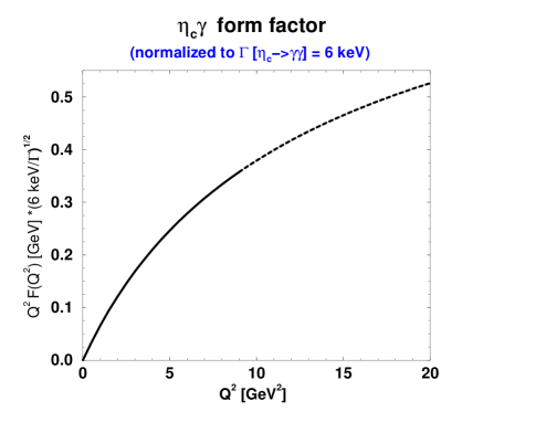
Figure 1: The $\eta_{c}\gamma$ form factor rescaled by $Q^{2}$ and normalized to $\Gamma_{\eta_{c}\to\gamma\gamma}=6$ keV in leading order of the HSA. For $Q^{2}>M^{2}$ (dashed line) the perturbative QCD corrections are expected to become important.

The following conclusions can be drawn: The shape of the form factor predicted by the HSA approach is unique. It can be well approximated by

$$F_{\eta_{c}\gamma}(Q^{2}) \simeq \frac{F(0)}{1+Q^{2}/(M^{2}+2\,\langle\vec{k}_{\perp}^{2}\rangle)}$$ (12)

which takes into account the leading corrections to the collinear approximation, reducing the form factor at $Q^{2}=0$ by order 10%. In our case we have $M^{2}+2\,\langle\vec{k}_{\perp}^{2}\rangle\simeq(3.2~{}{\rm GeV})^{2}$ which is not much larger than the value for the $J/\Psi$ mass that one would have inserted in the VDM approach. Note that eq. (12) may be of particular use for the analysis of the decay width $\Gamma_{\eta_{c}\to\gamma\gamma}$.

The decay constant $f_{\eta_{c}}$ enters the form factor as an overall factor. Thus, in principle one may determine its value from a precise measurement of $F_{\eta_{c}\gamma}$ and/or $\Gamma_{\eta_{c}\to\gamma\gamma}$. For this purpose also the perturbative corrections to the form factor at arbitrary $Q^{2}$ should be taken into account in a consistent way, which is to be analyzed in a forthcoming paper. In this context more precise information from other theoretical approaches (lattice, QCD sum rules) is of course welcome.

References

References

• [1] G.ย P. Lepage and S.ย J. Brodsky, Phys. Rev. D22, 2157 (1980).
• [2] P.ย Kroll and M.ย Raulfs, Phys. Lett. B387, 848 (1996), hep-ph/9605264.
• [3] R.ย Jakob, P.ย Kroll, and M.ย Raulfs, J. Phys. G22, 45 (1996), hep-ph/9410304.
• [4] J.ย Botts and G.ย Sterman, Nucl. Phys. B325, 62 (1989).
• [5] M.ย Wirbel, B.ย Stech, and M.ย Bauer, Z. Phys. C29, 637 (1985).
• [6] Particle Data Group, R.ย M. Barnett etย al., Phys. Rev. D54, 1 (1996).
• [7] R.ย Barbieri, E.ย dโ€™Emilio, G.ย Curci, and E.ย Remiddi, Nucl. Phys. B154, 535 (1979).
• [8] M.ย R. Ahmady and R.ย R. Mendel, Z. Phys. C65, 263 (1995), hep-ph/9401327.
• [9] D.ย S. Hwang and G.-H. Kim, (1997), hep-ph/9703364.
• [10] K.-T. Chao, H.-W. Huang, J.-H. Liu, and J.ย Tang, (1996), hep-ph/9601381.
• [11] E.ย Braaten, Phys. Rev. D28, 524 (1983).