DESY 97-083 ISSN 0418-9833
May 1997
Classical Statistical Mechanics and Landau Damping

Abstract

We study the retarded response function in scalar $\phi^{4}$-theory at finite temperature. We find that in the high-temperature limit the imaginary part of the self-energy is given by the classical theory to leading order in the coupling. In particular the plasmon damping rate is a purely classical effect to leading order, as shown by Aarts and Smit. The dominant contribution to Landau damping is given by the propagation of classical fields in a heat bath of non-interacting fields.

In the high-temperature phase of the standard model of electroweak interactions baryon-number and lepton-number violating processes are in thermal equilibrium [1]. This is of crucial importance for the presently observed cosmological baryon asymmetry and the ‘sphaleron rate’ of baryon-number violation is a corner stone of the theory of baryogenesis.

In order to obtain the sphaleron rate one has to compute a real-time correlation function at finite temperature in a non-abelian gauge theory - a problem which, up to now, could not be solved. Several years ago Grigoriev and Rubakov suggested that the dominant contribution to the sphaleron rate could be obtained by computing the classical time evolution of the gauge fields and averaging over the initial conditions with the Boltzmann weight factor [2]. This classical real-time method has indeed led to an accurate determination of the ‘classical’ sphaleron rate which was shown to be insensitive to the ultraviolet cutoff [3]. The same procedure has been used to study other real-time properties of the SU(2)-Higgs model at finite temperature [4, 5].

The classical real-time method has been questioned for several reasons. One worry concerns the well know ultraviolet divergencies of classical statistical field theory [6, 7]. Another open problem is the role of Landau damping [8, 9], i.e., the loss of energy of quasi-particle excitations in the plasma to the heat bath.

To elucidate the role of classical field theory for finite-temperature quantum field theory, Aarts and Smit have recently studied the plasmon damping rate in scalar $\phi^{4}$-theory [10]. As they have shown, the damping rate is determined by the classical theory to leading order in the coupling. In this paper we extend this analysis by studying the retarded response function in scalar $\phi^{4}$-theory. It turns out that the imaginary part of the self-energy is entirely given by the classical theory in the high-temperature limit to leading order in the coupling. We also calculate the dominant subleading contribution to the plasmon damping rate which is a genuine quantum effect.

Retarded Response Function in the Quantum Theory

We consider scalar $\phi^{4}$-theory at temperature $T=1/\beta$. Perturbation theory is most easily carried out in the imaginary time formalism which is based on the action

$$S = \int_{\beta}dx\left({1\over 2}\partial_{\mu}\phi\partial_{\mu}\phi+{1\over 2}m^{2}\phi^{2}+{1\over 4!}\lambda\phi^{4}+\delta\right)\,,$$ (1)

$$\qquad\int_{\beta}dx=\int_{0}^{\beta}d\tau\int d^{3}x\,.$$

Here $m$ is the plasmon mass,

$$m^{2}={1\over 24}\lambda T^{2}\,,$$ (2)

and $\delta$ stands for counter terms associated with zero-temperature ultraviolet divergencies as well as the resummation at finite temperature [11]. The two-point function

$$D(\tau_{1}-\tau_{2},\vec{x}_{1}-\vec{x}_{2})=\langle\phi(\tau_{1},\vec{x}_{1})\phi(\tau_{2},\vec{x}_{2})\rangle$$ (3)

satisfies the periodic boundary condition $D(0,\vec{x})=D(\beta,\vec{x})$. Hence, its Fourier transform is only defined for the discrete energies given by the Matsubara frequencies $\omega_{n}=2\pi n/\beta$, with $n=0,\pm 1,\pm 2,\ldots$,

$$D(\tau,\vec{x})={1\over\beta}\sum_{n}e^{i\omega_{n}\tau}\int d^{3}xe^{i\vec{p}\vec{x}}D(i\omega_{n},\vec{p})\,.$$ (4)

Analytic continuation yields the function $D(z,\vec{p})$ for complex values of $z$ [14]. This function is related to the self-energy by a Dyson-Schwinger equation,

$$\Pi(z,\vec{p})=D^{-1}(z,\vec{p})-D^{-1}_{0}(z,\vec{p})\,.$$ (5)

Here $D_{0}(z,\vec{p})=1/(z^{2}-\omega_{p}^{2})$, with $\omega_{p}=\sqrt{\vec{p}^{2}+m^{2}}$, is the free two-point function. Along the real axis real and imaginary part of the self-energy are defined by ($\omega=\omega^{*}$),

$$\Pi(\omega\pm i\epsilon,\vec{p})=\Pi_{R}(\omega,\vec{p})\pm i\ \Gamma(\omega,\vec{p})\,.$$ (6)

Knowing $D(z,\vec{p})$ in the complex plane, the various two-point functions can be evaluated by choosing the appropriate path. We are particularly interested in the retarded two-point function which is given by

$$D_{R}^{qu}(t,\vec{p})=\int_{-\infty}^{+\infty}{d\omega\over 2\pi}D(\omega+i\epsilon,\vec{p})e^{-i\omega t}\,.$$ (7)

For small couplings $\lambda$ the self-energy $\Pi(z,\vec{p})$ can be evaluated in perturbation theory. If $D(z,\vec{p})$ has a pole at

$$\bar{z}=\bar{\omega}_{p}-i\bar{\gamma}_{p}\,,$$ (8)

with

$$\bar{\omega}_{p}\simeq\sqrt{\omega_{p}^{2}-\Pi_{R}(\omega_{p},\vec{p})}\,,\quad\bar{\gamma}_{p}\simeq{1\over 2\omega_{p}}\Gamma(\omega_{p},\vec{p})\,,$$ (9)

the integral in Eq. (7) is easily evaluated, and one obtains the ordinary retarded Green’s function,

$$D_{R}^{qu}(t,\vec{p})\simeq-\Theta(t){1\over\bar{\omega}_{p}}\sin(\bar{\omega}_{p}t)e^{-\bar{\gamma}_{p}t}\,.$$ (10)

The retarded two-point function can also be expressed as ensemble average of a product of field operators,

$$iD_{R}^{qu}(t-t^{\prime},\vec{x}-\vec{x}^{\prime})=\mbox{Tr}\left(e^{-\beta\hat{H}}[\hat{\phi}(t,\vec{x}),\hat{\phi}(t^{\prime},\vec{x}^{\prime})]\right)\Theta(t-t^{\prime})\,,$$ (11)

where $\hat{H}$ is the hamilton operator of the theory. Hence, $D_{R}$ describes the response of the system to a perturbation caused by an external current. Adding to the hamiltonian a source term,

$$\hat{H}_{s}(t)=\int d^{3}xj(t,\vec{x})\hat{\phi}(t,\vec{x})\,,$$ (12)

leads to a non-vanishing ensemble average of the field operator. In linear response theory one obtains

$$\langle\hat{\phi}(t,\vec{x})\rangle_{qu} = \mbox{Tr}\left(e^{-\hat{H}}\hat{\phi}(t,\vec{x})\right)$$ (13)

$$= \int dt^{\prime}\int d^{3}x^{\prime}j(t^{\prime},\vec{x^{\prime}})D_{R}(t-t^{\prime},\vec{x}-\vec{x}^{\prime})\,.$$

The finite-temperature two-point functions have been studied in detail in the literature. The self energy $\Pi(z,\vec{p})$ has been calculated in perturbation theory to two-loop order [12, 13]. We will be particularly interested in the damping rate, i.e., the imaginary part. It consists of two parts [14]: the first one, which is present also at zero temperature, is due to the off-shell decay of a scalar particle into three on-shell scalar particles; the second part results from Landau damping, i.e., the scattering of the off-shell scalar particle from the heat bath. The imaginary part of the self-energy reads at two-loop order ($\omega>0$) [13],

$$\Gamma(\omega,\vec{p}) = {\pi\over 6}\lambda^{2}\left(e^{\beta\omega}-1\right)\int d\Phi(\vec{p})\left[\delta(\omega-\omega_{1}-\omega_{2}-\omega_{3})f_{1}f_{2}f_{3}\right.$$ (14)

$$\hskip 85.35826pt+\left.3\delta(\omega+\omega_{1}-\omega_{2}-\omega_{3})(1+f_{1})f_{2}f_{3}\right]\,,$$

$$\Gamma(-\omega,\vec{p}) = -\Gamma(\omega,\vec{p})\,,$$ (15)

where $d\Phi(\vec{p})$ is the integration measure,

$$d\Phi(\vec{p})={d^{3}q_{1}\over(2\pi)^{3}2\omega_{1}}{d^{3}q_{2}\over(2\pi)^{3}2\omega_{2}}{d^{3}q_{3}\over(2\pi)^{3}2\omega_{3}}(2\pi)^{3}\delta(\vec{p}-\vec{q_{1}}-\vec{q_{2}}-\vec{q_{3}})\,,$$ (16)

and $f$ is the Bose-Einstein distribution function,

$$f(\omega)={1\over e^{\beta\omega}-1}\,.$$ (17)

The two contributions to $\Gamma(\omega,\vec{0})$ have thresholds at $\omega=3m$ and $\omega=m$, respectively. Only the first term is present at zero temperature. At temperatures $T\gg m$ both terms are dominated by interactions with the heat bath, i.e., by Landau damping.

Retarded Response Function in the Classical Theory

The retarded response function can also be studied in the classical theory at finite temperature. The classical hamiltonian is the sum of the free hamiltonian, a self-interaction term and a source term,

$$H=\int d^{3}x\left({1\over 2}\pi^{2}+{1\over 2}(\vec{\partial}\phi)^{2}+{1\over 2}m^{2}_{cl}\phi^{2}+{1\over 4!}\lambda\phi^{4}+j\phi\right)\,,$$ (18)

where $j(t,\vec{x})$ is an external souce. Note, that $m_{cl}=1/l_{cl}$ is an inverse length. It is different from the plasmon mass $m$ given in Eq. (2). The ensemble average of the classical field is then given by

$$\langle\phi(t,\vec{x})\rangle_{cl}={1\over Z}\int{\cal D}\pi{\cal D}\phi e^{-H(\pi,\phi)}\phi(t,\vec{x})\,,$$ (19)

with

$$Z=\int{\cal D}\pi{\cal D}\phi e^{-H(\pi,\phi)}\,.$$ (20)

Here $\phi(t,\vec{x})$ is the solution of the equations of motion

$$\dot{\phi}(t,\vec{x}) = \pi(t,\vec{x})\,,$$

$$\dot{\pi}(t,\vec{x}) = \Delta\phi(t,\vec{x})-m^{2}_{cl}\phi(t,\vec{x})-{\lambda\over 3!}\phi^{3}(t,\vec{x})-j(t,\vec{x})\,,$$ (21)

with the initial conditions

$$\phi(t_{0},\vec{x})=\phi(\vec{x})\,,\quad\pi(t_{0},\vec{x})=\pi(\vec{x})\,.$$ (22)

In Eqs. (19) and (20) the domain of integration is the space of initial conditions.

The solution of the equations of motion satisfies the integral equation ($t,t^{\prime}>t_{0},x\equiv(t,\vec{x})$),

$$\phi(x;j)=\phi_{0}(x)+\int d^{4}x^{\prime}D_{R}(x-x^{\prime})\left({\lambda\over 3!}\phi^{3}(x^{\prime};j)+j(x^{\prime})\right)\,.$$ (23)

Here $\phi_{0}$ is the solution of the free equations of motion which satisfies the boundary condition, and $D_{R}$ is the retarded Green’s function,

$$D_{R}(t,\vec{x})=-\int{d^{3}q\over(2\pi)^{3}}e^{i\vec{q}\vec{x}}\Theta(t){1\over\omega_{q}}\sin(\omega_{q}t)\,.$$ (24)

The classical solution can be expanded in powers of the external current. The term linear in $j(x)$ is given by (cf. (13))

$$\phi(x)=\int d^{4}x^{\prime}j(x^{\prime})H_{R}(x-x^{\prime})\,,$$ (25)

where

$$H_{R}(x-x^{\prime})=\left.{\delta\phi(x;j)\over\delta j(x^{\prime})}\right|_{j=0}$$ (26)

depends on the initial conditions $\phi(\vec{x})$ and $\pi(\vec{x})$. From Eqs. (23) and (26) one reads off the integral equation which determines $H_{R}$,

$$H_{R}(x-x^{\prime})=D_{R}(x-x^{\prime})+{1\over 2}\lambda\int d^{4}yD_{R}(x-y)\phi^{2}(y;0)H_{R}(y-x^{\prime})\,.$$ (27)

In order to obtain the finite-temperature retarded response function, i.e., the classical analogue of $D_{R}^{qu}$ (cf. (11)), one has to compute the ensemble average with respect to the initial conditions. This yields

$$\langle\phi(x)\rangle_{cl}=\int d^{4}x^{\prime}j(x^{\prime})D_{R}^{cl}(x-x^{\prime})\,,$$ (28)

where

$$D_{R}^{cl}(x-x^{\prime})=\langle H_{R}(x-x^{\prime})\rangle_{cl}={1\over Z}\int{\cal D}\phi{\cal D}\pi e^{-\beta H}H_{R}(x-x^{\prime})\,.$$ (29)

The classical retarded response function $D_{R}^{cl}$ can be evaluated by first expanding the solution (27) for $H_{R}$ in powers of $\lambda$ (cf. Fig. 1) and then performing the thermal average for each term.

Figure 1: The response function $H_{R}$ expanded in powers of the classical field. Full lines denote retarded Green’s functions $G_{R}$

This requires the evaluation of the thermal n-point functions

$$\langle\phi^{2}(x_{1})\ldots\phi^{2}(x_{2n})\rangle_{cl}\,.$$ (30)

Consider first the thermal average with the free Hamiltonian $H_{0}$. The corresponding two-point function reads [15, 10]

$$S(t-t^{\prime},\vec{x}-\vec{x}^{\prime})=\langle\phi(x)\phi(x^{\prime})\rangle_{cl}^{0}\\ =T\int{d^{3}q\over(2\pi)^{3}}e^{i\vec{k}(\vec{x}-\vec{x}^{\prime})}{1\over\omega_{k}^{2}}\cos(\omega_{k}(t-t^{\prime}))\,.$$

For higher n-point functions one has

$$\langle\phi^{2}(x_{1})\ldots\phi^{2}(x_{2n})\rangle_{cl}^{0}=2^{n}S^{2}(x_{1}-x_{2})\ldots S^{2}(x_{2n-1}-x_{2n})+\mbox{permutations}\,.$$ (31)

From Fig. 1 it is clear that the response function obtained after thermal averaging with $H_{0}$ satisfies a Dyson-Schwinger equation (cf. Fig. 2),

$$\bar{D}_{R}^{cl}(x-x^{\prime})=D_{R}(x-x^{\prime})+\int d^{4}yd^{4}y^{\prime}D_{R}(x-y)\bar{\Pi}(y-y^{\prime})_{cl}\bar{D}_{R}^{cl}(y^{\prime}-x^{\prime})\,.$$ (32)

Figure 2: Dyson-Schwinger equation for the retarded response function $\bar{D}_{R}^{cl}$

The terms in the perturbative expansion for the self-energy $\Pi(x)$ are shown in Fig. 3 up to ${\cal O}(\lambda^{2})$.

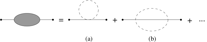
Figure 3: Perturbative expansion for the self-energy $\Pi$. Dashed lines denote thermal two-point functions $S$.

The contribution ${\cal O}(\lambda)$ (Fig. 3a) is linearly divergent and can be removed by a mass renormalization yielding the counter term [10]

$$\delta m^{2}_{1}={1\over 2}\lambda S(0,\vec{0})={1\over 2}\lambda T\int{d^{3}q\over(2\pi)^{3}}{1\over\omega_{q}^{2}}\,.$$ (33)

The contribution ${\cal O}(\lambda^{2})$ (Fig. 3b) is logarithmically divergent and can be rendered finite by a further mass renormalization

$$\delta m^{2}_{2}=-{1\over 6}\lambda^{2}\beta\int d^{3}xS^{3}(0,\vec{x})=-{4\over 3}\lambda^{2}T^{2}\int d\Phi(\vec{0}){1\over\omega_{1}\omega_{2}\omega_{3}}\,.$$ (34)

Contributions of higher order in $\lambda$ are all finite.

We are interested in the damping rate, i.e., the imaginary part of the self-energy which is finite. Using Eqs. (24) and (DESY 97-083 ISSN 0418-9833 May 1997 Classical Statistical Mechanics and Landau Damping) one easily obtains for the self-energy to order $\lambda^{2}$,

$$\bar{\Pi}(\omega,\vec{p})_{cl} = \int dtd^{3}x\ e^{i\omega t}e^{-i\vec{p}\vec{x}}\ \bar{\Pi}(t,\vec{x})_{cl}$$ (35)

$$= {1\over 2}\lambda^{2}T^{2}\sum_{\eta_{1},\eta_{2},\eta_{3}}\eta_{1}\int d\Phi(\vec{p})\ {1\over\omega_{2}\omega_{3}}{1\over\omega+\eta_{1}\omega_{1}+\eta_{2}\omega_{2}+\eta_{3}\omega_{3}+i\epsilon}\,,$$

where $\eta_{i}=\pm 1$, $i=1,\ldots,3$.

From Eq. (35) one obtains for the imaginary part of the self-energy ($\omega>0$),

$$\bar{\Gamma}(\omega,\vec{p})_{cl}={\pi\over 2}\lambda^{2}T^{2}\int d\Phi(\vec{p}){1\over\omega_{1}\omega_{2}\omega_{3}}\left[\omega_{1}\delta(\omega-\omega_{1}-\omega_{2}-\omega_{3})+\omega\delta(\omega+\omega_{1}-\omega_{2}-\omega_{3})\right]\,.$$ (36)

We can now compare the classical damping rate $\bar{\Gamma}_{cl}$ with the damping rate $\Gamma$ of the full quantum theory as given by Eq. (14). At very high temperatures, i.e., $T\gg m$, the Bose-Einstein distribution function becomes

$$f(\omega)\simeq{T\over\omega}\gg 1\,.$$ (37)

Inserting this approximation into Eq. (14) yields precisely Eq. (36). Hence, in the high-temperature limit, where number densities are very high, the damping rates are given by the classical theory to leading order. In particular the on-shell plasmon damping rate reads

$$\gamma={1\over 2}l_{qu}\Gamma(m,\vec{0})\\ ={1\over 1536\pi}l_{qu}\lambda^{2}T^{2}\,,$$

where

$$l_{qu}=\hbar\left({\hbar\lambda\over 24}T^{2}\right)^{-1/2}$$ (38)

is the Compton wave length associated with the plasmon mass (2). Replacing $l_{qu}$ by $l_{cl}$ yields the classical plasmon rate. This is the result of Aarts and Smit [10]. As our analysis shows, this result extends to the full off-shell imaginary part of the self-energy in the high-temperature limit.

Use of the Classical Theory

So far we have performed the thermal average in the classical theory with respect to the free hamiltonian $H_{0}$, and we have calculated the self-energy $\bar{\Pi}_{cl}$ to order $\lambda^{2}$. Higher orders in the expansion of $H_{R}$ (cf. Fig. 1) and, furthermore, the thermal average with the full hamiltonian $H$ rather than $H_{0}$ yield corrections of higher order in $\lambda$.

However, if one is interested in the classical theory as a tool to evaluate the leading contribution of the quantum theory, the full result of the classical theory is irrelevant. Consider again the two-loop expression (14) for $\Gamma(\omega,\vec{p})$. In the high-temperature limit terms proportional to the product of two Bose-Einstein distribution functions $f(\omega_{i})f(\omega_{j})$ dominate. This contribution is given by the classical theory. Contributions to $\Gamma(\omega,\vec{p})$ proportional to a single distribution function $f(\omega_{i})$ are subdominant. Such terms do not occur in the classical theory. They lead to the following correction for the on-shell plasmon damping rate,

$$\delta\Gamma(m,\vec{0})=\pi\lambda T\int d\Phi(\vec{0}){1\over\omega_{3}}\delta(m+\omega_{1}-\omega_{2}-\omega_{3})\,,$$ (39)

which yields

$$\delta\gamma={1\over 512\pi^{3}}\hbar\lambda^{2}\ln{(\hbar\lambda)}T\,.$$ (40)

On dimensional grounds such a correction cannot appear in the classical theory.

In summary, we have shown that in the high-temperature limit the imaginary part of the self-energy is determined by the classical theory to leading order in the coupling, whereas the dominant subleading contribution is a genuine quantum effect. In order to obtain the leading order contribution to damping rates it is sufficient to perform the thermal average with respect to the initial conditions with the free hamiltonian. Such a simplification may be useful in numerical simulations for damping rates.

We would like to thank D. Bödeker, A. Patkós and J. Polonyi for valuable discussions and comments.

References

[1] V. A. Kuzmin, V. A. Rubakov and M. E. Shaposhnikov,
Phys. Lett. B155 (1985) 36
[2] D. Yu. Grigoriev and V. A. Rubakov, Nucl. Phys. B299 (1988) 67
[3] J. Ambjorn and A. Krasnitz, Phys. Lett. B362 (1995) 97
[4] G. D. Moore and N. Turok, preprint DAMTP 96-77,
hep-ph/9608350
[5] W. H. Tang and J. Smit, preprint ITFA-97-02, hep-ph/9702017
[6] D. Bödeker, L. McLerran and A. Smilga, Phys. Rev. D52
(1995) 4675
[7] D. Bödeker, Nucl. Phys. B486 (1997) 500
[8] P. Arnold and L. McLerran, Phys. Rev. D36 (1987) 581
[9] P. Arnold, D. Son and L. G. Yaffe, preprint UW/PT-96-19,
hep-ph/9609481
[10] G. Aarts and J. Smit, Phys. Lett. B393 (1997) 395
[11] L. Dolan and R. Jackiw, Phys. Rev. D9 (1974) 3320
[12] R. R. Parwani, Phys. Rev. D45 (1992) 4695
[13] E. Wang and U. Heinz, Phys. Rev. D53 (1996) 899
[14] H. A. Weldon, Phys. Rev. D28 (1983) 2007
[15] G. Parisi, Statistical Field Theory (Addison-Wesley,
1988, New York), p. 309