IC/97/49

hep-ph/9705451

THE NEUTRINO MAGNETIC MOMENT AND TIME VARIATIONS OF THE SOLAR NEUTRINO FLUX

E.Kh. Akhmedov
International Centre for Theoretical Physics
Strada Costiera 11, I-34100 Trieste, Italy

The present status of the neutrino magnetic moment solutions of the solar neutrino problem is summarized. After a brief review of the basics of the neutrino spin and spin–flavor precession I discuss the experimental data and show how the neutrino resonant spin–flavor precession (RSFP) mechanism can naturally account for sizeable time variations in the Homestake signal and no observable time variations in the Kamiokande and gallium experiments. Fits of the existing data and predictions for the forthcoming solar neutrino experiments are also discussed. In the last section I summarize the objections to the RSFP mechanism that are frequently put forward and comment on them.

1 Introduction

The combined data of all the currently operating solar neutrino experiments strongly suggest that the observed deficiency of the solar neutrino flux is due to some unconventional neutrino properties and not to astrophysics. The analysis [1] also shows that the standard solar models which take into account the element diffusion are in a very impressive agreement with the high-accuracy helioseismological data whereas the so-called unconventional solar models grossly disagree with them. This lends further support to the point of view that it is some new neutrino physics and not our poor knowledge of the solar physics that is responsible for the solar neutrino problem.

The main neutrino–physics explanations of the problem that have been discussed so far are neutrino oscillations (in solar matter or in vacuum), neutrino decay, and neutrino magnetic moments. The relevant process that is caused by the neutrino magnetic moment is the neutrino spin precession in the solar magnetic field. By now, the neutrino decay explanation has been ruled out: It predicts stronger depletion of the lower-energy neutrino flux, in direct contradiction with the data. Vacuum and matter–enhanced oscillations (the MSW effect) are in a good shape [2]; the latter is at the moment the most popular candidate for the solution of the solar neutrino problem. It is generally believed that the neutrino magnetic moment is strongly disfavored by the present data, if not excluded. I will try to convince you that this is wrong. It may well be that the magnetic moment solutions soon will be ruled out by the Super–Kamiokande and SNO experiments; however, at the moment they are in a perfectly good agreement with all the existing data.

The neutrino magnetic moment can account for both the observed deficiency of the solar neutrino flux and the time variation of the signal. The time dependence may be caused by time variations of the magnetic field in the convective zone of the sun. Some evidence for such time variations exists in the Homestake data, whereas no time variations were observed in Kamiokande and gallium experiments, at least within their experimental errors. I will explain that this may be a very natural consequence of the neutrino transition (flavor-off-diagonal) magnetic moment.

2 Neutrino spin precession

The idea that neutrino magnetic moment may have something to do with the deficiency of the solar neutrino flux was first put forward by Cisneros more than 25 years ago [3]. His point was very simple: If the electron neutrino has a magnetic moment, its spin will precess in a transverse magnetic field which means that a fraction of the left-handed neutrinos $\nu_{eL}$ will be converted into the right-handed $\nu_{eR}$. These $\nu_{eR}$ are sterile – they do not take part in the usual weak interactions and therefore cannot be detected, which explains the deficiency of the observed flux. It is not difficult to find the probability of the $\nu_{eL}\to\nu_{eR}$ transition:

$$P(\nu_{eL}\to\nu_{eR};r)=\sin^{2}\left(\int_{0}^{r}\mu B_{\bot}(r^{\prime})\,dr^{\prime}\right)\,.$$ (1)

Here $\mu$ is the neutrino magnetic moment and $B_{\bot}(r)$ is the transverse magnetic field strength, $r$ being the coordinate along the neutrino path. This formula is valid for an arbitrary magnetic field profile $B_{\bot}(r)$. There are two important things to be noticed. First, the transition probability does not depend on the neutrino energy, i.e. neutrinos of all the energies experience the same degree of the $\nu_{eL}\to\nu_{eR}$ conversion, and the spectrum of the surviving $\nu_{eL}$’s is undistorted. Second, the amplitude of the precession is unity: If the neutrino magnetic moment is large enough, the transverse magnetic field is strong and extended enough, in principle a beam of the $\nu_{eL}$’s can be fully converted into the $\nu_{eR}$ beam.

In his paper [3] Cisneros assumed that there is a strong constant in time magnetic field in the core of the sun, and this field causes the neutrino spin precession. However, he did not take into account the matter effects on the precession, which can be quite strong in the dense solar core. At that time it was simply not known that matter can influence neutrino propagation significantly. The solar matter effects on the neutrino spin precession were considered by Voloshin, Vysotsky and Okun (VVO) [4] and by Barbieri and Fiorentini [5]. VVO also made the following important observation: There is a strong toroidal magnetic field in the convective zone of the sun, and this field varies in time with the 11-year periodicity. If one assumes that at the maxima of solar activity, when one observes the maximum number of sunspots, the magnetic field is strongest, one can expect to see the smallest flux of solar neutrinos at these periods. This is because the neutrino spin precession converting the $\nu_{eL}$’s into unobservable $\nu_{eR}$’s should be most efficient for strongest magnetic fields. In other words, the observed solar neutrino flux should vary in time in anticorrelation with solar activity. Another interesting point made by VVO was the following: It is known that the toroidal magnetic field has opposite directions in the northern and southern hemispheres of the sun. This means that it must vanish near the solar equator. The orbit of the earth is inclined by $7^{\circ}15^{\prime}$ to ecliptic, therefore twice a year (in the beginning of June and in the beginning of December) the solar core is seen from the earth through the equatorial gap in the toroidal magnetic field of the sun. One can expect the solar neutrinos observed on the earth during these periods to be unaffected by the solar magnetic filed and therefore their flux not to be suppressed even in the periods of high solar activity. This should lead to very peculiar semiannual variations of the solar neutrino signal. I will discuss the experimental status of the time variations of the solar neutrino flux later on.

In the presence of matter one cannot find the precession probability for arbitrary magnetic field and matter density profiles in a closed analytical form. However, in the simplest case of the uniform magnetic field and constant matter density such an expression can be readily found [4, 5]:

$$P(\nu_{eL}\to\nu_{eR};r)=\frac{(2\mu B_{\bot})^{2}}{[\sqrt{2}G_{F}(N_{e}-N_{n}/2)]^{2}+(2\mu B_{\bot})^{2}]}\sin^{2}\left(\frac{1}{2}\sqrt{D_{1}}\,r\right)\,.$$ (2)

Here $G_{F}$ is the Fermi constant, $N_{e}$ and $N_{n}$ are the electron and neutron number densities, and $D_{1}$ in the argument of the sine is the denominator of the pre-sine factor. Comparing this expression with eq. (1), we see an important difference: in matter the precession amplitude (i.e. the pre-sine factor) is always less than one. The reason for that is very simple. In vacuum the left-handed and right-handed components of a Dirac neutrino are degenerate, so the precession relates the states of the same energy and therefore proceeds with the amplitude equal to unity. In matter this is no longer true – left-handed neutrinos experience coherent forward scattering on the particles of the medium, i.e. receive some mean potential energy, whereas the sterile right-handed neutrinos have zero potential energy. This results in an energy splitting of the $\nu_{eL}$ and $\nu_{eR}$. The neutrino spin precession now relates the states of different energy and its amplitude is therefore always less than one. If the interaction that mixes the $\nu_{eL}$ and $\nu_{eR}$, the Zeeman energy $\mu B_{\bot}$, is much smaller than the energy splitting $\sqrt{2}G_{F}(N_{e}-N_{n}/2)$, the precession is strongly suppressed.

There is one thing that is common for eqs. (1) and (2): in both cases the transition probability does not depend on the neutrino energy, i.e. neutrinos of all the energies experience the same degree of the $\nu_{eL}\to\nu_{eR}$ conversion. This is an important property of the neutrino spin precession that holds for arbitrary magnetic field and matter density profiles.

3 Resonant spin-flavor precession of neutrinos

3.1 General features

If the lepton flavor is not conserved, neutrinos may have flavor-off-diagonal (transition) magnetic moments. Such magnetic moments would cause, e.g., radiative neutrino decays $\nu_{2}\to\nu_{1}+\gamma$. In transverse magnetic fields neutrinos with transition magnetic moments will experience a very special type of the spin precession: their spin will rotate with their favor changing simultaneously [6, 4]. This is called the spin–flavor precession (SFP). For example, if neutrinos are the Dirac particles, $\nu_{eL}$ can be rotated into sterile $\nu_{\mu R}$. Majorana neutrinos cannot have ordinary magnetic moments because of CPT invariance; however, they can have the transition magnetic moments. For Majorana neutrinos the SFP converts left-handed neutrinos of a given flavor into right-handed antineutrinos of a different flavor. The latter are not sterile – they are just the usual antineutrinos which take part in the standard weak interactions. It is not difficult to find the probability of the SFP in vacuum. Consider, for example, the $\nu_{eL}\leftrightarrow\bar{\nu}_{\mu R}$ transitions. In the case of the uniform magnetic field the transition probability for relativistic neutrinos is

$$P(\nu_{eL}\to\bar{\nu}_{\mu R};r)=\frac{(2\mu B_{\bot})^{2}}{(\Delta m^{2}/2E)^{2}+(2\mu B_{\bot})^{2}}\sin^{2}\left(\frac{1}{2}\sqrt{D_{2}}\,r\right)\,.$$ (3)

Here $\mu$ is now the transition magnetic moment, $\mu\equiv\mu_{\nu_{e}\nu_{\mu}}$, $\Delta m^{2}=m_{\nu_{\mu}}^{2}-m_{\nu_{e}}^{2}$, and $D_{2}$ is the denominator of the pre-sine factor. For simplicity I have assumed here that the $\nu_{e}$ and $\nu_{\mu}$ are mass eigenstates; I will discuss the case when both transition magnetic moment and neutrino mass mixing are present later.

For some time the SFP of neutrinos did not attract much attention. The reason for this was that its probability is suppressed even in vacuum. Indeed, neutrinos of different flavor are expected to have different masses, so even in the absence of matter we now have the transitions between the non-degenerate neutrino states. The kinetic energy difference of the relativistic neutrinos is $\Delta m^{2}/2E$; if this energy difference is small compared to the “Zeeman energy” $\mu B_{\bot}$ the precession amplitude is suppressed. However, in 1988 it was realized that in matter the situation changes drastically [7, 8]. Left-handed neutrinos of a given flavor and right-handed neutrinos or antineutrinos of a different flavor experience different coherent forward scattering on the particles of the medium, and so there is a potential energy difference which has to be subtracted from the kinetic energy difference in the expression for the transition probability:

$$P(\nu_{eL}\to\bar{\nu}_{\mu R};r)=\frac{(2\mu B_{\bot})^{2}}{(\Delta m^{2}/2E-\sqrt{2}G_{F}N_{\rm eff})^{2}+(2\mu B_{\bot})^{2}}\sin^{2}\left(\frac{1}{2}\sqrt{D_{3}}\,r\right)\,.$$ (4)

Here $D_{3}$ is the denominator of the pre-sine factor and $N_{\rm eff}$ depends on the nature of the neutrinos:

$$N_{\rm eff} = N_{e}-N_{n}/2\;\;{\mbox{\rm for Dirac neutrinos}}$$ (5)

$$= N_{e}-N_{n}\;\;\;\;\;{\mbox{\rm for Majorana neutrinos}}$$

Now, for a given $\Delta m^{2}$ and any value of the neutrino energy $E$ there is a certain value of $N_{\rm eff}$ for which the potential energy difference $\sqrt{2}G_{F}N_{\rm eff}$ exactly cancels the kinetic energy difference $\Delta m^{2}/2E$, and the amplitude of the SFP becomes equal to unity, no matter how small the transition magnetic moment $\mu$ and how weak the magnetic field $B_{\bot}$. The precession amplitude as a function of $N_{\rm eff}$ has a typical resonant behavior, i.e. matter can resonantly enhance the neutrino SFP. Of course, having a large precession amplitude is not sufficient for the precession probability to be large; the phase of the sine in eq. (4) should also be not too small. This puts a lower limit on the product $\mu B_{\bot}$. In the matter with varying density the lower bound on $\mu B_{\bot}$ is imposed by the adiabaticity condition which I will shortly discuss.

The resonant spin–flavor precession (RSFP) of neutrinos in matter is very similar to the resonant enhancement of the neutrino oscillations in matter – the celebrated MSW effect [9, 10]. In fact, the mathematics describing the neutrino oscillations and spin (or spin–flavor) precession is just the same (although there are some important differences in the physics involved). This is not by accident, of course. The processes of both types in the simplest case of two neutrino species involved reduce to a well-known quantum mechanical problem of a two-level system in an external field; one can find a discussion of this problem in any textbook of quantum mechanics. The evolution of the system is governed by the Shroedinger-like equation

$$i\frac{d}{dr}\left(\begin{array}[]{l}\nu_{i}\\ \nu_{j}\end{array}\right)~{}=~{}\left(\begin{array}[]{cc}E_{i}&V_{ij}\\ V_{ij}^{*}&E_{j}\end{array}\right)\left(\begin{array}[]{l}\nu_{i}\\ \nu_{j}\\ \end{array}\right)$$ (6)

Here $\nu_{i}$ and $\nu_{j}$ are the probability amplitudes of finding the corresponding neutrino at a point $r$, $E_{i}$ and $E_{j}$ are the energies of the neutrinos in the absence of mixing, and $V_{ij}$ is the mixing interaction. The weak eigenstate neutrinos $\nu_{i}$ and $\nu_{j}$ can be of the same or different flavor and of the same of different chirality, depending on the process in question. For the neutrino spin precession they are of the same flavor but different chirality, for the neutrino oscillations they are of different flavor and the same chirality, and for the SFP they are of different flavor and different chirality. The mixing interaction $V_{ij}$ also depends on the process in question. For the neutrino spin or spin–flavor precession it is $\mu B_{\bot}$ where $\mu$ is the ordinary or transition magnetic moment respectively; for the neutrino oscillations $V_{ij}=(\Delta m_{ij}^{2}/4E)\sin 2\theta_{0}$ where $\theta_{0}$ is the mass mixing angle (i.e. the angle that relates mass eigenstates with flavor eigenstates). For relativistic neutrinos, the diagonal matrix elements of the effective Hamiltonian in eq. (6) are $E_{i}\simeq E+m_{i}^{2}/2E+V(\nu_{i})$ where $V(\nu_{i})$ is the matter-induced mean potential energy of the neutrino $\nu_{i}$ [10]:

$$V(\nu_{eL})=-V({\bar{\nu}}_{eR})=\sqrt{2}G_{F}(N_{e}-N_{n}/2)\,,$$ (7)

$$V(\nu_{\mu L},\nu_{\tau L})=-V(\bar{\nu}_{\mu R},\bar{\nu}_{\tau R})=\sqrt{2}G_{F}(-N_{n}/2)\,.$$ (8)

For sterile right-handed neutrinos and their left-handed antiparticles $V(\nu_{i})=0$.

The transition probabilities depend on the difference of the phases of the neutrino states. This means that it is only the difference of the diagonal elements of the effective Hamiltonian in eq. (6) (and not the diagonal elements themselves) that matters:

$$\Delta E_{ij}=\Delta m_{ij}^{2}/2E+V(\nu_{i})-V(\nu_{j})\,.$$ (9)

Thus, the neutrino energy $E$ enters into the evolution equation only through the parameter $\Delta m_{ij}^{2}/2E$. For the neutrinos of the same flavor $\Delta m_{ij}^{2}=0$; this explains why the transition probability for the ordinary (flavor–conserving) neutrino spin precession is independent of the neutrino energy. The effective potential energy term $\sqrt{2}G_{F}N_{\rm eff}$ in eq. (4) is nothing but the difference $V(\nu_{i})-V(\nu_{j})$ [compare eqs. (5), (7) and (8)].

The transition probabilities for the neutrino spin and spin–flavor precession in the absence of matter or in a matter of constant density, (1)–(4), can be easily obtained from the evolution equation (6). However in general, in a medium with arbitrary matter density and magnetic field profiles, no analytical closed–form expression for the transition probability can be obtained. In this case one has to solve eq. (6) numerically, which is quite straightforward. However, even without performing any numerical calculations one can get an important insight into the evolution of the neutrino system in the adiabatic approximation. Consider, for example, the SFP – induced transitions $\nu_{eL}\leftrightarrow\bar{\nu}_{\mu R}$. At any point $r$ one can diagonalize the effective Hamiltonian in eq. (6) and find the instantaneous eigenstates

$$\nu_{A} = \cos\theta\;\nu_{eL}+\sin\theta\;\bar{\nu}_{\mu R}$$

$$\nu_{B} = -\sin\theta\;\nu_{eL}+\cos\theta\;\bar{\nu}_{\mu R}$$ (10)

where the mixing angle $\theta$ is defined through

$$\tan 2\theta=\frac{2\mu B_{\bot}}{\sqrt{2}G_{F}(N_{e}-N_{n})-\Delta m^{2}/2E}\,.$$ (11)

Thus the neutrino eigenstates in matter and magnetic fileds are the linear combinations of the neutrinos of different flavor and chirality. It should be clearly understood that the mixing angle $\theta$ in eqs. (10) and (11) has nothing to do with the usual mixing angle $\theta_{0}$ that governs the neutrino oscillations. For the moment I assume $\theta_{0}=0$.

The resonance condition for the SFP is

$$\sqrt{2}G_{F}(N_{e}-N_{n})=\Delta m^{2}/2E\,.$$ (12)

At the resonance point the mixing angle $\theta=\pi/4$ and the amplitude of the SFP in eq. (4) becomes equal to unity (remember that $N_{\rm eff}=N_{e}-N_{n}$ for Majorana neutrinos). The resonance condition (12) is very similar to that for the MSW effect [9, 10]

$$\sqrt{2}G_{F}N_{e}=(\Delta m^{2}/2E)\cos 2\theta_{0}\,.$$ (13)

The main difference is the $-N_{n}$ term which is due to the neutral current interactions of neutrinos with matter. It is absent in eq. (13) but enters into eq. (12) because the SFP, unlike the neutrino oscillations, is sensitive to the neutral currents. The resonance of the SFP takes place in the $\nu_{eL}\leftrightarrow\bar{\nu}_{\mu R}$ channel if $\Delta m^{2}\equiv m_{\nu_{\mu}}^{2}-m_{\nu_{e}}^{2}>0$ and in the $\bar{\nu}_{eR}\leftrightarrow\nu_{\mu L}$ channel if $\Delta m^{2}<0$. I will be assuming that $\Delta m^{2}>0$.

Consider the variation of the mixing angle $\theta$ along the path of the solar neutrinos. In the core of the sun where they are born the density is high. Assume that it is much larger than the resonance density defined through eq. (12). Then the denominator of eq. (11) is large, i.e. the mixing angle is small: $\theta(r\simeq 0)\simeq 0$. With decreasing density the mixing angle $\theta$ increases; it reaches $\pi/4$ at the resonance point and continues to increase. Close to the surface of the sun the matter density is very small and one can neglect it as compared to the $\Delta m^{2}/2E$ term in the denominator of eq. (11). At the same time, the magnetic field strength decreases towards the surface of the sun, so at $r=R_{\odot}$ the tangent of $2\theta$ is a small negative number, i.e. $\theta\simeq\pi/2$. Thus, as neutrino propagates from the core of the sun to its surface, $\theta$ changes from $\simeq 0$ to $\simeq\pi/2$, passing through $\pi/4$ at the resonance point.

Consider now the evolution of the $\nu_{eL}$’s in the sun. Since $\theta(r\simeq 0)\simeq 0$, it follows from eq. (10) that a $\nu_{eL}$ born in the core of the sun nearly coincides with one of the neutrino matter eigenstates, namely $\nu_{A}$. If the matter density changes slowly enough (adiabatically) along the neutrino path, the neutrino system has enough time to adjust itself to the changing external conditions and the eigenstate $\nu_{A}$ will propagate in matter and magnetic field as $\nu_{A}$ without being converted into $\nu_{B}$. However, the composition of the eigenstates $\nu_{A}$ and $\nu_{B}$ changes along the neutrino path since the mixing angle $\theta$ changes. In particular, at the surface of the sun where $\theta\simeq\pi/2$ the $\nu_{A}$ practically coincides with the $\bar{\nu}_{\mu R}$. This means that we have a complete (or almost complete) adiabatic conversion of $\nu_{eL}$ into $\bar{\nu}_{\mu R}$ in the sun. This phenomenon is very similar to the $\nu_{eL}\to\nu_{\mu L}$ conversion due to the MSW effect. In fact, this is nothing but the well known Landau–Zener effect. The energy levels of a quantum mechanical system cross in the absence of the mixing interaction. However the mixing leads to an avoided level crossing. If the neutrino starts at high densities as the $\nu_{eL}$ which coincides with the higher–energy eigenstate $\nu_{A}$ and remains on the higher–energy branch while propagating to the low densities, it will end up as the $\bar{\nu}_{\mu R}$.

Now, how can one quantify the adiabaticity condition? This is the condition that the external parameters change slowly enough along the neutrino trajectory so that the “jumps” between the $\nu_{A}$ and $\nu_{B}$ states are suppressed. One can show that the adiabaticity condition is most restrictive in the vicinity of the resonance. It can be formulated there as the requirement that at least one precession length $l_{prec}=\pi/\mu B_{\bot}$ fit into the resonance width $\Delta r$ which is defined as the spatial width of the resonance at half height. More precisely,

$$\lambda_{\rm RSFP}\equiv\pi\frac{\Delta r}{l_{prec}}=8\frac{E}{\Delta m^{2}}\,(\mu B_{\bot r})^{2}\,L_{\rm eff}>1\,.$$ (14)

Here $B_{\bot r}$ is the magnetic field strength at the resonace and $L_{\rm eff}=|1/N_{\rm eff}(dN_{\rm eff}/dr)|_{r}^{-1}$ is the effective matter density scale height (the distance over which $N_{\rm eff}$ varies significantly). In the sun, for $0.1R_{\odot}\buildrel<\over{{}_{\sim}}r\buildrel<\over{{}_{\sim}}0.9R_{\odot}$, the scale height $L_{\rm eff}\simeq 0.1R_{\odot}$. Notice that $\lambda_{\rm RSFP}$ is proportional to $(\mu B_{\bot})^{2}$ so that the adiabaticity condition puts a lower bound on the product of the neutrino transition magnetic moment and magnetic field strength at the resonance.

It is instructive to compare eq. (14) with the adiabaticity condition of the MSW effect:

$$\lambda_{\rm MSW}=\frac{\sin^{2}2\theta_{0}}{\cos 2\theta_{0}}\,\frac{\Delta m^{2}}{2E}L_{\rm eff}>1\,.$$ (15)

We see that the energy dependence of the two adiabaticity parameters is quite different: $\lambda_{\rm RSFP}\propto E$ whereas $\lambda_{\rm MSW}\propto E^{-1}$. Therefore one could hope to be able to experimentally distinguish the RSFP from the MSW effect by the distortions they cause to the solar neutrino spectrum. Unfortunately, in reality the situation is much more complicated. The RSFP adiabaticity parameter depends crucially on the magnetic field strength at the resonance $B_{\bot r}$. Since the solar magnetic field is not uniform, $B_{\bot}=B_{\bot}(r)$, the value $B_{\bot r}$ depends on the resonance coordinate which in turn depends on the neutrino energy $E$ through the resonance condition (12). Thus, the adiabaticity parameter $\lambda_{\rm RSFP}$ has an additional implicit neutrino energy dependence entering through $B_{\bot r}$. Since the profile of the solar magnetic field is essentially unknown the distortion of the energy spectrum of the solar neutrinos cannot be unambiguously predicted. In particular, one cannot be sure that the RSFP of neutrinos and the MSW effect would result in qualitatively different distortions of the neutrino spectrum. Still, we can learn something from this discussion. First, unlike the ordinary neutrino spin precession, the RSFP does depend on the neutrino energy. This in particular means that the RSFP should affect different solar neutrino experiments to a different extent since they are sensitive to different domains of the solar neutrino spectrum. Second, even though the neutrino spectrum distortion due to the RSFP is to a large extent uncertain, it is not absolutely arbitrary. The point is that not all the conceivable magnetic field profiles fit well the existing solar neutrino data. As I will discuss later, there is a limited number of the magnetic field profiles that can do the job and so the allowed neutrino spectrum distortions are also limited.

3.2 RSFP in twisting magnetic fields

So far in my discussion I was assuming that the component of the magnetic field strength which is transverse to the neutrino momentum does not change its direction as the neutrino propagates. What happens if the magnetic field has different orientations in the transverse plane at different points $r$ along the neutrino path? Such “twisting” fields can lead to interesting consequences [11-17]. The mixing term in the evolution equation (6) now depends on the angle $\phi(r)$ between the magnetic field and a fixed direction in the transverse plane: $V_{ij}=\mu B_{\bot}(r)\,e^{i\,\phi(r)}$. By moving into the reference frame which rotates with the magnetic field one can eliminate the $e^{i\,\phi(r)}$ factor in $V_{ij}$, but there will arise the additional $\pm\phi^{\prime}(r)/2$ terms in the diagonal elements of the effective Hamiltonian in eq. (6). Such terms can be conveniently considered as a modification of the effective matter density. The adiabaticity condition (14) will also be modified, it will depend on $\phi^{\prime\prime}(r)$. In general, a right-handed twist ($\phi^{\prime}<0$) tends to enhance the RSFP whereas a left-handed twist tends to suppress it [12, 13].

Now the question is: When are the effects of the twisting fields of importance, or how large the twist $\phi^{\prime}$ should be to affect the RSFP significantly? It is easy to see that the effects of the twisting fields become significant when

$$\phi^{\prime}\sim\sqrt{2}G_{F}N_{\rm eff}\,.$$ (16)

Let us make a simple estimate. Assume $\phi^{\prime}\sim 1/r_{0}$ where $r_{0}$ is the curvature radius of the magnetic field lines. Take for $N_{\rm eff}$ the value of the matter density at the bottom of the convective zone of the sun. Then eq. (16) gives $r_{0}\sim 0.1R_{\odot}$, which is quite a reasonable value. Thus, the effects of the field twist may be significant for the solar neutrinos. I will come back to this point later when I discuss the Homestake data.

Twisting magnetic fields can lead to new interesting phenomena in neutrino physics, such as, e.g., new resonances [12, 13, 14]. Unfortunately, I don’t have enough time to discuss this topic.

3.3 Combined effects of neutrino oscillations and SFP

Up to now I have been assuming that the usual neutrino mass mixing is absent and therefore neutrinos do not oscillate. However, the non-vanishing neutrino transition magnetic moments can exist only if the lepton flavor is not conserved. In such a situation it is natural to expect the mass mixing to be present as well. The above discussion is anyway valid if the vacuum neutrino mixing angle is not too large: $\tan 2\theta_{0}<\tan 2\theta(N_{\rm eff}=0)$. This condition is sufficient but, as we shall see, not always necessary.

The combined action of the RSFP and the neutrino oscillations does not just reduce to a mechanical sum of the two processes. It turns out that nontrivial new effects appear. Consider, for example, the energy level scheme for the neutrino system under the discussion (Fig. 1).

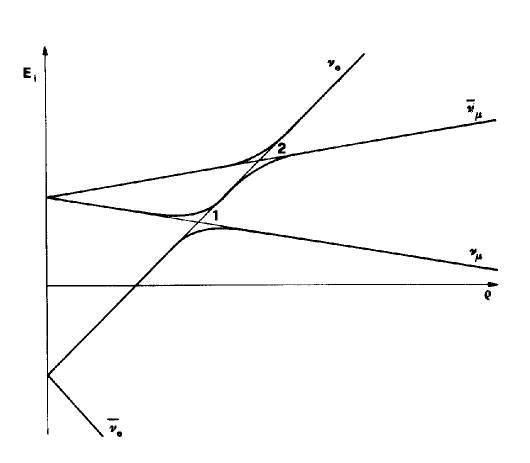
Figure 1: Neutrino energy levels vs matter density $\rho$ for the Majorana ($\nu_{e},\nu_{\mu}$) system with mixing and transition magnetic moment. 1 – MSW resonance, 2 – RSFP resonance.

There are two avoided level crossings now, i.e. two resonances. The resonance of the SFP occurs at higher densities than the MSW resonance. This can be easily understood if we compare the resonance conditions (12) and (13). Therefore a $\nu_{eL}$ born in the core of the sun and propagating outwards will first encounter the RSFP resonance and then the MSW one. However, if the adiabaticity condition of the RSFP is satisfied, the $\nu_{eL}$ will be adiabatically converted into the $\bar{\nu}_{\mu R}$ and so will never reach the MSW resonance. Thus, the MSW effect would be inoperative in this case, no matter how large the MSW adiabaticity parameter $\lambda_{\rm MSW}$.

The above situation refers to the case when the two resonances are well separated. If they overlap, an interesting interplay of the MSW effect and the RSFP of neutrinos may occur. The two resonances may either enhance or suppress each other, depending on their degree of adiabaticity. A detailed discussion of this interplay can be found in [18-21]. Another important consequence of the joint operation of the neutrino oscillations and SFP is the possibility of the transformation of the solar $\nu_{eL}$’s into $\bar{\nu}_{eR}$’s [7, 18, 22, 23, 24]. This may have very important experimental consequences which I will discuss later on.

4 Experimental data

I will now briefly discuss the available experimental data. At the moment we have the data from the five solar neutrino experiments: Homestake, GALLEX, SAGE, Kamiokande and Super–Kamiokande. All the data show some deficiency of the solar neutrinos, the degree of which varies from the experiment to the experiment. This was reviewed in the other talks at this conference [25, 26, 27]. I will concentrate on a different aspect of the data – their time structure. I will not discuss the Super–Kamiokande data since it is too early yet to discuss its possible time dependence.

As I have already mentioned, there are some indications of the time variations of the signal in the Homestake experiment. At the same time, the Kamiokande group did not observe any time variation of the solar neutrino signal in their experiment, which allowed them to put an upper limit on the possible time variation, $\Delta Q/Q<30\%$ at 90% c.l. [28]. The gallium experiments have not observed any statistically significant time variation of the signal either [27].

Some remarks about time structure of the Homestake data are in order. The data compare better with an assumption of a time–dependent signal than with that of a constant one, hinting to an anticorrelation with solar activity. For the solar cycles 20 and 21 the detection rate at the periods of the quiet sun exceeded that for the active sun by a factor of two or more. There are also some indications in favor of the semiannual variations, but their statistical significance is lower than that for the 11-year variations. There exist more than 20 analyses of the data which used a variety of statistical methods [29-53]. The authors of all these papers but three [30, 34, 51] came to the conclusion that the Homestake data (or at least part of it) shows a time variation in anticorrelation with solar activity. However, the obtained values of the correlation coefficients and the confidence level depend very much on the indicator of solar activity chosen, the statistical methods used and on the way the experimental errors are treated. Moreover, almost all the analyses were performed before 1990 and so did not take into account more recent runs (run 109 and later). These runs do not show a tendency to vary in time, similarly to the earlier runs 19–59. A recent analysis of Stanev [52] which updated the one of ref. [35] included the runs 109-133 and showed that this results in the correlation coefficient between the Homestake detection rate and the sunspot number being significantly decreased.

I would like to mention an interesting recent development in the analyses of the time structure of the Homestake data. Two groups [44, 46, 50] pointed out that the total sunspot number is too rough an indicator of solar activity which only characterizes its gross features. They argued than one should use a more local indicator if one is interested in the correlation with the solar neutrino signals. They suggested to use the direct measurements of the magnetic field strength on the surface of the sun along the line of the sight connecting the center of the sun and the earth, i.e. along the trajectory of the solar neutrinos observed at the earth [44, 46, 50]. The authors of these studies came to the conclusion that the (anti)correlation coefficient increases significantly if one uses this local characteristics of the solar activity. Another very interesting point was made by Massetti and Storini [53]. They found that the anticorrelation between the Homestake signal and the green corona line (which they chose as an estimator of the solar magnetic field) is much stronger for the neutrinos emitted in the southern solar hemisphere than for those emitted in the northern hemisphere. This conclusion was confirmed by Stanev [52]. This result may have a very interesting interpretation. As was reported by Rust at this conference [54], about 80% of the magnetic field ejected from the southern solar hemisphere has a right-handed twist ($\phi^{\prime}<0$), while about 80% of the field ejected from the northern hemisphere has a left-handed twist. As I mentioned before, the right-handed twist enhances the RSFP of neutrinos whereas the left-handed twist suppresses is. Therefore the observation of Massetti and Storini finds a very natural interpretation in the framework of the neutrino transition magnetic moment scenario (see [12, 13] for an early discussion of possible north-south effects due to the twisting magnetic fields). There is one more observation that supports this interpretation. As was noticed by Stanev [52], two solar cycles ago there was no significant time variation in the Homestake data (runs 19–59), similar to what was observed in 1990–1996. This may indicate that the Homestake data has a better 22-year periodicity than the 11-year one. Since the magnitude of the solar magnetic field changes with the 11-year periodicity whereas its $direction$ (including the twist) changes with the 22-year periodicity, this might be an additional argument for the RSFP in twisting magnetic fields as the solution of the solar neutrino problem.

The question of whether or not any time variations have been observed by the Homestake experiment is rather controversial. Unfortunately, the statistics of the Homestake experiment is poor and it is very difficult (if possible at all) to draw any definitive conclusion regarding the time dependence of the data. However, in any case the following question naturally arises: Can one reconcile, at least in principle, a strong time variation in the Homestake data with no observable time variation in Kamiokande and GALLEX experiments? I will show now that the answer to this question is yes, at least within the RSFP scenario. The RSFP mechanism can very naturally account for all the available solar neutrino data. Let me now briefly describe how this works.

5 Reconciling the time structure of the data

Suppose that we believe in strong (by a factor of two or more) time variations in the Homestake data. If we are to describe the absence of the observable time variations in the Kamiokande and gallium experiments, the mechanism responsible for the time variations must be neutrino energy dependent, otherwise the degree of the time variations in all these experiments would be the same. This excludes the ordinary neutrino spin precession which in energy independent. By contrast, the RSFP mechanism $is$ energy dependent, so it has at least a potential of accounting for the data. We shall now see that how this potential is realized.

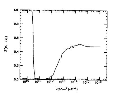
Figure 2: Typical RSFP “suppression pit”. This figure was borrowed from [58].

In many respects the RSFP of neutrinos is similar to the MSW effect. In particular, the $\nu_{eL}$ survival probability $P$ as the function of $E/\Delta m^{2}$ which determines the energy dependence of the effect is given by a “suppression pit”. A typical RSFP suppression pit is shown in Fig. 2. Its shape is similar to the MSW suppression pit, although there are some differences. For example, in the case of the MSW effect the r.h.s edge of the curve approaches unity, whereas for the RSFP it approaches 1/2. It has been emphasized in [55] that the RSFP–type shape of the suppression pit can explain very naturally the observed average depletions of the solar neutrino signal observed in different experiments (even if one forgets about any time variations): the low-energy $pp$ neutrinos are unsuppressed ($P\approx 1$ at the l.h.s. edge of the curve), the intermediate energy ⁷Be and ⁸B neutrinos are at the bottom of the suppression pit and so are strongly suppressed, whereas the high-energy part of the ⁸B neutrino spectrum is on the r.h.s. edge of the pit and therefore is suppressed by a factor of two. This is exactly what one needs to account for the experimental data. Notice that the same can be achieved in the case of the MSW effect by a rather fine adjustment of the $\Delta m^{2}$ parameter in order to place the high energy part of the ⁸B neutrino spectrum on the r.h.s. slope of the MSW suppression pit in such a way as to achieve a factor of two suppression on the average. In the case of the RSFP mechanism this comes out quite naturally and for a wider range of the values of the $\Delta m^{2}$ parameter.

5.1 GALLEX and SAGE

Let us see now discuss how the RSFP mechanism explains the lack of the time dependence of the signal in the gallium experiments.

The shape of the suppression pit depends on the profile and strength of the magnetic field of the sun. In particular, the depth of the pit depends on the maximum field strength while its width depends on the extension of solar magnetic field. Low energy neutrinos experience the RSFP conversion at high densities since the resonance density is inversely proportional to the neutrino energy [see eq. (12)]. Therefore they are sensitive to the magnetic field strength in the core of the sun. If such an inner magnetic field is absent or weak, the RSFP will not be effective for the low energy neutrinos and their survival probability will be close to unity. For this reason the position of the l.h.s. edge of the suppression pit in Fig. 2 (low–energy edge) depends on the strength of the inner magnetic field of the sun. We do not know if a strong magnetic field exists in the core of the sun; however, it is known that in any case, if exists, it must be practically constant in time.

Before the data of GALLEX and SAGE became available, one could had asked the following question: If one believes in the time variations in the Homestake data, can one predict the time structure of the signal in the gallium solar neutrino experiments? Riccardo Barbieri repeatedly asked me this question when I visited Pisa in 1989. The answer was given in [56]. This answer was conditional, depending on the average suppression of the signal, which, of course, was unknown at that time: If the average suppression of the signal is strong, there should be significant time variations of the signal, while if the average suppression is not too strong, no appreciable time variations should be detected. The reason for that is very simple. The inner magnetic field is unknown but in any case does not vary in time. If it is very strong, it may result in a significant (constant in time) suppression of the low-energy $pp$ neutrinos. In this case the time variations of the ⁸B neutrino contribution would be visible. On the other hand, if the inner magnetic field is weak, the $pp$ neutrino flux will leave the sun unscathed and constitute the major part of the signal. In this case even a strong time variation of the ⁸B neutrino flux will hardly be detectable since these neutrinos would constitute only a small fraction of the signal. We see now that this prediction is fully consistent with the results of GALLEX and SAGE. They imply that the $pp$ neutrino flux is unsuppressed; therefore within the RSFP scenario one should not see any appreciable time variations. As a matter of fact, no statistically significant time variations of the signal were observed. Thus, the results of the GALLEX and SAGE experiments can be easily fitted within the RSFP mechanism provided that the magnetic field in the core of the sun $B_{i}$ is not too strong. One can turn the argument around and ask the following question: If we believe in the RSFP mechanism, what is the maximum allowed inner magnetic field which is not in conflict with the gallium experiments? The answer turns out to be $(B_{i})_{max}\approx 3\times 10^{6}$ G assuming the neutrino transition magnetic moment $\mu=10^{-11}\mu_{B}$ [57].

5.2 Kamiokande

The question I am going to address now is how to reconcile strong time dependence of the signal in the Homestake experiment with no or little time variation of the Kamiokande data. I will show that this comes out quite naturally in the RSFP scenario. The key points here are that [56-59]

(1) The two experiments are sensitive to slightly different parts of the solar neutrino spectrum: Homestake is sensitive to the energetic ⁸B neutrinos as well as to medium–energy ⁷Be and $pep$ neutrinos, whereas the Kamiokande experiment is only sensitive to the high–energy part of ⁸B neutrinos ($E>7.5$ MeV);

(2) For Majorana neutrinos, the RSFP converts left-handed $\nu_{e}$ into right-handed $\bar{\nu}_{\mu}$ (or $\bar{\nu}_{\tau}$) which are sterile for the Homestake experiment (since their energy is less than the muon or tauon mass) but do contribute to the event rate in the Kamiokande experiment through their neutral–current interaction with electrons. Although the $\bar{\nu}_{\mu}e$ cross section is smaller than the $\nu_{e}e$ one, it is non-negligible, which reduces the amplitude of the time variation of the signal in the Kamiokande experiment. It turns out that the above two points are enough to account for the differences in the time dependences of the signals in the Homestake and Kamiokande experiments.

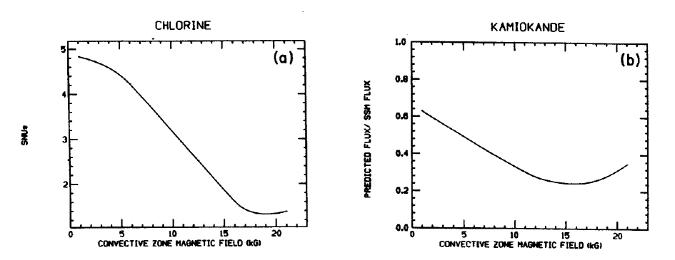
Figure 3: The calculated Homestake and Kamiokande detection rates vs convective zone magnetic field strength [58]. The neutrino transition magnetic moment $\mu=2\times 10^{-11}\mu_{B}$ is assumed.

In Fig. 3 are shown the event rates in the Homestake and Kamiokande experiments as functions of the convective zone magnetic field strength calculated by Babu, Mohapatra and Rothstein [58]. There are three important observations to be made. First, both rates decrease with magnetic field until they reach their minima, and then start to increase. Second, the minimum of the Kamiokande signal is situated at a lower magnetic field strength then the one of the Homestake signal. Third, the Kamiokande curve is less steep than the Homestake one. Let me explain this behavior of the curves. The third of the above observations obviously follows from the above point (2). For weak fields, the efficiency of the RSFP increases with the field (so that the counting rates decrease) because the adiabaticity of the transition improves. The situation changes, however, after the field becomes strong enough. As I discussed above, a $\nu_{eL}$ can be fully converted into the $\bar{\nu}_{\mu R}$ if it is born at a density much above the resonance one and passes through the RSFP resonance adiabatically. However, if it is born close to the resonance, the efficiency of the conversion decreases; for example, for the $\nu_{eL}$ born exactly at the resonance point, the conversion probability is only 1/2 even in the case of a perfectly adiabatic conversion. The resonance width $\Delta r$ is

$$\Delta r=\frac{2\mu B_{\bot r}}{\Delta m^{2}/2E}\,L_{\rm eff}\,,$$ (17)

so it increases with the field strength. For very strong magnetic fields the resonance becomes very wide, so the neutrino birth place becomes too close to the resonance region and the efficiency of the conversion decreases. This explains the existence of the minima of the detection rates in Fig. 3. From the above arguments it follows that there is an optimum value (or a range of values) of the resonance widths $\Delta r\simeq const$ which corresponds to the maximum efficiency of the RSFP, i.e. to the minima of the detection rates. Since $\Delta r\propto B_{\bot}E$, the higher the neutrino energy, the smaller the magnetic field strength at the minimum of the detection rate. This explains why the detection rate for the the Kamiokande experiment (which is sensitive to more energetic neutrinos) has its minimum situated at a lower magnetic field strength than that for the Homestake experiment.

Now let us look again at Fig. 3. Assume that during the solar cycle the convective field magnetic field changes, say, between 10 and 20 kG. For this range of $B_{c}$ the Homestake detection rate changes steeply. At the same time, the Kamiokande rate is close to its minimum and so varies very little. It is for this reason that the time variation of the Kamiokande signal may be much smaller than that of the Homestake signal. One can draw another important conclusion from the above discussion: The time structure of the Kamiokande (and now Super–Kamiokande) experiment may be more complicated than a mere anticorrelation with the solar activity. In particular, one can expect an anticorrelation during a part of the solar cycle and direct correlation during another part. This can be tested in the Super–Kamiokande experiment.

6 Fitting the data

I will now discuss more quantitatively how one fits the data. The main problem one encounters is that the magnetic field inside the sun is practically unknown. In the case of the MSW effect, all the experimental data are analyzed in terms of the two unknown parameters: $\Delta m^{2}$ and $\sin^{2}2\theta_{0}$. In the case of the RSFP mechanism the situation is much more complicated. One has an unknown parameter $\Delta m^{2}$ and an unknown function – magnetic field profile in the sun $B_{\bot}(r)$ (in fact, there is one more parameter – the neutrino transition magnetic moment, but it enters the problem only through the product $\mu B_{\bot}$). In such a situation the only thing one can do is to try various “plausible” magnetic field configurations, calculate the detection rates for various solar neutrino experiments and compare them with the experimental results. Such a program was carried out in a number of papers (see, e.g., [15-22, 55, 57-64]). I will discuss briefly the results of the two recent papers [57, 64]. In [57] nine different model magnetic field profiles were used. The neutrino mass mixing was assumed to be absent. Two of the nine magnetic field profiles used reproduced the data very well, while the others either produced poor quality fits or completely failed to reproduce the data. This shows that one can in principle discriminate between various models of the solar magnetic field using the solar neutrino data. The upper limit on the inner magnetic field which I already mentioned before was established. The typical values of the parameters that produced the good fits of the data were $\Delta m^{2}\simeq(4\times 10^{-9}-2\times 10^{-8})$ eV², with the maximum magnetic field strength varying between $\simeq 25$ and $\simeq 50$ kG during the solar cycle (assuming $\mu=10^{-11}\mu_{B}$).

In [64] it was assumed that the neutrino mass mixing is present ($\theta_{0}\neq 0$) i.e. the combined effect of the RSFP and neutrino oscillations was studied. The neutrino signals in the chlorine, gallium and Kamiokande experiments were calculated using nine different model magnetic field profiles. Three of the nine magnetic field configurations used produced good fits of all the data. Typical values of the neutrino parameters required to account for the data are $\Delta m^{2}\simeq(10^{-8}$–$10^{-7})$ eV², $\sin 2\theta_{0}\buildrel<\over{{}_{\sim}}$ 0.25; larger mixing angles are excluded by the GALLEX and SAGE data. For neutrino transition magnetic moment $\mu=10^{-11}\mu_{B}$ the maximum magnetic field in the solar convective zone has to vary in time in the range (15–30) kG.

As I have already mentioned, if neutrinos experience the RSFP in the sun and also have mass mixing, a flux of electron antineutrinos can be produced. This flux is in principle detectable in the SNO, Super–Kamiokande and Borexino experiments even in the case of moderate neutrino mixing angles [7, 18, 22, 23, 24]. The main mechanism of the $\bar{\nu}_{eR}$ production is $\nu_{eL}\rightarrow\bar{\nu}_{\mu R}\rightarrow\bar{\nu}_{eR}$, where the first transition is due to the RSFP in the sun and the second one is due to the vacuum oscillations of antineutrinos on their way between the sun and the earth. The salient feature of this flux is that it should vary in time in anticorrelation with the variation of the $\nu_{eL}$ flux. The detection of the solar $\bar{\nu}_{eR}$ flux would be a signature of the combined effect of the RSFP and neutrino oscillations. It could allow one to discriminate between small mixing angle ($\sin 2\theta_{0}\buildrel<\over{{}_{\sim}}0.1$) and moderate mixing angle ($\sin 2\theta_{0}\simeq 0.1-0.25$) solutions. For the mixing angles $\sin 2\theta_{0}\buildrel>\over{{}_{\sim}}0.3$, a large flux of electron antineutrinos would be produced in contradiction with an upper limit already derived from the Kamiokande and LSD data [65, 66].

The $\bar{\nu}_{eR}$ flux can be significantly enhanced if the solar magnetic field changes its direction along the neutrino trajectory, i.e. twists [14, 17]. In this case one can have a detectable $\bar{\nu}_{eR}$ flux even if the neutrino magnetic moment is too small or the solar magnetic field is too weak to account for the solar neutrino problem [17].

7 Predictions for future experiments

The predictions of the RSFP mechanism for the Super–Kamiokande experiment are very similar to the ones for Kamiokande: as I discussed above, one can expect small time variations, not necessarily in anticorrelation with the solar activity. In fact, during a part of the solar cycle the signal may vary in direct correlation with the solar magnetic field. Similar prediction is made for the charged–current (CC) signal in SNO. However, in that case one should expect somewhat stronger time variations since the $\bar{\nu}_{\mu R}$ or $\bar{\nu}_{\tau R}$ produced as a result of the RSFP do not contribute to the CC signal. The neutral–current signal in SNO should remain constant in time (unless neutrinos precess into sterile states, i.e. are Dirac particles) modulo the trivial 7% seasonal variations of the signal because of the varying distance between the sun and the earth. This along with the varying CC signal would be a clear signature of the neutrino spin-flavor precession.

The ⁷Be neutrino flux is expected to be strongly suppressed; it should also vary in time, which may in principle be observable in the Borexino experiment. The expected variation of the ⁷Be neutrino flux is about 30% (40%) for $\sin 2\theta_{0}\simeq 0.24$ (0) [64].

For not too small neutrino mass mixing $(\sin 2\theta_{0}\buildrel>\over{{}_{\sim}}0.1)$, one can also expect a flux of the $\bar{\nu}_{eR}$ coming from the sun, with a distinct feature of time variation in an anti-phase with the solar $\nu_{eL}$ flux. Such a flux may be observable in the SNO, Super–Kamiokande and Borexino experiments [64].

Even though the predicted time variation for Super–Kamiokande (and to some extent also for SNO) are smaller than the variations in the Homestake experiments, its amplitude cannot be smaller than 10–15% provided that one believes in the time variations of the Homestake signal by a factor of two or more. Such a variation should be clearly detectable in the Super–Kamiokande. The amplitude of time variation of the charged-current signal in SNO should be even larger.

Thus, the RSFP mechanism leads to very distinct and testable predictions.

8 Pro et Contra

I will summarize now the arguments for and against the RSFP mechanism as the solution of the solar neutrino problem and comment on them. I start with the objections to this mechanism that are frequently put forward.

$\bullet$ There isn’t any time variation in the Homestake data; therefore there is nothing to discuss.

I will not comment on this point.

$\bullet$ There is no compelling evidence for time variation of the Homestake signal; the errors are too large to draw any definitive conclusions.

This is certainly correct. Fortunately, the Super–Kamiokande has (and SNO is expected to have) a much higher detection rate than all the previous experiments; therefore one can hope that the question of whether or not the observed solar neutrino signal varies in time will be settled in a few years.

$\bullet$ Kamiokande has not observed any time variation of the signal during more than eight years of data taking; this disproves transition magnetic moment scenario.

This conclusion is just wrong, as I explained in detail above.

$\bullet$ GALLEX and SAGE have not observed any time variation of the signal. Moreover, these experiments did not detect strong suppression of the signal during the period of high solar activity, which contradicts the transition magnetic moment scenario.

This is also wrong and was also discussed above.

$\bullet$ Neutrino magnetic moments are severely constrained from above by astrophysics data; solar magnetic field is not strong enough to produce any sizeable spin or spin–flavor precession.

For the maximum magnetic field of the sun of the order of a few tens kG the requisite value of the neutrino transition magnetic moment $\mu\simeq 10^{-11}\mu_{B}$. This is consistent with the existing laboratory upper bounds on $\mu$ and also with the astrophysics bounds coming from the white dwarf cooling rates. There are also a factor of 3 to 10 more stringent bounds coming from the cooling rates of the helium stars. However, at this level the bounds become less reliable. In any case, a factor of ten smaller $\mu$ would require a factor of ten stronger magnetic fields for the RSFP to proceed with the same efficiency. There are even more stringent bounds on neutrino magnetic moments coming from the neutrino signal observations from the supernova 1987A. However, these bounds are not applicable to the transition magnetic moments of Majorana neutrinos. The reason is very simple: These bounds are based on the assumption that neutrinos can be converted into right-handed sterile states in the supernova because of scattering on the particles of the matter through the photon exchange. Sterile neutrinos then escape freely from the dense core of the supernova instead of being trapped. However, in the case of Majorana neutrinos the resulting right-handed states are right-handed antineutrinos which are not sterile and therefore are still trapped.

The second part of the above objection, as well as next two, concerns the solar magnetic field. I will comment on them altogether.

$\bullet$ Solar magnetic field is only strong in sunspots which occupy a small part of the solar surface; there is no strong enough large-scale magnetic field in the sun.

$\bullet$ The equatorial gap in the toroidal magnetic field of the sun is rather wide, so that the year-averaged field affecting the solar neutrinos should be small.

Unfortunately, the magnetic field inside the sun is not accessible to direct observations and is very poorly known. At the moment, there is no compelling model of the solar magnetic field (in particular, there is no model capable of predicting the 11-year period of the solar cycle). Probably, this is related to the fact that the magnetic field plays a relatively minor role in the solar dynamics. The sole robust upper limit on the strength of the solar magnetic field comes from the requirement that the field pressure be smaller than the matter pressure; this is a rather weak limit (for the convective zone, $B\buildrel<\over{{}_{\sim}}10^{7}$ G). There are more stringent bounds, but they are highly model dependent. Regarding the equatorial gap in the toroidal magnetic field of the sun. It is not very well defined; there are even periods when groups of the sunspots cross the solar equator. In any case, even if such a gap exist on the solar surface, it is not clear if it exists, e.g., near the bottom of the convective zone. To summarize, I think it is fair to say that at the moment there is a better chance to learn something about the solar magnetic field by studying the solar neutrinos than vice versa.

$\bullet$ It is difficult to construct a particle-physics model which would naturally produce large enough magnetic moments while keeping neutrino mass small.

This is correct, such models are not easy to construct. In the standard model of electroweak interactions the magnetic moment of electron neutrino is $\mu_{\nu_{e}}\approx 3\times 10^{-19}\mu_{B}\,(m_{\nu_{e}}/{\rm eV})$, far too small to be of relevance for the solar neutrino problem. It is not difficult to construct an extension of the standard model with large enough $\mu_{\nu_{e}}$ or transition moment $\mu$; what is really difficult is to keep the neutrino mass naturally small in such a model. By “naturally” I mean to have neutrino mass small without introducing additional fine tuning of the parameters in the model.

The standard electroweak model is full of fine-tuning, or hierarchy, problems (for example, why is $m_{e}$ more than 5 orders of magnitude smaller than the top quark mass?), so one could take an attitude that all these hierarchy problems will one day be solved altogether by a more general model which will encompass the standard electroweak model. However, it would be good to avoid introducing new fine tuning problems in the model if it is possible. Interestingly, there exist several successful attempts to construct such models, some of them very appealing (see, e.g., [67, 68]). Most of these models use various versions of the so-called Voloshin’s symmetry [69] to keep neutrino mass small without invoking a fine tuning.

Now about the arguments supporting the RSFP scenario. I will mention only one of them: The RSFP mechanism is fully consistent with all the currently available solar neutrino data.

Let me conclude with two remarks. Both neutrino oscillations and spin (or spin–flavor) precession require some extension of the standard model of the electroweak interactions: in the minimal standard model neutrinos are massless and have zero magnetic moments. The most popular models of the neutrino mass invoke the so-called see-saw mechanism which requires some new physics at a very high energy scale, typically at the GUT scale $\sim 10^{16}$ GeV or “intermediate” scale $\sim 10^{12}$ GeV. Obviously, this new physics cannot be directly probed. On the other hand, all the extensions of the standard electroweak model which are capable of producing $\mu_{\nu}\sim(10^{-12}-10^{-11})\mu_{B}$ require some new physics at the energy scale $\sim$ a few hundreds GeV, i.e. close to the electroweak scale. This physics will hopefully become accessible to direct experimental tests in the near future.

In the beginning of the solar neutrino studies, when the first experiment was discussed and planned, the main idea was to probe the sun using the neutrinos it emits as a tool. Neutrinos themselves were considered standard and very well understood. Now the situation is quite different. It seems that now we know much more about the sun than we know about the neutrinos, so we can use the sun as a unique laboratory to study the neutrinos. In doing so, we should explore the neutrino properties in a broadest possible way, trying to get as much as possible information about all the neutrino characteristics that can be probed. The neutrino magnetic moment is one of them.

References

- [1] J.N. Bahcall, M.H. Pinsonneault, S. Basu, J. Cristensen-Dalsgaard, Phys. Rev. Lett. 78 (1997) 171.
- [2] See, e.g., S.T. Petcov, these Proceedings; N. Hata, P. Langacker, hep-ph/9705339.
- [3] A. Cisneros, Astrophys. Space Sci. 10 (1970) 87.
- [4] M.B. Voloshin, M.I. Vysotsky, Sov. J. Nucl. Phys. 44 (1986) 845; M.B. Voloshin, M.I. Vysotsky, L.B. Okun, Sov. Phys. JETP 64 (1986) 446.
- [5] R. Barbieri, G. Fiorentini, Nucl. Phys. B304 (1988) 909.
- [6] J. Schechter, J.W.F. Valle, Phys. Rev.D24 (1981) 1883; ibid.D25 (1982) 283 (E).
- [7] C.-S. Lim, W.J. Marciano, Phys. Rev. D37 (1988) 1368.
- [8] E.Kh. Akhmedov, Sov. J. Nucl. Phys. 48 (1988) 382; Phys. Lett. B213 (1988) 64.
- [9] S.P. Mikheyev, A.Yu. Smirnov, Sov. J. Nucl. Phys. 42 (1985) 913.
- [10] L. Wolfenstein, Phys. Rev. D17 (1978) 2369.
- [11] C. Aneziris, J. Schechter, Int. J. Mod. Phys. A6 (1991) 2375; Phys. Rev. D45 (1992) 1053.
- [12] A.Yu. Smirnov, Phys. Lett. B260 (1991) 161.
- [13] E.Kh. Akhmedov, P.I. Krastev, A.Yu. Smirnov, Z. Phys. C52 (1991) 701.
- [14] E.Kh. Akhmedov, S.T. Petcov, A.Yu. Smirnov, Phys. Rev. D48 (1993) 2167; Phys. Lett. B309 (1993) 95.
- [15] T. Kubota, T. Kurimoto, M. Ogura, E. Takasugi, Phys. Lett. B292 (1992) 195; T. Kubota, T. Kurimoto, E. Takasugi, Phys. Rev. D49 (1994) 2462.
- [16] P.I. Krastev, Phys. Lett. B303 (1993) 75.
- [17] A.B. Balantekin, F. Loreti, Phys. Rev. D48 (1993) 5496.
- [18] E.Kh. Akhmedov, Sov. Phys. JETP 68, 690 (1989).
- [19] E.Kh. Akhmedov, Phys. Lett. B257 (1991) 163.
- [20] H. Minakata, H. Nunokawa, Phys. Rev. Lett. 63 (1989) 121.
- [21] A.B. Balantekin, P.J. Hatchell, F. Loreti, Phys. Rev. D41 (1990) 3583.
- [22] E.Kh. Akhmedov, Phys. Lett. B255 (1991) 84.
- [23] R.S. Raghavan et al., Phys. Rev. D44 (1991) 3786.
- [24] A.B. Balantekin, F. Loreti, Phys. Rev. D45 (1992) 1059.
- [25] K. Lande, these Proceedings.
- [26] Y. Suzuki, these Proceedings.
- [27] T. Kirsten, these Proceedings; T. Bowles, these Proceedings.
- [28] A. Suzuki, In Proc. of the 7th Int. Workshop on Neutrino Telescopes, Venezia, February 24 – March 1, 1996. M. Baldo Ceolin (Ed.), p. 263.
- [29] W.R. Sheldon, Nature 221 (1969) 650.
- [30] L.J. Lanzaretti, R.S. Raghavan, Nature 293 (1981) 122.
- [31] G.A. Bazilevskaya, Yu.I. Stozhkov, T.N. Charakhchyan, Sov. Phys. JETP Lett. 35 (1982) 341.
- [32] V.N. Gavrin, Yu.S. Kopysov, N.T. Makeev, JETP Lett. 35 (1982) 608.
- [33] J.N. Bahcall, G.B. Field, W.H. Press, Astroph. J. 320 (1987) L69.
- [34] R.M. Wilson, Solar Phys. 112 (1987) 1.
- [35] J.W. Bieber, D. Seckel, T. Stanev, G. Steigman, Nature 348 (1990) 407.
- [36] L.M. Krauss, Nature 348 (1990) 403.
- [37] B.W. Filippone, P. Vogel, Phys. Lett. B246 (1990) 546.
- [38] J.N. Bahcall, W.H. Press, Astroph. J. 370 (1991) 730.
- [39] G. Fiorentini, G. Mezzorani, Phys. Lett. B253 (1991) 181.
- [40] H. Nunokawa, H. Minakata, Int. J. Mod. Phys. A6 (1991) 2347.
- [41] V. Gavryusev, E. Gavryuseva, A. Roslyakov, Sol. Phys. 133 (1991) 161.
- [42] Ph. Delache et al., Astrophys. J. 407 (1993) 801.
- [43] X. Shi et al., Comm. Nucl. Part. Phys. 21 (1993) 151.
- [44] D.S. Oakley et al., Astrophys. J. 437 (1994) L63.
- [45] R.L. McNutt Jr, Science 270 (1995) 1635.
- [46] V.N. Obridko, Yu. R. Rivin, Izv. RAN, ser. fiz., No 9, (1995).
- [47] S. Massetti M. Storini, N. Iucci, Proc. 24th ICRC (Rome), 4, 1243 (1995).
- [48] S. Massetti, M. Storini, J. Sýkora, Proc. 24th ICRC (Rome), 4, 1247 (1995).
- [49] L.I. Dorman, V.L. Dorman, A.W. Wolfendale, Proc. 24th ICRC (Rome),4, (1995).
- [50] D.S. Oakley, B. Herschel, hep-ph/9604252.
- [51] M. Lissia, In Proc. 4th Intern. Topical Workshop “New Trends in Solar Neutrino Physics, V. Berezinsky and G. Fiorentini (eds.), Gran Sasso, Italy, 1996, p. 129.
- [52] T. Stanev, In Proc. 4th Intern. Topical Workshop “New Trends in Solar Neutrino Physics, V. Berezinsky and G. Fiorentini (eds.), Gran Sasso, Italy, 1996, p. 141.
- [53] S. Massetti, M. Storini, Astrophys, J. 472 (1996) 827.
- [54] D. Rust, these Proceedings.
- [55] C.S. Lim, H. Nunokawa, Astropart. Phys. 4 (1995) 63.
- [56] E.Kh. Akhmedov, KIAE preprint IAE-5017/1, 1990 (unpublished). A very short version of this work was published in Nucl. Phys. A527 (1991) 679c.
- [57] E.Kh. Akhmedov, A. Lanza, S.T. Petcov, Phys Lett. B303 (1993) 85.
- [58] K.S. Babu, R.N. Mohapatra, I.Z. Rothstein, Phys. Rev. D44 (1991) 2265.
- [59] Y. Ono, D. Suematsu, Phys. Lett. B271 (1991) 165.
- [60] E.Kh. Akhmedov, O.V. Bychuk, Sov. Phys. JETP 68 (1989) 250.
- [61] P.I. Krastev, A.Yu. Smirnov, Z. Phys. C49 (1991) 675.
- [62] H. Minakata, H. Nunokawa, Phys. Lett. B314 (1993) 371.
- [63] J. Pulido, Phys. Rev. D48 (1993) 1492
- [64] E.Kh. Akhmedov, A. Lanza, S.T. Petcov, Phys. Lett. B348 (1995) 124.
- [65] R. Barbieri et al., Phys. Lett. B 259, 119 (1991).
- [66] LSD Collaboration, M. Aglietta et al., preprint ICGF 269/92.
- [67] K.S. Babu, R.N. Mohapatra, Phys. Rev. Lett. 63 (1989) 228.
- [68] S.M. Barr, E.M. Freire, A. Zee, Phys. Rev. Lett. 65 (1990) 2626.
- [69] M.B. Voloshin, Sov. J. Nucl. Phys.48 (1988) 512.