Lepton flavour violation in a left-right symmetric model

Abstract:

We consider in this paper a Left-Right symmetric gauge model in which a global lepton-number-like symmetry is introduced and broken spontaneously at a scale $\omega$ that could be as low as $10^{4}$ GeV or so. The corresponding physical Nambu-Goldstone boson, which we call majoron and denote $J$, can have tree-level flavour-violating couplings to the charged fermions, leading to sizeable majoron-emitting lepton-flavour-violating weak decays. We consider explicitly a leptonic variant of the model and show that the branching ratios for $\mu\to e+J$, $\tau\to e+J$ and $\tau\to\mu+J$ decays can be large enough to fall within the sensitivities of future $\mu$ and $\tau$ factories. On the other hand the left-right gauge symmetry breaking scale may be as low as few TeV.

1 Introduction

Apart from offering a possibility of understanding parity violation on the same footing as gauge symmetry breaking, left-right symmetric extensions of the standard electroweak theory naturally incorporate small neutrino masses [1, 2]. Unfortunately, for phenomenologically interesting values of the scale at which the $SU(2)_{R}$ symmetry gets broken ($\;<$$\sim\;$ 10 TeV) one expects the neutrino masses to lie close to their present laboratory limits, unless the neutrino Yukawa couplings are suppressed.

It is well known that, if stable, neutrinos would contribute too much to the energy density of the universe if their mass exceeds 60 eV or so [3]. Thus heavy neutrinos can be consistent with cosmology only if there are new neutrino decay and/or annihilation channels in addition to those induced by the standard model interactions.

The most attractive possibility to provide such new interactions is realized in models where the neutrino mass arises from the spontaneous violation of a global $B-L$ symmetry [4]. In this case there are invisible neutrino decays by majoron emission which can reconcile the large neutrino masses with cosmological density arguments [5, 6, 7]. Moreover, the new majoron decay and/or annihilation channels may also make these model consistent with cosmological Big-Bang nucleosynthesis [8, 9], while avoiding conflict with astrophysics [10].

Unfortunately, since $B-L$ is a gauge symmetry, its spontaneous breaking in the left-right symmetric framework does not imply the existence of a majoron and, as a result, the possibility of fast neutrino decay and/or annihilations is absent. Consequently, neutrino masses and the scale of left-right symmetry breaking are strongly restricted.

In order to cope with this problem a variant of the left-right symmetric model with an additional spontaneously broken U(1) global symmetry was proposed in ref. [11]. In order to implement such symmetry one adds new $SU(2)_{L}$ singlet leptons on which it acts nontrivially. These isosinglet leptons mix with the ordinary neutrinos and are involved in generating their mass. As a result, though the U(1) global symmetry differs from the usual $B-L$ symmetry, it plays an important role in generating the neutrino masses and decays. Extending the majoron concept to cover this situation, we still call majoron the Nambu-Goldstone boson that follows from the breaking of the U(1) global symmetry. It has been shown in ref. [11] that majoron-emitting neutrino decays e.g. $\nu_{\tau}$ $\rightarrow\nu+J$ can easily reconcile the large neutrino masses and the low left-right symmetry breaking scales with the cosmological restrictions.

In this paper we extend this class of models also in the charged fermion sector by adding electrically charged $SU(2)_{L}$ singlets. These have been widely discussed in the case of baryon-number and lepton-number-carrying SU(2) singlets, so-called lepto-quarks, both in the context of superstring inspired models [12] or simply added to the electroweak theory directly [13, 14]. Models with vector-like isosinglet quarks and leptons have also been invoked in the context of models with universal seesaw mechanism to explain the fermion masses [15]. On the other hand their phenomenological implications as well as the prospects for searching at high energy colliders have also been the subject of dedicated experimental study groups. In the present paper we consider, for simplicity the case of leptons in detail. This extension can have interesting phenomenological implications. We pay special attention to the flavour non–diagonal majoron couplings to usual charged leptons, electron, muon and tau. These would lead to the existence of majoron-emitting lepton-flavour-violating weak decays,

$$\mu\to e+J\qquad\tau\to e+J\qquad\tau\to\mu+J$$ (1)

(here $J$ denotes the majoron which follows from the spontaneous violation of the U(1) symmetry). Such decays have already been considered in other contexts, see e.g. ref. [16]. They would lead to bumps in the final lepton energy spectrum, at half of the parent lepton mass. These decays have been searched for experimentally [17, 18] but the limits on their possible existence are still rather poor, especially for the case of taus.

Restricting ourselves to the case where the global symmetry breaking scale is the largest, we derive analytically by two alternative methods, the direct one and the Noether current method of ref. [19], the general structure of the couplings of the charged leptons to the majoron, focusing on the off-diagonal couplings that lead to the decays above. We also consider the more general case where the hierarchy of scales is relaxed. Our numerical calculations show that these decays may have branching ratios which fall within the sensitivities of future $\mu$ and $\tau$ factories [20, 21].

2 The Model

We consider a model based on the gauge group

$$G_{LR}\equiv SU(2)_{L}\otimes SU(2)_{R}\otimes U(1)_{B-L}$$

in which an extra $U(1)_{G}$ global symmetry is postulated. In addition to the conventional quarks and leptons, there is a neutral gauge singlet fermion . These extra electrically neutral leptons might arise in superstring models [22]. They have also been discussed in an early paper of Wyler and Wolfenstein [23]. We do not use the more conventional triplet higgs scalars, which are absent in many of these string models. Instead we will substitute them by the doublets $\chi_{L}$ and $\chi_{R}$.

	$SU(2)_{L}\;\otimes$	$SU(2)_{R}\;\otimes$	$U(1)_{B-L}\;\otimes$	$U(1)_{G}$
$Q_{Li}$	2	1	1/3	0
$Q_{Ri}$	1	2	1/3	0
$\psi_{Li}$	2	1	$-1$	0
$\psi_{Ri}$	1	2	$-1$	0
$E_{Li}$	1	1	$-2$	$-1$
$E_{Ri}$	1	1	$-2$	1
$S_{Li}$	1	1	0	1
$\phi$	2	2	0	0
$\chi_{L}$	2	1	$-1$	1
$\chi_{R}$	1	2	$-1$	$-1$
$\sigma$	1	1	0	2

Table 1: $SU(2)_{L}\otimes SU(2)_{R}\otimes U(1)_{B-L}\otimes U(1)_{G}$ assignments of the quarks, leptons and higgs scalars.

In addition to this fermion content which was discussed in the earlier model [11], we introduce one $SU(2)_{L}\otimes SU(2)_{R}$ singlet charge-$-1$ lepton $E_{i}$ for each generation. These carry $B-L$ of $-2$. The left-handed and right-handed components of $E_{i}$ carry the global $U(1)_{G}$ charges of $-1$ and $+1$ respectively. The matter and Higgs boson representation contents are specified in Table 1. With these assignments, the most general Yukawa interactions allowed by the $G_{LR}\otimes U(1)_{G}$ symmetry are given as

$$-{\cal L}_{Y}=g_{1}\bar{Q}_{L}\phi Q_{R}+g_{2}\bar{Q}_{L}\tilde{\phi}Q_{R}+g_{3}\bar{\psi}_{L}\,\phi\,\psi_{R}+g_{4}\bar{\psi}_{L}\tilde{\phi}\psi_{R}+g_{5}[\bar{\psi}_{L}\chi_{L}S^{c}_{R}+\bar{\psi}_{R}\chi_{R}S_{L}]$$

$$+g_{6}\bar{S}_{L}S^{c}_{R}\sigma+ig_{7}\left(\bar{\psi}_{L}\tau_{2}\chi_{L}^{*}E_{R}-\bar{E}_{L}\chi_{R}^{T}\tau_{2}\psi_{R}\right)+g_{8}\bar{E}_{L}E_{R}\sigma^{*}+h.c.$$ (2)

where $g_{i}$ are matrices in generation space and $\tilde{\phi}=\tau_{2}\phi^{*}\tau_{2}$ denotes the conjugate of $\phi$. This Lagrangian is invariant under parity operation $Q_{L}\leftrightarrow Q_{R}$, $\psi_{L}\leftrightarrow\psi_{R}$, $E_{L}\leftrightarrow E_{R}$, $S_{L}\leftrightarrow S^{c}_{R}$, $\phi\leftrightarrow\phi^{\dagger}$ and $\chi_{L}\leftrightarrow\chi_{R}$.

The symmetry breaking pattern is specified by the following scalar boson vacuum expectation values (VEVs), assumed real:

$$\left\langle\phi\right\rangle=\left(\begin{array}[]{cc}k&0\\ 0&k^{\prime}\end{array}\right)\>;\left\langle\chi_{L}\right\rangle=\left(\matrix{v_{L}\cr 0}\right)\>;\left\langle\chi_{R}\right\rangle=\left(\matrix{v_{R}\cr 0}\right)\>;\left\langle\tilde{\phi}\right\rangle=\left(\begin{array}[]{cc}k^{\prime}&0\\ 0&k\end{array}\right)\>;\left\langle\sigma\right\rangle=\omega$$ (3)

The spontaneous violation of the global $U(1)_{G}$ symmetry generates a physical majoron whose exact profile is specified as

$$\left(\omega^{2}+\frac{v_{L}^{2}v^{2}}{V^{2}r}\right)^{-\frac{1}{2}}\left\{\omega\sigma_{I}+\frac{1}{V^{2}v_{R}^{2}r}\Bigl{[}v_{R}^{2}v^{2}(v_{L}\chi_{L}^{I})-v_{L}^{2}v^{2}(v_{R}\chi_{R}^{I})-v_{L}^{2}v_{R}^{2}(k\phi_{2}-k^{\prime}\phi_{4})\Bigr{]}\right\}$$ (4)

where $\sigma_{I}$, $\chi_{L}^{I}$, $\chi_{R}^{I}$, $\phi_{2}$ and $\phi_{4}$ denote the imaginary parts of the neutral fields in $\sigma$, $\chi_{L}$, $\chi_{R}$ and the bidoublet $\phi$. Here we have also defined the VEVs as $v^{2}\equiv k^{2}+k^{\prime 2}$ and $V^{2}\equiv v^{2}+v_{L}^{2}$, and

$$r=1+\frac{v^{2}v_{L}^{2}}{V^{2}v_{R}^{2}}.$$ (5)

Clearly, as it must, the majoron is orthogonal to the Goldstone bosons eaten-up by the $Z$ and the new heavier neutral gauge boson $Z^{\prime}$ present in the model. The latter acquires mass at the larger scale $v_{R}$.

In the limit $V^{2}\ll\omega^{2}\ll v_{R}^{2}$, the majoron becomes

$$J=\left(\omega^{2}+\frac{v_{L}^{2}v^{2}}{V^{2}}\right)^{-\frac{1}{2}}\left\{\omega\sigma_{I}+\frac{v_{L}v}{V^{2}}\left[v\chi_{L}^{I}-\frac{v_{L}}{v}(k\phi_{2}-k^{\prime}\phi_{4})\right]\right\}$$ (6)

Note that in this limit, the majoron has no component along the imaginary part of $\chi_{R}$ despite the fact that $\chi_{R}$ is nontrivial under the global symmetry. This was the limit considered in [11].

Here, in order to determine analytically the light charged-lepton masses and majoron couplings, we will restrict ourselves to the case where $\omega$ is the largest scale. In the limit $V^{2}\ll v_{R}^{2}\ll\omega^{2}$, and $r\rightarrow 1$, the majoron field becomes

$$J=\left(\omega^{2}+\frac{v_{L}^{2}v^{2}}{V^{2}}\right)^{-\frac{1}{2}}\left\{\omega\sigma_{I}+\frac{1}{V^{2}}\Bigl{[}v^{2}(v_{L}\chi_{L}^{I})-\frac{v_{L}^{2}v^{2}}{v_{R}^{2}}(v_{R}\chi_{R}^{I})-v_{L}^{2}(k\phi_{2}-k^{\prime}\phi_{4})\Bigr{]}\right\}$$ (7)

The various scales appearing in eq. (7) are not arbitrary. First of all, note that the minimization of the scalar potential dictates the consistency relation [2]

$$\frac{v_{R}}{v}\sim\lambda\frac{\omega}{v_{L}}$$ (8)

For $\lambda\sim 1$ the singlet VEV is necessarily larger than $v_{L}$ i.e. $v_{L}\ll\omega$ and, as a result, the majoron is mostly singlet and the invisible decay of the $Z$ to the majoron is enormously suppressed, unlike in the purely doublet or triplet majoron schemes.

On the other hand, in order that majoron emission does not overcontribute to stellar energy loss one needs to require [24] in the general case

$$\frac{g_{eeJ}}{m_{e}}\raise 1.29167pt\hbox{$\;<$\kern-7.5pt\raise-4.73611pt\hbox{$\sim\;$}}10^{-9}~{}\mbox{GeV}^{-1}\;,$$ (9)

where $g_{eeJ}$ is the majoron diagonal coupling to electrons. In the limit $V^{2}\ll v_{R}^{2}\ll\omega^{2}$, and $r\rightarrow 1$, one needs to require (see eq. (24))

$$\frac{v_{L}^{2}}{\omega V^{2}}\raise 1.29167pt\hbox{$\;<$\kern-7.5pt\raise-4.73611pt\hbox{$\sim\;$}}10^{-9}~{}\mbox{GeV}^{-1}\;,$$ (10)

One sees that eq. (8) and eq. (10) allow for the existence of right-handed weak interactions at accessible levels, provided $v_{L}$ is sufficiently small.

The diagonal couplings of the majoron, for example to electrons, may also have important implications in cosmology and astrophysics [7].

3 Charged Lepton Masses

Once all gauge and global symmetries get broken, mass terms are generated for the charged leptons, which are given by

$$-{\cal L}_{mass}=\bar{l}_{L}(g_{3}k^{\prime}+g_{4}k)l_{R}-\bar{l}_{L}g_{7}v_{L}E_{R}-\bar{E}_{L}g_{7}v_{R}l_{R}+\bar{E}_{L}g_{8}\omega E_{R}+h.c.$$ (11)

It may be written in block form as

$$-{\cal L}_{mass}=\left(\begin{array}[]{cc}\bar{l}_{L}&\bar{E}_{L}\end{array}\right)M\left(\begin{array}[]{c}l_{R}\\ E_{R}\end{array}\right)+h.c.\qquad\quad M=\left(\begin{array}[]{c}\end{array}\begin{array}[]{cc}M_{D}&M_{L}\\ M_{R}&M_{S}\end{array}\right)\;,$$ (12)

where the various entries are specified as

$$M_{D}=g_{3}k^{\prime}+g_{4}k\,,\quad M_{L}=-g_{7}v_{L}\,\quad M_{R}=-g_{7}v_{R}\,,\quad M_{S}=g_{8}\omega.$$ (13)

Here the matrix $M_{D}$ is the Dirac mass term determined by the standard Higgs bi-doublet VEV $\left\langle\phi\right\rangle$ responsible for quark and charged lepton masses, $M_{L}$ and $M_{R}$ are $G$ and $B-L$ violating mass terms determined by $v_{L}$ and $v_{R}$, while $M_{S}$ is a gauge singlet $G$-violating mass, proportional to the VEV of the gauge singlet higgs scalar $\sigma$ carrying 2 units of $G$ charge.

In order to determine analytically the light charged-lepton masses and majoron couplings we will work in the seesaw approximation, which we define as $M_{S},M_{R}\gg M_{D},M_{L}$. In this case the mass matrix in eq. (12) can be brought to block diagonal form via a bi-unitary transformation with two unitary matrices $V_{L}$ and $V_{R}$. In the see-saw approximation, $V_{L}$ and $V_{R}$ can be written in the form:

$$V_{L}=\left(\begin{array}[]{cc}1-\frac{1}{2}\rho_{L}\rho_{L}^{\dagger}&-\rho_{L}\\ \rho_{L}^{\dagger}&1-\frac{1}{2}\rho_{L}^{\dagger}\rho_{L}\end{array}\right)\;,$$ (14)

and

$$V_{R}=\left(\begin{array}[]{cc}1-\frac{1}{2}\rho_{R}\rho_{R}^{\dagger}&-\rho_{R}\\ \rho_{R}^{\dagger}&1-\frac{1}{2}\rho_{R}^{\dagger}\rho_{R}\end{array}\right)\;,$$ (15)

where $\rho_{L}$ is of order of the ratio of the lighter ($M_{D}$, $M_{L}$) to the heavier scales ($M_{R}$, $M_{S}$), whereas $\rho_{R}$ is of the order of the ratio $M_{R}/M_{S}$. Imposing that the off-diagonal blocks vanish, the expression for $\rho_{L}$ is

$$\rho_{L}=(M_{D}M_{R}^{\dagger}+M_{L}M_{S}^{\dagger})(M_{R}M_{R}^{\dagger}+M_{S}M_{S}^{\dagger})^{-1}+{\cal O}(\rho_{L}^{3}),$$ (16)

Further simpification can arise if we assume either $M_{S}$ or $M_{R}$ to be dominant. In the limit of $M_{S}\gg M_{R}$, which we will assume,

$$\rho_{L}\approx M_{L}M_{S}^{-1}+M_{D}M_{R}^{\dagger}{M_{S}^{\dagger}}^{-1}M_{S}^{-1},$$ (17)

The expression for $\rho_{R}$ in the same limit is

$$\rho_{R}\approx M_{R}^{\dagger}{M_{S}^{\dagger}}^{-1}$$ (18)

The block-diagonal form of the mass matrix resulting from the bi-unitary transformation then is

$$M_{b.d.}=V_{L}MV_{R}^{\dagger}=\left(\begin{array}[]{cc}M_{Light}&0\\ 0&M_{Heavy}\end{array}\right)=\left(\begin{array}[]{cc}M_{D}-M_{L}M_{S}^{-1}M_{R}&0\\ 0&M_{S}+\frac{1}{2}M_{R}M_{R}^{\dagger}{M_{S}^{\dagger}}^{-1}\end{array}\right)$$ (19)

Finally, each block of the matrix $M_{b.d.}$ is diagonalized by two $3\times 3$ unitary matrices. Thus, for example, the light lepton block $M_{D}-M_{L}M_{S}^{-1}M_{R}$ is diagonalized by the matrices $T_{L}$ and $T_{R}$:

$$T_{L}M_{Light}T_{R}^{\dagger}=T_{L}(M_{D}-M_{L}M_{S}^{-1}M_{R})T_{R}^{\dagger}=\mbox{diag}(m_{e},m_{\mu},m_{\tau})$$ (20)

It can be seen that the light charged lepton masses are of the order of the scale of $M_{D}$, i.e., the bi-doublet VEV’s $k,k^{\prime}$, with a small correction $-M_{L}M_{S}^{-1}M_{R}$, whereas the heavy leptons get a mass of the order of the scale of $M_{S}$, viz., the singlet VEV $\omega$.

4 Flavour-violating majoron couplings to charged leptons

The profile of the majoron in eq. (7) can be used, together with the Yukawa couplings in eq. (11) to write down the majoron couplings to charged leptons in the mass-eigenstate basis, defined as

$$-{\cal L}_{J}=\frac{iJ}{\sqrt{2}}g_{ij}\bar{e}_{iL}e_{jR}+h.c.$$ (21)

The diagonalization procedure described in the previous section can then be used to determine the form of the $g_{ij}$ matrix elements in the seesaw approximation. We are particularly interested in the off-diagonal majoron couplings of the light charged leptons $e$, $\mu$ and $\tau$. The result is:

$$-{\cal L}_{J}=\frac{iJ}{\sqrt{2}A}\bar{e}_{L}T_{L}\left[V_{L}\left(\begin{array}[]{cc}\frac{v_{L}^{2}}{V^{2}r}M_{D}&-\frac{v^{2}}{V^{2}r}M_{L}\\ -\frac{v_{L}^{2}v^{2}}{v_{R}^{2}V^{2}r}M_{R}&-M_{S}\end{array}\right)V_{R}^{\dagger}\right]_{11}T_{R}^{\dagger}e_{R}+h.c.$$ (22)

where

$$A=\left(\omega^{2}+\frac{v_{L}^{2}v^{2}}{V^{2}r}\right)^{\frac{1}{2}}$$ (23)

On substituting for $V_{L}$ and $V_{R}$ from eq. (14) and eq. (15), and using the expressions for $\rho_{L}$ and $\rho_{R}$ from eq. (17) and eq. (18), respectively, we get

$$-{\cal L}_{J}\simeq\frac{iJ}{\sqrt{2}\omega}\bar{e}_{L}T_{L}[\frac{v_{L}^{2}}{V^{2}r}(M_{D}-M_{L}M_{S}^{-1}M_{R})+$$

$$+M_{D}M_{R}^{\dagger}{M_{S}^{\dagger}}^{-1}M_{S}^{-1}M_{R}\left(1-\frac{v_{L}^{2}v^{2}}{v_{R}^{2}V^{2}}+\frac{v_{L}^{2}}{2V^{2}r}\right)]T_{R}^{\dagger}e_{R}+h.c.$$ (24)

Since the first term in the square bracket is proportional to the light mass matrix itself, it gets diagonalized on multiplying by the matrices $T_{L}$ and $T_{R}^{\dagger}$. The second term in the square bracket gives rise to the first off-diagonal couplings of the majoron to the charged leptons.

An alternative way to determine these couplings on more general grounds is by using the Noether’s theorem, i.e. the method given in ref. [19]. The application of this method of obtaining the majoron couplings to the present situation is described in the Appendix.

Let us now proceed with the phenomenology of the off-diagonal majoron coupling to charged leptons and estimate their magnitude within the seesaw approximation, in which there is a hierarchy of scales, e.g. $\omega^{2}\gg{v_{R}}^{2}$.

The dominant off-diagonal majoron coupling to a pair of charged leptons $l_{i}l_{j}$ can be read from eq. (24)

$$g_{ij}\simeq\frac{1}{\omega}\left(1-\frac{v_{L}^{2}v^{2}}{v_{R}^{2}V^{2}}+\frac{v_{L}^{2}}{2V^{2}r}\right)[T_{L}M_{D}M_{R}^{\dagger}{M_{S}^{\dagger}}^{-1}M_{S}^{-1}M_{R}T_{R}^{\dagger}]_{ij}$$ (25)

Let us estimate the magnitude of this coupling for the case when one of the leptons is $\tau$, and the other is either $e$ or $\mu$. For this purpose we make a simplifying assumption, namely that assume that the leading contribution to $g_{i\tau}$, where $i=e,\mu$, comes from the diagonal entry of the product of $M_{R}$ and $M_{S}$ matrices,

$$[M_{R}^{\dagger}{M_{S}^{\dagger}}^{-1}M_{S}^{-1}M_{R}]_{lk}\simeq\delta_{lk}\left(\frac{v_{R}}{\omega}\right)^{2}$$

The off-diagonal coupling is then

$$g_{i\tau}\simeq\frac{1}{\omega}\left(\frac{v_{R}}{\omega}\right)^{2}[T_{L}M_{D}T_{R}^{\dagger}]_{i\tau}$$ (26)

Now since $M_{D}$ is the first term of the mass matrix of the light charged leptons in eq. (19), one can make the approximation $[T_{L}M_{D}T_{R}^{\dagger}]_{i\tau}\approx m_{\tau}T_{Li\tau}T_{R\tau\tau}$. Here the elements of the diagonalizing matrices $T_{L}$ and $T_{R}$ correspond to the sin ($s_{i\tau}$) and cos ($c_{i\tau}$) of the $(i\tau)$ mixing angle. Therefore we can write

$$g_{i\tau}\simeq\frac{m_{\tau}}{\omega}\left(\frac{v_{R}}{\omega}\right)^{2}s_{i\tau}c_{i\tau}$$ (27)

One can check that for reasonable values of the scales $v_{R}$ and $\omega$, for instance $\omega\approx 10^{6}$ GeV and $v_{R}\approx 3\cdot 10^{5}$ GeV, one gets this coupling as large as $10^{-8}$. Note that, as expected, the flavour violating majoron coupling is suppressed for very small values of the mixing angle $(i\tau)$, since it is proportional to $s_{i\tau}$. However, it is important to realize that $g_{i\tau}$ can reach the relevant range where effects are measurable $g_{i\tau}\sim 10^{-8}$ without requiring specially large values of the mixing angle $(i\tau)$. Moreover, notice also that this is consistent both with the VEV seesaw relation eq. (8) and with the astrophysical limit eq. (10) provided that $\lambda^{2}\raise 1.29167pt\hbox{$\;<$\kern-7.5pt\raise-4.73611pt\hbox{$\sim\;$}}10^{-5}$ or, equivalently, provided that $v_{L}\raise 1.29167pt\hbox{$\;<$\kern-7.5pt\raise-4.73611pt\hbox{$\sim\;$}}$ few GeV. This brings the expected branching ratios (BR) for the decays $\tau\to\mu J$ and $\tau\rightarrow eJ$ in the range of experimental observation in future experiments.

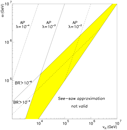
Figure 1: Region of parameters in the $(v_{R},\omega)$ plane that could lead to a majoron decay of the $\tau$ lepton with BR of the order $10^{-6}-10^{-4}$ in the see-saw approximation.

The above semi-analytic estimates are illustrated in figure 1. We display the region of relevant scale parameters $(v_{R},\omega)$ that could lead to $\tau$ decays to majorons with BR of the order $10^{-6}-10^{-4}$. We assume that the product of the relevant Yukawa couplings and diagonalizing matrix elements is of order $10^{-1}$. The restrictions, shown as lines in the plot, come from the astrophysical constraint of eq. (9), the requirement upon the BR and the see-saw limit approximation (one should have at least $\omega^{2}\raise 1.29167pt\hbox{$\;>$\kern-7.5pt\raise-4.73611pt\hbox{$\sim\;$}}v_{R}^{2}$). The condition from astrophysics requires $v_{R}$ and $\omega$ to be on the right side of the lines labelled with AP, shown for three different values of the parameter $\lambda$ in eq. (8). On the other hand the BR of the majoron process can be larger than $10^{-6}$ ($10^{-4}$) for values of the scales below the thick solid (dashed) line. For definiteness, the shaded region corresponds to BR larger than $10^{-6}$ for $\lambda\geq 10^{-3}$.

4.1 Numerical Results

Parameter	Range
$\lambda$	$10^{-4}\rightarrow 1$
$\omega$	$10^{4}\rightarrow 10^{8}$ GeV
$v_{R}$	$10^{3}\rightarrow 10^{8}$ GeV
Yukawas	$10^{-5}\rightarrow 10^{-2}$

Table 2: Ranges of variation of the different parameters used in our numerical calculations.

We now turn to a more accurate determination of the expected branching ratios for the majoron emitting $\tau$ and $\mu$ decays, for the more general case in which the hierarchy of scales used in the seesaw approximation is relaxed. In order to do this we have performed the numerical calculation of the off-diagonal elements of the majoron couplings matrix in eq. (22) in the case that the ratio $v_{R}/\omega$ is left arbitrary (no see-saw). The various parameters such as $\lambda$, the symmetry breaking scales and Yukawa couplings were randomly varied in certain reasonable ranges given in Table 2, and the scales $v$ and $v_{L}$ are fixed by eq. (8) and the light $W$ boson mass. For those choices which were not in conflict with the astrophysical bound of eq. (9), we have calculated the corresponding branching ratios for the lepton-flavour-violating decays of eq. (1). Our results for tau are summarized in Fig. 2 for the two possible channels and in Fig. 3 for the $\mu\to e+J$ case for four different ranges of $\lambda$ values. The points represent pairs of ($v_{R},\omega$) values which lead to the branching ratios larger than indicated.

Figure 2: Allowed regions in the $v_{R}-\omega$ plane for $\tau$ decays.

Figure 3: Allowed regions in the $v_{R}-\omega$ plane for $\mu$ decays.

Clearly the $\tau\to eJ$ branching ratios can reach or even exceed $10^{-5}$. These values are in principle within reach of a possible tau-charm factory which could obtain the limits $B(\tau\rightarrow eJ)<10^{-5}$ (standard optics) or $B(\tau\rightarrow eJ)<10^{-6}$ (monochromator [25]). For the $\tau\to\mu J$ case the branching ratios allowed in our model can reach or even exceed $10^{-4}$. Though the attainable sensitivity in this case is $B(\tau\rightarrow\mu J)<10^{-3}$, which is limited by $\mu/\pi$ separation, it may in principle be improved by an order of magnitude with a RICH detector. For a discussion see ref. [21] and references therein.

The allowed $\mu\to eJ$ branching ratios are illustrated in Fig. 3 for various choices of the range of variation of $\lambda$. The present experimental limit from TRIUMF [17] on $\mu\to e+J$ is $BR(\mu\to e+J)\leq 2.6\times 10^{-6}$. One sees that for the most favorable case studied, $\lambda\geq 10^{-4}$ we find that the $\mu\to eJ$ branching ratios can reach or exceed $10^{-6}$ which is quite close to the present limit. Presumably this could be improved either at TRIUMF or PSI.

5 Discussion and Conclusions

We have proposed in this paper an extension of the $SU(2)_{L}\otimes SU(2)_{R}\otimes U(1)_{B-L}$ Left-Right symmetric gauge model for the electroweak interaction in which a global $U(1)_{G}$ lepton-number-like symmetry is postulated. Its spontaneous breaking at a scale $\omega\raise 1.29167pt\hbox{$\;>$\kern-7.5pt\raise-4.73611pt\hbox{$\sim\;$}}10^{4}$ GeV or so would give rise to interesting physical effects associated to the corresponding physical Nambu-Goldstone boson, called majoron (denoted $J$). Due to the existence of lepton-number-carrying heavy isosinglet leptons $E_{i}$ there can be tree-level flavour-violating majoron-charged-lepton couplings, leading to sizeable majoron-emitting lepton-flavour-violating muon and tau decays. We have discussed explicitly a simplest version of the model and showed that the branching ratios for $\mu\to e+J$, $\tau\to e+J$ and $\tau\to\mu+J$ decays can be large enough to fall within the sensitivities of future $\mu$ and $\tau$ factories. On the other hand the left-right gauge symmetry breaking scale may be as low as few TeV. A simple variant of the model can be considered in which isosinglet quarks instead of leptons are introduced, in which case one would expect similar effects in the decays of hadrons, such as K mesons.

Before concluding, note that the presence of the isosinglet charged leptons $E_{i}$ also leads to flavour-violating couplings of the light charged leptons to the neutral gauge bosons $Z_{1,2}$ present in the model, already at the tree level. These would lead also to more standard lepton-flavour-violating decays such as $\tau\to 3e$, $\tau\to 3\mu$, etc. Such decays are potentially interesting both for a tau-charm factory as well as for a B meson factory [21]. However, we have investigated the corresponding lepton-flavour-violating couplings to neutral gauge bosons in our model and have found that the they are suppressed by factors of $v_{L}/\omega\approx 10^{-5}$. This would lead to effects which are too small to observe. Finally, photon emitting lepton-flavour-violating decays such as $\mu\to e+\gamma$ in left-right symmetric models have been widely discussed in the literature. We avoid their discussion as it would require the specification of the neutral lepton sector so that the corresponding predictions would be more model-dependent. We conclude that the search for lepton-flavour-violating majoron-emitting weak decays provides a most sensitive way of testing our model.

Appendix A Appendix

In this appendix we consider an alternative, more elegant and more general method to derive the off-diagonal couplings of the charged leptons to the majoron. This method is a two-fold generalization of the one given in ref. [19]. Firstly, it is generalized to the case of Dirac fermions, and secondly, and more importantly, it is generalized to the case where the majoron gets contributions from the neutral components of more than one scalar multiplet.

The first step is to write down the Noether current of the charged leptons in the weak basis and the scalars corresponding to each conserved charge. Here we need consider only the currents which are themselves electrically neutral. This gives us the equations

$$J_{\mu}^{A}=\sum^{N}_{i=1}\left(\bar{l}_{iL}\gamma_{\mu}l_{iL}g_{iL}^{A}+\bar{l}_{iR}\gamma_{\mu}l_{iR}g_{iR}^{A}+\bar{E}_{iL}\gamma_{\mu}E_{iL}G_{iL}^{A}+\bar{E}_{iR}\gamma_{\mu}E_{iR}G_{iR}^{A}\right)$$

$$+\sum_{a}\phi_{a}^{R}\stackrel{{\scriptstyle\leftrightarrow}}{{\partial}}_{\mu}\phi_{a}^{I}g_{a}^{A}$$ (28)

Here $A$ stands for each independent charge, the index $i$ runs over lepton flavours, and $a$ runs over the various neutral scalar fields. The superscripts R and I refer to the real and imaginary parts of the scalar fields, respectively. $g_{i}^{A}$ and $G_{i}^{A}$ are the charges of the fields $l_{i}$ and $E_{i}$, with L and R denoting the chiralities, and $g_{a}^{A}$ are the charges of the scalar fields.

Conservation of the Noether currents corresponds to the equation

$$\partial^{\mu}\left[\sum^{N}_{i=1}\left(\bar{l}_{iL}\gamma_{\mu}l_{iL}g_{iL}^{A}+\bar{l}_{iR}\gamma_{\mu}l_{iR}g_{iR}^{A}+\bar{E}_{iL}\gamma_{\mu}E_{iL}G_{iL}^{A}+\bar{E}_{iR}\gamma_{\mu}E_{iR}G_{iR}^{A}\right)\right]$$

$$+\sum_{a}\langle\phi_{a}^{R}\rangle\Box\phi_{a}^{I}g_{a}^{A}=0$$ (29)

at the semiclassical level. In the case when the scalar field carry only a single non-zero charge $g^{A}$, the combination $\langle\phi_{a}^{R}\rangle\phi_{a}^{I}g_{a}^{A}$ is the majoron field $J$, apart from a normalization factor. The above equation then directly gives the coupling of the majoron to the various leptonic fields, using Lagrange’s equation

$$\Box J=-\frac{\partial{\cal L}_{J}}{\partial J},$$ (30)

and the Dirac equation on the left-hand side for the various fermionic fields. In the general case, the majoron is a linear combination

$$J=\sum_{a}\langle\phi_{a}^{R}\rangle\phi_{a}^{I}(\sum_{A}\alpha_{A}g_{a}^{A}),$$ (31)

In that case, multiplying eq. (A) by $\alpha_{A}$ and summing over $A$ we get

$$\partial^{\mu}\left[\sum_{i,A}\alpha_{A}\left(\bar{l}_{iL}\gamma_{\mu}l_{iL}g_{iL}^{A}+\bar{l}_{iR}\gamma_{\mu}l_{iR}g_{iR}^{A}+\bar{E}_{iL}\gamma_{\mu}E_{iL}G_{iL}^{A}+\bar{E}_{iR}\gamma_{\mu}E_{iR}G_{iR}^{A}\right)\right]+\Box J=0.$$ (32)

Again using eq. (30) the above equation gives the majoron couplings in terms of the weak basis fields. To get the result for the off-diagonal couplings, we first use the Dirac equation for the fermionic fields to get

$$-i\sum_{A}\alpha_{A}(\!\begin{array}[]{cc}\bar{l}_{L}&\bar{E}_{L}\end{array}\!)\left\{\left(\begin{array}[]{cc}g_{L}^{A}\,I&0\\ 0&G_{L}^{A}\,I\end{array}\right)M-M\left(\begin{array}[]{cc}g_{R}^{A}\,I&0\\ 0&G_{R}^{A}\,I\end{array}\right)\right\}\left(\begin{array}[]{c}l_{R}\\ E_{R}\end{array}\right)+h.c.-\frac{\partial{\cal L}}{\partial J}=0.$$ (33)

On expressing the weak basis fields in terms of the diagonal fields, this would give the complete expression for the leptonic majoron couplings. However, if we are interested only in the off-diagonal couplings, we can achieve a simplification by noting that if the quantum numbers $g$ and $G$ in the above equation were equal, the couplings of the majoron would be just proportional to the mass matrices, and therefore diagonal. Hence the deviation from diagonality of the couplings would be proportional to the differences between $g$ and $G$. Using this fact, the equation for the off-diagonal couplings then reduces to:

$${\cal L}^{J}_{off-diag}=-iJ\sum_{A}\alpha_{A}\\ (\!\begin{array}[]{cc}\bar{l}_{L}&\bar{E}_{L}\end{array}\!)\left\{\left(\begin{array}[]{cc}0&0\\ 0&\delta g_{L}^{A}\,I\end{array}\right)M-M\left(\begin{array}[]{cc}0&0\\ 0&\delta g_{R}^{A}\,I\end{array}\right)\right\}\left(\begin{array}[]{c}l_{R}\\ E_{R}\end{array}\right)+h.c.,$$ (34)

where

$$\delta g_{L}^{A}=G_{L}^{A}-g_{L}^{A};\quad\delta g_{R}^{A}=G_{R}^{A}-g_{R}^{A}.$$ (35)

Using the relations between the weak and mass basis states for the light leptons we then get the off-diagonal majoron couplings as

$${\cal L}^{J}_{off-diag}=-iJ\sum_{A}\alpha_{A}\bar{e}_{iL}(T_{L})_{ij}\{\left[(V_{L})_{12}(V_{L})^{\dagger}_{12}\right]_{jk}m_{k}(G_{L}^{A}-g_{L}^{A})-$$

$$-m_{i}(G_{R}^{A}-g_{R}^{A})\left[(V_{R})_{21}(V_{R})^{\dagger}_{21}\right]_{jk}\}(T_{R})^{\dagger}_{kl}e_{lR}+h.c.$$ (36)

Knowing the diagonalizing matrices $T_{L}$, $T_{R}$, $V_{L}$ and $V_{R}$ in a specific model, the off-diagonal couplings can easily be calculated.

We illustrate this method for the case at hand. In our specific model, the various independent conserved charges can be chosen as the global $U(1)$ charge, $B-L$ and the combination $T_{3L}-T_{3R}$. The quantum numbers of the various fields are given in Table 1. The majoron is the linear combination of the neutral scalar fields given in eq. (4). This implies the values of $\alpha_{A}$ as follows:

$$\alpha_{1}=\frac{1}{N},\;\;\alpha_{2}=\frac{v^{2}(v_{L}^{2}-v_{R}^{2})}{V^{2}v_{R}^{2}rN},\;\;\alpha_{3}=\frac{-2v_{L}^{2}}{V^{2}rN},$$ (37)

where

$$N=2(\omega^{2}+\frac{v_{L}^{2}v_{R}^{2}v^{2}}{V^{2}v_{R}^{2}+v^{2}v_{L}^{2}})^{-\frac{1}{2}}.$$ (38)

Substituting these values and the various quantum numbers in eq. (36) gives

$${\cal L}^{J}_{off-diag}=-iJ\bar{e}_{iR}\{m_{k}\left(T_{L}(V_{L})_{12}(V_{L})_{12}^{\dagger}T_{R}^{\dagger}\right)_{ik}\left(\frac{-2v_{L}^{2}(v^{2}+v_{R}^{2})}{v_{R}^{2}V^{2}r}\right)$$

$$-m_{i}\left(T_{L}(V_{R})_{12}(V_{R})_{12}^{\dagger}T_{R}^{\dagger}\right)_{ik}\left(\frac{2}{r}\right)\}e_{kL}+h.c.$$ (39)

The final result given in eq. (24) can then be obtained on substituting for $V_{L}$ and $V_{R}$ from eq. (14) and eq. (15).

References

- [1] J.C. Pati and A. Salam, Phys. Rev. D 10 (1975) 275; R.N. Mohapatra and J.C. Pati, Phys. Rev. D 11 (1975) 566, Phys. Rev. D 11 (1975) 2558.
- [2] R.N. Mohapatra and G. Senjanović, Phys. Rev. D 23 (1981) 165.
- [3] S. Gerstein and Ya.B. Zeldovich, Zh. Eksp. Teor. Fiz. Pisma. Red. 4 (1966) 174; R. Cowsik and J. McClelland, Phys. Rev. Lett. 29 (1972) 669; D. Dicus et al., Astrophys. J. 221 (1978) 327; B.W. Lee and S. Weinberg, Phys. Rev. Lett. 39 (1977) 165.
- [4] Y. Chikashige, R.N. Mohapatra and R. Peccei, Phys. Rev. Lett. 45 (1980) 1926; Phys. Lett. B 98 (1981) 265.
- [5] J.W.F. Valle, Phys. Lett. B 131 (1983) 87; G. Gelmini and J.W.F. Valle, Phys. Lett. B 142 (1984) 181; J.W.F. Valle, Phys. Lett. B 159 (1985) 49; M.C. González-García and J.W.F. Valle, Phys. Lett. B b216 (1989) 360; A. Joshipura and S. Rindani, Phys. Rev. D 46 (1992) 3000.
- [6] M.C. González-García and J.W.F. Valle, Phys. Lett. B 216 (1989) 360.
- [7] J.W.F. Valle, Gauge Theories and the Physics of Neutrino Mass, Prog. Part. Nucl. Phys. 26 (1991) 91-171 and references therein.
- [8] A.D. Dolgov, S. Pastor, J.C. Romão and J.W.F. Valle, Nucl. Phys. B 496 (1997) 24.
- [9] M. Kawasaki et al., Nucl. Phys. B 419 (1994) 105; S. Dodelson, G. Gyuk and M.S. Turner, Phys. Rev. D 49 (1994) 5068; S. Hannestad, Phys. Rev. D 57 (1998) 2213; M. Kawasaki et al. , K. Kohri and K. Sato, Phys. Lett. B 430 (1998) 132.
- [10] G. Raffelt, Stars as Laboratories for Fundamental Physics (The University of Chicago Press, 1996).
- [11] E.Kh. Akhmedov, A.S. Joshipura, S. Ranfone and J.W.F. Valle, Nucl. Phys. B 441 (1995) 61; for an early alternative proposal in this direction see, A. Kumar and R.N. Mohapatra, Phys. Lett. B 150 (1985) 191.
- [12] S. Kalara and K.A. Olive, Nucl. Phys. B 331 (1990) 181; J. Distler, B.R. Greene, K.H. Kirklin, and P.J. Miron, Commun. Math. Phys. 122 (1989) 117.
- [13] V. Barger, N.G. Deshpande, and K. Hagiwara, Phys. Rev. D 36 (1987) 3541; Int. J. Mod. Phys. A 2 (1987) 1181.
- [14] V. Barger et al in Proceedings, Physics of the Superconducting Supercollider, Snowmass 1986, p. 216-220.
- [15] A. Davidson and K. C. Wali, Phys. Rev. Lett. 59 (1987) 393. For a recent paper see, e.g. Yoshio Koide, Phys. Rev. D 57 (1998) 5836 and references therein.
- [16] J. C. Romão, N. Rius and J. W. F. Valle, Nucl. Phys. B 363 (1991) 369.
- [17] A. Jodidio et al., Phys. Rev. D 34 (1986) 1967.
- [18] MARK III Collaboration, Phys. Rev. Lett. 55 (1985) 1842.
- [19] J. Schechter and J.W.F. Valle, Phys. Rev. D 25 (1982) 774.
- [20] For a recent experimental discussion of tau decays by the CLEO collaboration, see Phys. Rev. D 57 (1998) 5903.
- [21] For a discussion of the experimental prospects for detecting lepton-flavour-violating muon and tau decays at future B and tau-charm factories see Searching for Exotic Tau Decays, by R. Alemany, J.J. Gómez-Cadenas, M.C. González-García and J.W.F. Valle, preprint hep-ph/9307252 or CERN-PPE/93-49 and references therein.
- [22] R.N. Mohapatra and J.W.F. Valle, Phys. Rev. D 34 (1986) 1642; I. Antoniadis et al., Phys. Lett. B 208 (1988) 209; E. Papageorgiu and S. Ranfone, Phys. Lett. B 282 (1992) 89.
- [23] D. Wyler and L. Wolfenstein, Nucl. Phys. B 218 (1983) 205.
- [24] For a review see J.E. Kim, Phys. Rept. 150 (1987) 1.
- [25] See for example, A. Faus-Golfe and J. Le Duff, Report LAL/RT 92-01 (1992).