Light-cone Variables, Rapidity and All That

Abstract

I give a pedagogical summary of the methods of light-cone variables, rapidity and pseudo-rapidity. Then I show how these methods are useful in analyzing diffractive high-energy collisions.

I Introduction

The use of light-cone variables, rapidity and pseudo-rapidity is very common in treating high-energy scattering, particularly in hadron-hadron and lepton-hadron collisions. The essential features of these collisions that make these variables of utility are the presence of ultra-relativistic particles and a preferred axis.

In these notes I will explain the theory of these variables. The only prerequisites are a knowledge of the elements of special relativity and an acquaintance with the general phenomenological features of high-energy scattering. Then I will show how these variables can be used conveniently in the analysis of the kinematics of diffractive processes. This will include the derivation of an approximate relation between the size of the rapidity gap and the variable $x_{\mathbb{P}}$.

The material in these notes is essentially all standard and well known to many workers in the field. But it is not always easy to find the material conveniently presented.

II Light-cone coordinates, rapidity

A Definitions

Light-cone coordinates are defined by a change of variables from the usual $(t,x,y,z)$ (or $(0,1,2,3)$) coordinates. Given a vector $V^{\mu}$, its light-cone components are defined by

$$V^{+}=\frac{V^{0}+V^{3}}{\sqrt{2}},{}~{}~{}~{}V^{-}=\frac{V^{0}-V^{3}}{\sqrt{2}},{}~{}~{}~{}{\bf V}^{T}=(V^{1},V^{2}),$$ (1)

and I will write $V^{\mu}=(V^{+},V^{-},{\bf V}^{T})$. Some authors prefer to omit the $1/\sqrt{2}$ factor in Eq. (1). It can easily be verified that Lorentz invariant scalar products have the form

$$V\cdot W = V^{+}W^{-}+V^{-}W^{+}-{\bf V}_{T}\cdot{\bf W}_{T},$$ (2)

$$V\cdot V = 2V^{+}V^{-}-V_{T}^{2}.$$ (3)

What are the motivations for defining such coordinates, which evidently depend on a particular choice of the $z$ axis? One is that these coordinates transform very simply under boosts along the $z$-axis. Another is that when a vector is highly boosted along the $z$ axis, light-cone coordinates nicely show what are the large and small components of momentum. Typically one uses light-cone coordinates in a situation like high-energy hadron scattering. In that situation, there is a natural choice of an axis, the collision axis, and one frequently needs to transform between different frames related by boosts along the axis. Commonly used frames include the rest frame of one of the incoming particles, the overall center-of-mass frame, and the center-of-mass of a partonic subprocess.

B Boosts

Let us boost the coordinates in the $z$ direction to make a new vector $V^{\prime\mu}$. In the ordinary $(t,x,y,z)$ components we have the well known formulae

$$V^{\prime 0}=\frac{V^{0}+vV^{z}}{\sqrt{1-v^{2}}},{}~{}~{}~{}V^{\prime z}=\frac{vV^{0}+V^{z}}{\sqrt{1-v^{2}}},{}~{}~{}~{}V^{\prime x}=V^{x},{}~{}~{}~{}V^{\prime y}=V^{y}.$$ (4)

It is easy to derive the following for the light-cone components:

$$V^{\prime+}=V^{+}{\rm e}^{\psi},{}~{}~{}~{}V^{\prime-}=V^{-}{\rm e}^{-\psi},{}~{}~{}~{}{\bf V^{\prime}}_{T}={\bf V}_{T},$$ (5)

where the hyperbolic angle $\psi$ is $\frac{1}{2}\ln\frac{1+v}{1-v}$, so that $v=\tanh\psi$.

Notice that if we apply two boosts of parameters $\psi_{1}$ and $\psi_{2}$ the result is a boost $\psi_{1}+\psi_{2}$. This is clearly simpler than the corresponding result expressed in terms of velocities.

C Rapidity

a Boost of particle momentum

Consider a particle of mass $m$ that is obtained by a boost $\psi$ from the rest frame. Its momentum is

$$p^{\mu} = \left(p^{+},\frac{m^{2}}{2p^{+}},{\bf 0}_{T}\right)$$ (6)

$$= \left(\frac{m}{\sqrt{2}}{\rm e}^{\psi},\frac{m}{\sqrt{2}}{\rm e}^{-\psi},{\bf 0}_{T}\right)$$ (7)

Notice that if the boost is very large (positive or negative), only one of the two non-zero light-cone components of $p^{\mu}$ is large; the other component becomes small. With the usual components two of the components, $p^{0}$ and $p^{z}$, become large.

Suppose next that we have two such particles, $p_{1}$ and $p_{2}$, with the boost for particle 1 being much larger than that for particle 2. Then in the scalar product of the two momenta only one component of each momentum dominates the result, thus for example $(p_{1}+p_{2})^{2}\simeq 2p_{1}^{+}p_{2}^{-}$. This implies that, when analyzing the sizes of scalar products of highly boosted particles, it is simpler to use light-cone components than to use conventional components.

b Definition of rapidity

Since the ratio $p^{+}/p^{-}$ gives a measure ${\rm e}^{2\psi}$ of the boost from the rest frame, we are led to the following definition of a quantity called “rapidity”:

$$y=\frac{1}{2}\ln\frac{p^{+}}{p^{-}}=\frac{1}{2}\ln\frac{E+p^{z}}{E-p^{z}},$$ (8)

which can be applied to a particle of non-zero transverse momentum. The 4-momentum of a particle of rapidity $y$ and transverse momentum ${\bf p}_{T}$ is

$$p^{\mu}=\left(\sqrt{\frac{m^{2}+p_{T}^{2}}{2}}\,{\rm e}^{y},\sqrt{\frac{m^{2}+p_{T}^{2}}{2}}\,{\rm e}^{-y},{\bf p}_{T}\right),$$ (9)

with $\sqrt{m^{2}+p_{T}^{2}}$ being called the transverse energy $E_{T}$ of the particle. It can be checked that the scalar product of two momenta is

$$p_{1}\cdot p_{2}=E_{1T}E_{2T}\cosh(y_{1}-y_{2})-{\bf p}_{1T}\cdot{\bf p}_{2T}.$$ (10)

In the case where the transverse momenta are negligible, this reduces to $m^{2}\cosh(y_{1}-y_{2})$, which is like the formula for the product of two Euclidean vectors ${\bf p}_{1}\cdot{\bf p}_{2}=p_{1}p_{2}\cos\theta$, with the trigonometric cosine being replaced by the hyperbolic cosine.

c Transformation under boosts

Under a boost in the $z$ direction, rapidity transforms additively:

$$y\to y^{\prime}=y+\psi.$$ (11)

This implies that in situations where we have a frequent need to work with boosts along the $z$ axis it is economical to label the momentum of a particle by its rapidity and transverse momentum, rather than to use 3-momentum.

d Rapidity distributions in high-energy collisions

It also happens that in most collisions in high-energy hadronic scattering, the distribution of final-state hadrons is approximately uniform in rapidity, within kinematic limits. That is, the distribution of final-state hadrons is approximately invariant under boosts in the $z$ direction. This implies that rapidity and transverse momentum are appropriate variables for analyzing data and that detector elements should be approximately uniformly spaced in rapidity. (What is physically possible is to make a detector uniform in the angular variable pseudo-rapidity that I will discuss below.) This is in contrast to the situation for $e^{+}e^{-}$ collisions where most of the interest is in events generated via annihilation into an electro-weak boson. Such events are much closer to uniform in solid angle than uniform in rapidity.

e Non-relativistic limit

Observe that for a non-relativistic particle, rapidity is the same as velocity along the $z$-axis, for then

$$y = \frac{1}{2}\ln\frac{E+p^{z}}{E-p^{z}}\simeq\frac{1}{2}\ln\frac{m+mv^{z}}{m-mv^{z}}=v^{z}.$$ (12)

Non-relativistic velocities transform additively under boosts, and the non-linear change of variable from velocity to rapidity allows this additive rule Eq. (11) to apply to relativistic particles (but only in one direction of boost).

One way of seeing this is as follows: The relativistic law for addition of velocities in one dimension is

$$\beta_{13}=\frac{\beta_{12}+\beta_{23}}{1+\beta_{12}\beta_{23}},$$ (13)

where $\beta_{12}$ is the velocity of some object 1 measured in the rest-frame of object 2, etc. This formula is reminiscent of the following property of hyperbolic tangents:

$$\tanh(A+B)=\frac{\tanh A+\tanh B}{1+\tanh A\tanh B}.$$ (14)

So to obtain a linear addition law, we should write $\beta_{12}=\tanh A_{12}$, and then the rule Eq. (13) for the addition of velocities becomes simply $A_{13}=A_{12}+A_{23}$. The $A$ variables are exactly relative rapidities, since

$$v^{z}=\frac{p^{z}}{E}=\frac{p^{+}-p^{-}}{p^{+}+p^{-}}=\tanh y.$$ (15)

f Relative velocity

Rapidity is the natural relativistic velocity variable. Suppose we have a proton and a pion with the same rapidity at $p_{T}=0$. Then they have no relative velocity; to see this, one just boosts to the rest frame of one of the particles. But these same particles have very different energies: $E_{p}=\frac{m_{p}}{m_{\pi}}E_{\pi}$.

D Pseudo-rapidity

As I will now explain, the rapidity of a particle can easily be measured in a situation where its mass is negligible, for then it is simply related to the polar angle of the particle.

First let us define the pseudo-rapidity of a particle by

$$\eta=-\ln\tan\frac{\theta}{2},$$ (16)

where $\theta$ is the angle of the 3-momentum of the particle relative to the $+z$ axis. It is easy to derive an expression for rapidity in terms of pseudo-rapidity and transverse momentum:

$$y=\ln\frac{\sqrt{m^{2}+p_{T}^{2}\cosh^{2}\eta}+p_{T}\sinh\eta}{\sqrt{m^{2}+p_{T}^{2}}}.$$ (17)

In the limit that $m\ll p_{T}$, $y\to\eta$. This accounts both for the name ‘pseudo-rapidity’ and for the ubiquitous use of pseudo-rapidity in high-transverse-momentum physics. Angles, and hence pseudo-rapidity, are easy to measure. But it is really the rapidity that is of physical significance: for example the distribution of particles in a minimum bias event is approximately uniform in rapidity over the kinematic range available.

The distinction between rapidity and pseudo-rapidity is very clear when one examines the kinematic limits on the two variables. In a collision of a given energy, there is a limit to the energy of the particles that can be produced. This can easily be translated to limits on the rapidities of the produced particles of a given mass. But there is no limit on the pseudo-rapidity, since a particle can be physically produced at zero angle (or at $180^{\circ}$), where its pseudo-rapidity is infinite. The particles for which the distinction is very significant are those for which the transverse momentum is substantially less than the mass. Note: from Eq. (17) it follows that $y<\eta$ always.

III Diffractive Scattering

A Kinematics

Let us define a single diffractive collision as one in which one of the beam particles emerges almost unscathed from the scattering, with only a small deflection and a small loss of energy (Fig. 1):

$$p+\bar{p}\to p^{\prime}+X.$$ (18)

For the sake of definiteness, I have assumed a proton-antiproton collision with the proton being diffracted. One can treat any other collision in the same fashion. Indeed, replacing the incoming and outgoing protons by electrons gives us electroproduction processes, and the low $Q^{2}$ events that are used to measure photoproduction cross sections have exactly the same kinematic properties as diffractive hadron collisions.

Suppose the particle $p$ is moving in the $+z$ direction, and $\bar{p}$ in the opposite direction. Then we define the kinematics in terms of the transverse momentum ${\bf p^{\prime}}_{T}$ of the diffracted hadron and a variable $x_{\mathbb{P}}$ defined as $1-p^{\prime+}/p^{+}$. Thus the components of $p$ and $p^{\prime}$ are

$$p^{\mu} = \left(p^{+},\frac{m^{2}}{2p^{+}},{\bf 0}_{T}\right),$$ (19)

$$p^{\mu} = \left((1-x_{\mathbb{P}})p^{+},\frac{m^{2}+{p^{\prime}}_{T}^{2}}{2(1-x_{\mathbb{P}})p^{+}},{\bf p^{\prime}}_{T}\right).$$ (20)

It is convenient to examine the momentum transfer:

$$\Delta^{\mu}\equiv p^{\mu}-p^{\prime\mu}=\left(x_{\mathbb{P}}p^{+},-\frac{x_{\mathbb{P}}m^{2}+{p^{\prime}}_{T}^{2}}{2(1-x_{\mathbb{P}})p^{+}},-{\bf p^{\prime}}_{T}\right).$$ (21)

Clearly, $x_{\mathbb{P}}$ represents a fractional loss of the $+$ component of momentum. When the two protons are both moving fast, this fraction is also the fractional energy loss: $x_{\mathbb{P}}=1-E^{\prime}/E+O(1/E)$; but the definition in light cone components converts this to a boost-invariant definition. The invariant momentum transfer is

$$t=\Delta^{2} = -\frac{{p^{\prime}}_{T}^{2}+x_{\mathbb{P}}^{2}m^{2}}{1-x_{\mathbb{P}}}$$ (22)

$$\to -{p^{\prime}}_{T}^{2}\mbox{~{}as $x_{\mathbb{P}}\to 0$}.$$ (23)

Thus at small $x_{\mathbb{P}}$, $t$ is an equivalent variable to the transverse momentum of the outgoing diffracted hadron.

FIG. 1.: Diffractive scattering.

The diffractive region is when $x_{\mathbb{P}}$ is small enough that the power law attributed to pomeron exchange dominates. The exact nature of the pomeron in QCD is still quite uncertain. But from a practical point-of-view one can identify it with whatever is exchanged between hadrons to make the approximately constant total cross sections that are observed at high-energy. The object exchanged between the protons in Fig. 1 and the system labeled $X$ is a pomeron when $x_{\mathbb{P}}$ is sufficiently small. In the Regge phenomenology of diffractive scattering, this is associated with an $x_{\mathbb{P}}$ distribution of the events that is approximately $dx_{\mathbb{P}}/x_{\mathbb{P}}$.

A more general definition of diffraction is that it consists of events in which there are non-exponentially suppressed rapidity gaps. The events that are diffractive in the first definition in fact are also diffractive according to the second definition. As I will show in Sect. III E, events with small $x_{\mathbb{P}}$ have a rapidity gap that grows like $\ln(1/x_{\mathbb{P}})$. The power law associated with pomeron exchange gives a distribution of events that is approximately $dx_{\mathbb{P}}/x_{\mathbb{P}}$, and hence approximately a constant distribution in the size of the rapidity gap. That is, it gives non-exponentially suppressed rapidity gaps.

In contrast, if one has a statistical distribution of particles, uniform in rapidity, and if all the correlations between particles are local in rapidity, then the probability of a rapidity gap of size $\Delta y$ is proportional to $e^{-a\Delta y}$, for some constant $a$. Experimental data, for example, Fig. 2 indicate that for small gaps there is indeed an approximately exponential fall-off with increasing $\Delta y$. But for large enough gaps, more than 2 or 3 units, a presumably different mechanism of particle production becomes significant, and there is no longer a strong exponential drop. Of course, once $\Delta y$ gets close to the kinematic limit, the distribution in $\Delta y$ must decrease again.

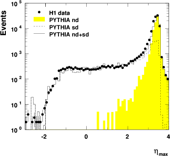
FIG. 2.: Distribution of $\eta_{\rm max}$ in photoproduction at H1 [1]. There are no detected particles with pseudo-rapidity between $\eta_{\rm max}$ at the end of the detector at $\eta=3.65$

Strictly speaking, one should not talk about specific events as being diffractive or non-diffractive. Instead one should talk about the diffractive and non-diffractive components of a cross-section. When one says that a specific event is diffractive, one really means that it is in a kinematic region (of $x_{\mathbb{P}}$ or rapidity gap) where diffraction is the dominant contribution to the cross section.

B Existence of a rapidity gap

Now the maximum value of the $+$ component of the momentum of a hadron in the $X$ part of the final state in (18) is $\Delta^{+}=x_{\mathbb{P}}p^{+}$. It then follows from Eq. (9) that the maximum possible value of rapidity for any particle in $X$ is

$$y_{\rm kin.\ max}=\ln\frac{2x_{\mathbb{P}}E}{m},$$ (24)

where $E$ is the beam energy (assumed to be much larger than the proton mass).

For a numerical example, consider a diffractive process with an incoming proton of energy 900 GeV (as at the Fermilab Tevatron), and with $x_{\mathbb{P}}=0.01$, a value typically considered to be safely in the diffractive region. The incoming proton itself has rapidity 7.6. From Eq. (24) the maximum possible rapidity of pions in the event is 4.9. There is therefore a rapidity gap on the proton side of the event. Since there are normally many particles in the event, which share the momentum, the edge of the rapidity gap, $y_{\rm max}$, will typically be a unit or more lower.

The distribution of the soft particles in a hadronic collision is approximately uniform in rapidity. So when the final-state particles are plotted in azimuth $\phi$ and rapidity $y$, a diffractive event therefore looks like Fig. 3. When $x_{\mathbb{P}}$ is decreased, the value of $y_{\rm kin.\ max}$ also decreases, and hence the size of the rapidity gap increases.

FIG. 3.: Plot of the distribution of final-state particles in a typical diffractive event is uniform in $\phi$ and $y$ except for an isolated forward proton.

C Computation of $x_{\mathbb{P}}$ from the non-diffracted part of the final state

In principle, $x_{\mathbb{P}}$ can be either measured from the final state hadron: $x_{\mathbb{P}}=1-p^{\prime+}/p^{+}$ or from the rest of the final state:

$$x_{\mathbb{P}}=\sum_{i\epsilon X}\frac{k_{i}^{+}}{p^{+}},$$ (25)

where the sum is over all particles in the remaining part $X$ of the final state.

To measure $x_{\mathbb{P}}$ from the diffracted hadron requires first that there be elements of the detector (e.g., Roman pots) close to the beam-pipe, which is not always the case. Moreover, if $x_{\mathbb{P}}$ is very small, the hadron’s energy needs to be known very precisely to obtain a useful accuracy on $x_{\mathbb{P}}$; if the measurement is not sufficiently accurate, one cannot distinguish the value from zero. (Values of $x_{\mathbb{P}}$ in the range $10^{-4}$ to $10^{-2}$ are often discussed.) So if a useful measurement of $x_{\mathbb{P}}$ is not available, one must measure the rest of the hadronic final-state, and deduce $x_{\mathbb{P}}$ by using Eq. (25).

In principle, the use of Eq. (25) requires knowledge of all the (typically many) particles in $X$. One might imagine that poor information on $X$, for example from a lack of calorimetry in the backward part of the detector, would prevent such a measurement from being practical.

In fact, as I will now show, the value of the right-hand-side of Eq. (25) is dominated by the particles of the largest $k_{T}$ (i.e., jet particles), and by the particles that are closest in rapidity to the diffracted hadron, i.e., closest to the edge of the rapidity gap.

We simply write each $k_{i}^{+}$ in Eq. (25) in terms of rapidity and transverse momentum to obtain

$$x_{\mathbb{P}}=\sum_{i\epsilon X}\frac{E_{iT}{\rm e}^{y_{i}}}{2E}.$$ (26)

Here I have approximated $p^{+}$ by $E\sqrt{2}$, with $E$ being the energy of the incoming proton, which is assumed to be large. The transverse momentum appears in form of the transverse energy $E_{iT}=\sqrt{k_{iT}^{2}+m^{2}}$. We next recall that particles in a hadronic scattering event are typically uniformly distributed in rapidity between some kinematic limits, and have a steeply falling spectrum in transverse momentum. The exponential of rapidity in Eq. (26) therefore implies that the sum is dominated by those particles of the highest rapidity.

The exception to this statement is given by particles that result from a hard scattering and that therefore have large transverse momentum. Hence the general statement is that the sum in Eq. (26) is dominated by (a) particles with the largest rapidity (i.e., closest to the edge of the rapidity gap), and (b) particles with high transverse momentum. This means that the measurement can be effectively be made from

$$x_{\mathbb{P}}\simeq\sum_{{\rm particles\ with\ highest\ }y\atop{\rm particles\ with\ large\ }E_{T}}\frac{E_{iT}{\rm e}^{y_{i}}}{2E}.$$ (27)

Hence a lack of detector coverage on the opposite side to the diffracted proton does not greatly affect the accuracy of the measurement.

Exactly this method is used in a corresponding problem in deep-inelastic scattering, where it is known as the Jacquet-Blondel [2] method. There it is desired to measure the scaling variable $y$ (which has no relation to rapidity). This variable is defined in terms of the scattered lepton in exactly the way in which our $x_{\mathbb{P}}$ is defined in terms of the diffracted proton. By momentum conservation, $y$ can be computed from the hadronic final state. The Jacquet-Blondel method is in regular use in deep-inelastic experiments at the HERA collider, and it provides useful accuracy. It is therefore evident that the same method applied to diffraction may well provide a practical method for measuring $x_{\mathbb{P}}$.

D Scaling variable $\beta_{\rm H}$ relative to pomeron

When one has not only diffraction but also a hard scattering, there is another important kinematic variable that can be measured by a similar method. A closely related variable is the one called $\beta$ in diffractive deep-inelastic scattering. I have added a subscript ‘H’ to distinguish my definition, with ‘H’ denoted ‘hard scattering’. The definition and its physical interpretation can be explained by considering a diffractive hard collision treated by the QCD factorization formula, as formulated by Ingelman and Schlein [3]. The situation is represented in Fig. 4. There the hard part (i.e., the large $p_{T}$ subprocess) of the collision is treated as being due to a collision of a parton from the antiproton with a parton out of the exchanged pomeron. The parton in the pomeron has a distribution that is a function of its momentum fraction, $\beta_{\rm H}$, in the pomeron. Now fractions here are defined to be fractions of the $+$ component of momenta. So we can measure $\beta_{\rm H}$ from the hadronic final state by

$$\beta_{\rm H}=\frac{x_{\rm jet}}{x_{\mathbb{P}}},$$ (28)

where $x_{\rm jet}$ is defined in the same way as $x_{\mathbb{P}}$, except that the sum is restricted to the particles that are generated by the hard scattering subprocess, i.e., the large transverse momentum particles. Thus

$$\beta_{\rm H}=\frac{\displaystyle\sum_{{\rm particles\ with\ large\ }E_{T}}\frac{E_{iT}{\rm e}^{y_{i}}}{2E}}{\displaystyle\sum_{{\rm all\ particles}}\frac{E_{iT}{\rm e}^{y_{i}}}{2E}}.$$ (29)

The sum in the denominator is effectively over just the particles with the largest rapidity and/or transverse energy. The importance of measuring cross sections differential in $\beta_{\rm H}$ is that it gives a direct probe of the parton densities in the pomeron.

I use the name ‘jet’ in the symbol $x_{\rm jet}$, in view of the fact that an important application is to events containing high $p_{T}$ jets. In that case the sums are actually over hadrons. However, it is important to observe that the same principles apply to any other hard process, like Drell-Yan. Then the sums are over all particles of the specified kinematics, hadronic or leptonic.

Important note about notation: In diffractive deep-inelastic scattering, it is common to define a variable $\beta\equiv x_{\rm bj}/x_{\mathbb{P}}$. In an event that is generated by the lowest-order mechanism of elastic electron-quark scattering, it can readily be verified that $\beta=\beta_{\rm H}$. This is in fact a motivation for the definition of $\beta$.

Moreover, although the motivation for the definition of $\beta_{\rm H}$, and many of its uses, are associated with the factorization formula (the ‘Ingelman-Schlein model’), the reader should observe that the definition of $\beta_{\rm H}$ is completely independent of the model. The expression for $\beta_{\rm H}$ involves only properties of measurable hadrons (and leptons) in the collision. It does not involve the unobserved partons that are the mechanism by which the process is supposed to be generated. This observation is particularly important in the light of the fact that the factorization formula for diffractive hard scattering has not been proved from QCD, unlike the related formula for inclusive hard scattering.

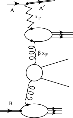
FIG. 4.: Diffractive hard scattering. A parton inside the pomeron undergoes a scattering scattering with a parton out of the antiproton.

E Relation between rapidity gaps and $x_{\mathbb{P}}$

Much diffractive data is presented as a function of the position of the edge of the pseudo-rapidity gap rather than as a function of $x_{\mathbb{P}}$. So it is useful to obtain an approximate relation between the two variables, in order to be able to compare different sets of data. I will present results both for the gaps in rapidity and in pseudo-rapidity.

1 Estimation of the size of the gap

In a typical event, the distribution of particles as a function of $y$ is supposed to look like Fig. 5(a). To estimate the relation between the edge of the rapidity gap and $x_{\mathbb{P}}$, I approximate the true distribution by a theta function distribution, Fig. 5(b). In the approximate distribution we have a uniform distribution, for values of $y$ less than a value I will call $y_{\rm edge}$, and no particles above $y_{\rm edge}$. The height of the distribution I will call $dN/dy$. From the distribution of hadrons in real diffractive events [4] I estimate that an appropriate value for $y_{\rm edge}$ is about one unit less than the actual end of the rapidity gap, in order to obtain the same value for $x_{\mathbb{P}}$.

(a)

(b)

FIG. 5.: (a) True distribution of particles in a diffractive event. (b) Theta-function approximation to this distribution.

Next, I split the computation of $x_{\mathbb{P}}$ into a sum over the high $p_{T}$ particles (e.g., associated with jets), and a sum over the low $p_{T}$ particles (which comprise what is often termed the ‘underlying event’). For the particles in the underlying event, I replace their transverse energy by its mean value $\langle E_{T}\rangle$. This gives

$$x_{\mathbb{P}} \simeq \beta_{\rm H}x_{\mathbb{P}}+\int_{-\infty}^{y_{\rm edge}}dy\,{\rm e}^{y}\,\frac{dN}{dy}\,\frac{\langle E_{T}\rangle}{2E}$$ (30)

$$= \beta_{\rm H}x_{\mathbb{P}}+{\rm e}^{y_{\rm edge}}\,\frac{dN}{dy}\,\frac{\langle E_{T}\rangle}{2E}.$$ (31)

Here, I have extended the integral over $y$ to $-\infty$, since, in the underlying event, only the hadrons closest to the edge of the rapidity gap are important in the calculation. Hence

$$\ln\frac{1}{x_{\mathbb{P}}} \simeq -\ln\frac{1}{1-\beta_{\rm H}}-y_{\rm edge}-\ln\frac{dN}{dy}+\ln\frac{2E}{\langle E_{T}\rangle}$$ (32)

$$= -y_{\rm max}-\ln\left(\frac{1}{1-\beta_{\rm H}}\right)+\left[\ln\frac{2E}{\langle E_{T}\rangle}+y_{\rm max}-y_{\rm edge}-\ln\frac{dN}{dy}\right],$$ (33)

with the term in square brackets being approximately independent of the event’s kinematic parameters, $y_{\rm max}$ and $\beta_{\rm H}$.

2 Numerical values

For a relation between $x_{\mathbb{P}}$ and the maximum measured pseudorapidity, let us rewrite Eq. (33) as

$$\ln\frac{1}{x_{\mathbb{P}}}=C-\eta_{\rm max}-\ln\frac{1}{1-\beta_{\rm H}}+\ln\frac{E}{900\,{\rm GeV}},$$ (34)

with

$$C=\eta_{\rm max}-y_{\rm edge}+\ln\frac{1800\,{\rm GeV}}{\langle E_{T}\rangle}-\ln\frac{dN}{dy}.$$ (35)

Now $C$ is a pure number that should be approximately independent of any of the parameters of the collision. So we can try to estimate it from the CDF data on single diffraction [4]. Their plots for the number distribution of charged tracks as a function of pseudo-rapidity are averaged over all events. Since different events have different values of $x_{\mathbb{P}}$, the plot need not exhibit a rapidity plateau even if individual events do so. Moreover the rise of $dN/dy$ from zero to its plateau will be spread out.

From the data, I estimate that at $\sqrt{s}=1800\,{\rm GeV}$

$$\frac{dN}{d\eta} \approx 2,$$ (36)

$$\eta_{\rm max}-y_{\rm edge} \approx 1.$$ (37)

In addition I use the value [6] $\langle E_{T}\rangle\approx 0.3\,{\rm GeV}$. These values give $C=8.5$.

Eq. (34) is, of course, not exact on an event-by-event basis. However, it should be useful on average, with the real data being smeared around the values related by the formula, and of course the numerical value ‘8.5’ should be adjusted by a fit to ordinary single diffraction data.

There is indeed such data. CDF in Ref. [7] give a plot of $\eta_{\rm max}$ against $x_{\mathbb{P}}$ for their diffractive dijet data. Unfortunately, it disagrees quite badly with the above formula, both as to normalization and slope. This needs to be investigated. For example, the numbers I quoted above in Eq. (37) may be wrong, and my formulae have made no allowance for the fact that the measured $\eta_{\rm max}$ applies to particles above some value of $E_{T}\approx 400\,{\rm MeV}$. The true $\eta_{\rm max}$ may be rather larger.

REFERENCES

- [1] H1 collaboration (T. Ahmed et al.), Nucl. Phys. B435, 2 (1995).
- [2] F. Jacquet and A. Blondel, in Proc. of the study for an facility in Europe, ed. U. Amaldi, DESY 79/48 (1979) pp. 391–394.
- [3] G. Ingelman and P. Schlein, Phys. Lett. 152B, 256 (1985).
- [4] CDF Collaboration (F. Abe et al.), Phys. Rev. D50, 5535 (1994).
- [5] CHLM Collaboration (M.G. Albrow et al.), Phys. Lett. 51B, 424 (1974).
- [6] CDF Collaboration (presented by M. Schub), “CDF Minimum Bias Results”, in Proceedings, Elastic and diffractive scattering Nucl. Phys. B, Proc. Suppl. 12 (1990) 254.
-
[7]
The relation between and in
diffractive jet production at CDF can be found in:
P.L. Mélèse for the CDF collaboration,
“Diffractive Dijet Search with Roman Pots at CDF”
FERMILAB-CONF-96-231-E, contributed to 1996 Annual Divisional
Meeting (DPF 96) of the Division of Particles and Fields of
the American Physical Society, Minneapolis, MN, 10–15 Aug. 1996,
http://www-lib.fnal.gov/archive/1996/conf/Conf-96-231-E.ps.
In that paper, is used to denote what I call .