Gauge Invariant Higgs mass bounds from the Physical Effective Potential

Abstract

We study a simplified version of the Standard Electroweak Model and introduce the concept of the physical gauge invariant effective potential in terms of matrix elements of the Hamiltonian in physical states. This procedure allows an unambiguous identification of the symmetry breaking order parameter and the resulting effective potential as the energy in a constrained state. We explicitly compute the physical effective potential at one loop order and improve it using the RG. This construction allows us to extract a reliable, gauge invariant bound on the Higgs mass by unambiguously obtaining the scale at which new physics should emerge to preclude vacuum instability. Comparison is made with popular gauge fixing procedures and an “error” estimate is provided between the Landau gauge fixed and the gauge invariant results.

I Introduction and Motivation

Considerable effort has been invested in understanding the Higgs sector of the Standard Model. Reliable constraints on the Higgs boson mass are important in determining the energy scales for collider experiments that probe the electroweak symmetry breaking sector. Alternately, should the Higgs be discovered, its properties will help elucidate high-scale physics. (see[1] for an early review). In the Standard Model the requirement that the conventional effective potential $V_{\rm{eff}}(\varphi)$ have its global minimum at the electroweak scale has been used to obtain a relation between a lower bound on the mass of the Higgs boson and the scale at which new physics should appear (for recent reviews see[2, 3]). That scale is related to the value of $\varphi$ (expectation value of the Higgs field) at which $V_{\rm{eff}}$ develops a new deeper minimum (which depends on the mass of the Higgs). Recently Loinaz and Willey[4] have pointed out a difficulty with this procedure. When the contributions from the gauge sector of the electroweak theory are included in the effective potential, the value of $\varphi$ which minimizes $V_{\rm{eff}}$ is gauge dependent. The gauge dependence of the effective potential was already recognized by Dolan and Jackiw in their early formulation of effective potentials[5]. Although in some specific gauges the contribution of the gauge sector may be a perturbative correction to the contributions from the scalar plus heavy (top) fermion-Yukawa sector, the gauge dependence implies that no error estimate can be made and raises questions on the reliability of such bounds. The conventional $V_{\rm{eff}}$, defined in terms of 1PI Green’s functions at zero momentum is an off-shell quantity and in a gauge-fixed formulation is inherently gauge variant and therefore not uniquely defined. Using the effective potential to study stability or metastability implicitly assumes that $V_{\rm{eff}}$ is associated with the energy of (space-time constant) field configurations. In scalar field theories the effective potential is proven to be the energy of a constrained state[6, 7, 8, 9], but such proof is lacking in gauge theories. Since the effective potential as calculated in gauge-fixed formulations is explicitly gauge dependent, it cannot generally be identified with the expectation value of the physical Hamiltonian in a physical state. There are, however, gauge independent quantities that can be extracted from the effective potential. Nielsen identities[10] have been used to prove that the difference of the values of the (gauge fixed) effective potential evaluated at extrema are gauge invariant, as well as the nucleation rate for bubbles in a first order transition when calculated from the effective potential[11]. However providing a lower bound on the Higgs mass requires to estimate values of the expectation value of the scalar order parameter, which is a gauge variant quantity even at the minima of the effective potential.

Thus it is important to provide a formulation in which the effective potential is a gauge invariant function of a gauge invariant order parameter and can be interpreted as an energy function. There have been efforts to formulate a gauge invariant effective action[12] and consequently an effective potential, but the formalism involved is formidable and its calculational implementability rather unwieldy.

Recently a formulation that allows to obtain a gauge invariant effective potential as the expectation value of the Hamiltonian in physical states has been developed within a different framework[13]. We refer to this as the Physical Effective Potential (PEP). In this article we apply the formulation proposed in[13] to solve the problem of the gauge dependence in a slight variant of the model studied in[4]. Although this model is a simplified Abelian version of the Standard Model, it serves to demonstrate the utility of the gauge-invariant effective potential in providing a gauge-invariant estimate of a vacuum instability scale.

This article is organized as follows: in section II we present the model to be studied and the relevant aspects of the gauge invariant formulation provided in[13] and adapted to include the fermionic sector. In this section we define the physical (gauge invariant) observables including the order parameter that provides an unambiguous signal for symmetry breaking. In section III we explicitly construct the one loop effective potential as the expectation value of the physical Hamiltonian in gauge invariant states constrained to give a space-time constant expectation value of the gauge invariant order parameter. We also provide the $\overline{\rm MS}$ renormalization of this effective potential. In section IV we compare our results to those obtained from the gauge fixed formulation in general $R_{\xi,u}$ gauges. Section V is devoted to a RG improvement of the gauge invariant effective potential and to an unambiguous determination of the lower bound on the Higgs mass in this model, providing “error estimates” for the quantities obtained in the gauge variant formulation. In Section VI we present some brief numerical results.

Section VII summarizes our conclusions and suggests possibles avenues to extend the gauge invariant construction to non-Abelian gauge theories.

II The Gauge Invariant Description:

The focus of our study is the Abelian Higgs model with an axial coupling of the gauge fields to fermions. The Lagrangian density is

$${\cal{L}} = -\frac{1}{4}F^{\mu\nu}F_{\mu\nu}+D^{\mu}\phi^{\dagger}D_{\mu}\phi-\mu^{2}\phi^{\dagger}\phi-\lambda(\phi^{\dagger}\phi)^{2}+\bar{\psi}\left[i{D\!\!\!\!/}+y\left(\phi_{1}+i\gamma^{5}\phi_{2}\right)\psi\right]$$ (1)

$$D_{\mu}\phi = (\partial_{\mu}\phi+ieA_{\mu}\phi)\;;\;{D\!\!\!\!/}=\gamma^{\mu}\left(\partial_{\mu}-ie\gamma^{5}\frac{A_{\mu}}{2}\right)\;;\;\phi=\frac{1}{\sqrt{2}}\left(\phi_{1}+i\phi_{2}\right)$$ (2)

Our goal is to define and explicitly evaluate the gauge invariant effective potential, in terms of a gauge invariant order parameter. The definition of the effective potential that we use is in terms of the expectation value of the physical Hamiltonian in physical states constrained to provide a fixed expectation value of the physical order parameter.

The program for the construction of such an effective potential requires i) the identification of the physical (gauge invariant) states of the theory, ii) the identification of an order parameter that is invariant under the local gauge transformation but transforms nontrivially under the rigid global symmetry transformation and thus gives information on spontaneous symmetry breaking iii) construction of the gauge invariant effective potential as the expectation value of the Hamiltonian in constrained physical states. Since the concepts behind the construction are not part of the standard lore, we highlight below the most relevant aspects of the formulation, for more details see[13].

Such a description is best achieved within the canonical formulation, which begins with the identification of canonical field variables and constraints. These will determine the classical physical phase space and, at the quantum level, the physical Hilbert space.

The canonical momenta conjugate to the scalar and vector fields are given by

$$\Pi^{0} = 0\;;\;\Pi^{i}=\dot{A}^{i}+\nabla^{i}A^{0}=-E^{i}$$ (3)

$$\pi^{\dagger} = \dot{\phi}+ieA^{0}\phi\;;\;\pi=\dot{\phi}^{\dagger}-ieA^{0}\phi^{\dagger}$$ (4)

The Hamiltonian is therefore

$$H= \int d^{3}x\left\{\frac{1}{2}\vec{\Pi}\cdot\vec{\Pi}+\pi^{\dagger}\pi+(\vec{\nabla}\phi-ie\vec{A}\phi)\cdot(\vec{\nabla}\phi^{\dagger}+ie\vec{A}\phi^{\dagger})+\frac{1}{2}(\vec{\nabla}\times\vec{A})^{2}+\right.$$ (7)

$$\left.\mu\phi^{\dagger}\phi+\lambda(\phi^{\dagger}\phi)^{2}+A_{0}\left[\vec{\nabla}\cdot\vec{\Pi}-ie(\pi\phi-\pi^{\dagger}\phi^{\dagger})+i\frac{e}{2}\psi^{\dagger}\gamma^{5}\psi\right]+\right.$$

$$\left.\psi^{\dagger}\left[-i\vec{\alpha}\cdot\left(\vec{\nabla}-i\frac{e}{2}\gamma^{5}\vec{A}\right)+\beta y\left(\phi_{1}+i\gamma^{5}\phi_{2}\right)\right]\psi\right\}$$

where $\vec{\alpha}\;;\beta$ are the Dirac matrices.

There are two main methods for quantizing gauge theories, the first one originally due to Dirac[14](see also[15]) begins by identifying the first class (mutually commuting) constraints and projects the physical states by requiring that these are simultaneously annihilated by all first class constraints. Physical operators commute with all of the first class constraints. The second, and most used method, “fixes a gauge”, converting the set of first class constraints into second class constraints (non-commuting) and introducing the Dirac brackets. This is the popular method of dealing with the constraints and leads to the usual gauge-fixed path integral representation[16] in terms of Faddeev-Popov determinants and ghosts. Although this second method is the most popular as it is easily translated into a path integral language, it has the drawback that the physical quantities are more difficult to extract, and though S-matrix elements are gauge invariant, off-shell quantities generally are not.

In order to avoid ambiguities and to define a physical order parameter and effective potential (an off-shell quantity) we choose to use the first method.

In Dirac’s method of quantization[14, 15] there are two first class constraints which are:

$$\Pi^{0}=\frac{\delta{\cal{L}}}{\delta A^{0}}=0$$ (8)

and Gauss’ law:

$${\cal{G}}(\vec{x},t) = \vec{\nabla}\cdot\vec{\Pi}-\rho=0$$ (9)

$$\rho = \left[ie(\pi\phi-\pi^{\dagger}\phi^{\dagger})-i\frac{e}{2}\psi^{\dagger}\gamma^{5}\psi\right]$$ (10)

with $\rho$ being the matter (complex scalar and fermionic) field charge density.

Gauss’ law can be seen to be a constraint in two ways: either because it cannot be obtained as a Hamiltonian equation of motion, or because in Dirac’s formalism, it is the secondary (first class) constraint obtained by requiring that the primary constraint (8) remain constant in time. Quantization is now achieved by imposing the canonical equal-time commutation relations

$$\left[\Pi^{0}(\vec{x},t),A^{0}(\vec{y},t)\right]=-i\delta(\vec{x}-\vec{y})\;\;;\;\;\left[\Pi^{i}(\vec{x},t),A^{j}(\vec{y},t)\right]=-i\delta^{ij}\delta(\vec{x}-\vec{y})\\$$ (11)

along with the usual canonical commutators for the scalar field and its canonical momentum and anticommutators for the fermionic fields.

In Dirac’s formulation, the projection onto the gauge invariant subspace of the full Hilbert space is achieved by imposing the first class constraints onto the states. Physical operators are those that commute with the first class constraints. Since $\Pi^{0}(\vec{x},t)$ and ${\cal{G}}(\vec{x},t)$ are generators of local gauge transformations, operators that commute with the first class constraints are gauge invariant[13].

Following the steps of reference[13] we find that the fields and canonical conjugate momenta

$$\Phi(\vec{x}) = \phi(\vec{x})\exp\left[ie\int d^{3}y\vec{A}(\vec{y})\cdot\vec{\nabla}_{y}G(\vec{y}-\vec{x})\right]=\frac{1}{\sqrt{2}}\left(\Phi_{1}+i\Phi_{2}\right)$$ (12)

$$\Pi(\vec{x}) = \pi(\vec{x})\exp\left[-ie\int d^{3}y\vec{A}(\vec{y})\cdot\vec{\nabla}_{y}G(\vec{y}-\vec{x})\right]$$ (13)

$$\Psi(\vec{x}) = \exp\left[-i\frac{e}{2}\gamma^{5}\int d^{3}y\vec{A}(\vec{y})\cdot\vec{\nabla}_{y}G(\vec{y}-\vec{x})\right]\psi(\vec{x})$$ (14)

with $G(\vec{y}-\vec{x})$ the Coulomb Green’s function that satisfies

$$\nabla^{2}G(\vec{y}-\vec{x})=\delta^{3}(\vec{y}-\vec{x})$$ (15)

are invariant under the gauge transformations[13]. Furthermore writing the gauge field into transverse and longitudinal components as follows

$$\vec{A}(\vec{x})=\vec{A}_{L}(\vec{x})+\vec{A}_{T}(\vec{x})$$ (16)

$$\vec{\nabla}\times\vec{A}_{L}(\vec{x})=0\;\;;\;\;\vec{\nabla}\cdot\vec{A}_{T}(\vec{x})=0$$ (17)

it is clear that the “transverse component” $\vec{A}_{T}(\vec{x})$ is also a gauge invariant operator. The fields $\vec{A}_{T}\;;\Phi\;;\Psi$ and their canonical momenta are gauge invariant as they commute with the constraints. The momentum canonical to $\vec{A}\;;\;\vec{\Pi}$ is written in terms of “longitudinal” and “transverse” components

$$\vec{\Pi}(\vec{x})=\vec{\Pi}_{L}(\vec{x})+\vec{\Pi}_{T}(\vec{x}).$$ (18)

Both components are gauge invariant.

In the physical subspace of gauge invariant wave-functionals, matrix elements of $\vec{\nabla}\cdot\vec{\Pi}$ can be replaced by matrix elements of the charge density $\rho$, since matrix elements of Gauss’ law between these states vanish. Therefore in all matrix elements between gauge invariant states (or functionals) one can replace

$$\vec{\Pi}_{L}(\vec{x})\rightarrow\rho$$ (19)

with the charge density (a gauge invariant operator) written in terms of the gauge invariant fields as

$$\rho=\left[ie\left(\Phi(\vec{y})\Pi(\vec{y})-\Phi^{\dagger}(\vec{y})\Pi^{\dagger}(\vec{y})\right)-i\frac{e}{2}\Psi^{\dagger}(\vec{y})\gamma^{5}\Psi(\vec{y})\right]$$ (20)

This procedure is tantamount to solving the constraints in the physical space[15].

Finally in the gauge invariant subspace the Hamiltonian becomes

$$H= \int d^{3}x\left\{\frac{1}{2}\vec{\Pi}_{T}\cdot\vec{\Pi}_{T}+\Pi^{\dagger}\Pi+(\vec{\nabla}\Phi-ie\vec{A}_{T}\Phi)\cdot(\vec{\nabla}\Phi^{\dagger}+ie\vec{A}_{T}\Phi^{\dagger})+\frac{1}{2}(\vec{\nabla}\times\vec{A}_{T})^{2}+\right.$$ (23)

$$\left.\mu^{2}\Phi^{\dagger}\Phi+\lambda(\Phi^{\dagger}\Phi)^{2}+\Psi^{\dagger}\left[-i\vec{\alpha}\cdot\left(\vec{\nabla}-i\frac{e}{2}\gamma^{5}\vec{A}_{T}\right)+\beta y\left(\Phi_{1}+i\gamma^{5}\Phi_{2}\right)\right]\Psi\right\}+$$

$$\frac{1}{2}\int d^{3}y\int d^{3}x\rho(\vec{x})G(\vec{x}-\vec{y})\rho(y)$$

Clearly the Hamiltonian is gauge invariant, and it manifestly has the global $U(1)$ (chiral) symmetry under which

$$\Phi(\vec{x})\rightarrow\Phi(\vec{x})e^{i\varphi}\;\;;\;\;\Psi(\vec{x})\rightarrow e^{-i\gamma^{5}\frac{\varphi}{2}}\Psi(\vec{x})$$ (24)

with $\varphi$ a constant real phase, $\Pi$ transforms with the opposite phase and $\vec{A}_{T}$ is invariant.

The Hamiltonian written in terms of gauge invariant field operators (23) is reminiscent of the Coulomb gauge Hamiltonian, but we emphasize that we have not imposed any gauge fixing condition. The formulation is fully gauge invariant, written in terms of operators that commute with the generators of gauge transformations and states that are invariant under these transformations. The similarity to the Coulomb gauge Hamiltonian is a consequence of the fact that in this Abelian theory, Coulomb gauge displays explicitly the physical degrees of freedom.

There is a definite advantage in this gauge invariant formulation: the (composite) field $\Phi(\vec{x})$ is a candidate for a locally gauge invariant order parameter. The point to stress is the following: this operator is invariant under local gauge transformations but it transforms as a charged operator under the global gauge transformations generated by $Q=\int d^{3}x\rho(\vec{x})$, that is

$$e^{i\alpha Q}\Phi(\vec{x})e^{-i\alpha Q}=e^{ie\alpha}\Phi(\vec{x}).$$ (25)

Because the gauge constraints annihilate the physical states and these constraints are the generators of local gauge transformations[13, 15], these states are invariant under the local gauge transformations and any operator that is not invariant under these local transformations must have zero expectation value. The local gauge symmetry cannot be spontaneously broken; this result is widely known in lattice gauge theory as Elitzur’s theorem[18]. However, the global symmetry generated by the charge $Q$ can be spontaneously broken and the expectation value of a charged field signals this breakdown.

From this discussion we clearly see that a trustworthy order parameter must be invariant under the local gauge transformations, thus commuting with the gauge constraints, but must transform non-trivially under the global gauge transformation generated by the charge. The field $\Phi$ fulfills these criteria and is the natural candidate for an order parameter.

At this stage, having recognized the physical states one could prefer to pass to a path integral representation of the vacuum-in to vacuum-out transition amplitude. This can now be done unambiguously by carrying out the usual procedure in terms of phase space path integrals with the gauge invariant measure ${\cal{D}}\vec{\Pi}_{T}{\cal{D}}{\vec{A}}_{T}{\cal{D}}\Phi{\cal{D}}\Phi^{\dagger}{\cal{D}}\Pi{\cal{D}}\Pi^{\dagger}\cdots$. There is no need for “gauge fixing”. In the resulting action (of the form $p\dot{q}-H$), the instantaneous Coulomb interaction can be re-written by introducing an auxiliary field, and the integral over the canonical momenta can be carried out explicitly leading to a Lagrangian form. The resulting Lagrangian leads to Feynman rules that are very similar to those in Coulomb gauge and allow the perturbative calculation of wave function renormalization constants needed below. The gauge invariant effective potential can also be computed in this path integral representation, but we prefer to provide its explicit construction from the Hamiltonian as such construction displays more clearly the identification of the effective potential as the energy of a constrained state.

III The Effective Potential

We are now in position to define the gauge invariant effective potential. Consider the class of gauge invariant states $|\Upsilon,\chi\rangle$ characterized by the condition that the expectation value of the gauge invariant order parameter $\Phi(\vec{x})$ in this state is nonzero and space-time constant

$$\frac{\langle\Upsilon,\chi|\Phi(\vec{x})|\Upsilon,\chi\rangle}{\langle\Upsilon,\chi|\Upsilon,\chi\rangle}=\frac{1}{\sqrt{2}}(\chi_{1}+i\chi_{2})\equiv\chi$$ (26)

In this notation $\Upsilon$ indexes the states within the set characterized by eq. 26. The effective potential is defined as the minimum of the expectation value of the Hamiltonian density over this class of constrained states [6, 7, 8], namely

$$V_{\rm{eff}}(\chi)=\frac{1}{\Omega}\min_{\Upsilon}\left\{\frac{\langle\Upsilon,\chi|H|\Upsilon,\chi\rangle}{\langle\Upsilon,\chi|\Upsilon,\chi\rangle}\right\}$$ (27)

with $H$ being the gauge invariant Hamiltonian given by equation (23) and $\Omega$ the spatial volume[9]. By construction in terms of gauge invariant states (or functionals) and the gauge invariant Hamiltonian, this effective potential is gauge invariant. The minima of this effective potential are obtained from $V_{\rm{eff}}(\chi)$ by further minimizing with respect to $\chi_{1,2}$.

It is convenient to separate the expectation value of $\Phi$ as

$$\Phi(\vec{x}) = \frac{1}{\sqrt{2}}(\chi_{1}+i\chi_{2})+\frac{1}{\sqrt{2}}(\eta_{1}(\vec{x})+i\eta_{2}(\vec{x}))$$ (28)

$$\Pi(\vec{x}) = \frac{1}{\sqrt{2}}(\Pi_{1}(\vec{x})-i\Pi_{2}(\vec{x}))$$ (29)

The one-loop correction (formally of ${\cal{O}}(\hbar)$) to the effective potential is obtained by keeping the linear and quadratic terms in $\eta_{1,2}$ in the Hamiltonian, however the linear terms will not contribute to the effective potential because their contribution vanishes upon taking the expectation value in the state $|\Upsilon,\chi\rangle$. Thus keeping only the quadratic terms in $\eta_{1,2}$ we obtain

$$H_{q} = \Omega\left(\frac{\mu^{2}}{2}|\chi|^{2}+\frac{\lambda}{4}|\chi|^{4}\right)+H_{q}^{B}+H^{F}$$ (30)

$$H_{q}^{B} = \frac{1}{2}\int d^{3}x\left\{\vec{\Pi}^{2}_{T}+(\vec{\nabla}\times\vec{A})^{2}+e^{2}|\chi|^{2}\vec{A}^{2}_{T}+\Pi^{2}_{1}+\Pi^{2}_{2}+(\vec{\nabla}\eta_{1})^{2}+(\vec{\nabla}\eta_{2})^{2}+\right.$$ (32)

$$\left.\eta^{2}_{1}(\mu^{2}+3\lambda|\chi|^{2})+\eta^{2}_{2}(\mu^{2}+\lambda|\chi|^{2})\right\}-\frac{e^{2}}{2}|\chi|^{2}\int d^{3}x\int d^{3}y\Pi_{2}(\vec{x})G(\vec{x}-\vec{y})\Pi_{2}(\vec{y})$$

$$H^{F} = \int d^{3}x\left\{\Psi^{\dagger}\left[-i\vec{\alpha}\cdot\nabla+y|\chi|\beta\right]\Psi\right\}$$ (33)

where we have performed a rigid chiral phase rotation under which the Hamiltonian is invariant. The transverse components $\vec{A}_{T}$ describe a field with mass $m_{T}^{2}=e^{2}|\chi|^{2}$ and only two polarizations. The fermionic part is recognized as a free Dirac fermion with mass $M_{F}=y|\chi|$. The fermionic Hamiltonian can be diagonalized in terms of particle and antiparticle creation and annihilation operators of the usual form, and upon using their anticommutation relation we obtain

$$H^{F} = \sum_{k}\sum_{a=1,2}\left\{\omega^{F}(k)\left[b^{\dagger}_{k,a}b_{k,a}+d^{\dagger}_{k,a}d_{k,a}\right]\right\}-2\sum_{k}\omega^{F}(k)$$ (34)

$$\omega^{F}(k) = \sqrt{k^{2}+M^{2}_{F}[|\chi|]}\;\;;\;\;M_{F}[\chi]=y|\chi|$$ (35)

Following[13] we write the bosonic Hamiltonian ($H_{q}^{B}$) in terms of the spatial Fourier transform of the fields and their canonical momenta in terms of which the quadratic part of the Hamiltonian finally becomes

$$H_{q} = \Omega V_{cl}(|\chi|)+\frac{1}{2}\sum_{k}\left\{\vec{\Pi}_{T}(k)\cdot\vec{\Pi}_{T}(-k)+\omega^{2}_{T}(k)\vec{A}_{T}(k)\cdot\vec{A}_{T}(-k)+\right.$$ (37)

$$\left.\Pi_{1}(k)\Pi_{1}(-k)+\omega^{2}_{H}(k)\eta_{1}(k)\eta_{1}(-k)+\Pi_{2}(k)\Pi_{2}(-k)\frac{\omega^{2}_{T}(k)}{k^{2}}+\eta_{2}(k)\eta_{2}(-k)\omega^{2}_{g}(k)\right\}$$

where the frequencies are given in terms of the effective masses as

$$\omega^{2}_{T}(k)=k^{2}+M^{2}_{T}[\chi] \;\;;\;\; M^{2}_{T}[\chi]=e^{2}|\chi|^{2}$$ (38)

$$\omega^{2}_{H}(k)=k^{2}+M^{2}_{H}[\chi] \;\;;\;\; M^{2}_{H}[\chi]=\mu^{2}+3\lambda|\chi|^{2}$$ (39)

$$\omega^{2}_{g}(k)=k^{2}+M^{2}_{g}[\chi] \;\;;\;\; M^{2}_{g}[\chi]=\mu^{2}+\lambda|\chi|^{2}.$$ (40)

The last two terms can be brought to a canonical form by a Bogoliubov transformation. Define the new canonical coordinate $Q$ and conjugate momentum $P$ as

$$\Pi_{2}(k)=\frac{k}{\omega_{T}(k)}P(k)\;\;;\;\;\eta_{2}(k)=\frac{\omega_{T}(k)}{k}Q(k)$$ (41)

in terms of which the last term of the Hamiltonian (37) becomes a canonical quadratic form with the plasma frequency

$$\omega^{2}_{p}(k)=\omega^{2}_{g}(k)\frac{\omega^{2}_{T}(k)}{k^{2}}=[k^{2}+M^{2}_{g}[\chi]][k^{2}+M^{2}_{T}[\chi]]/k^{2}$$ (42)

There are four physical degrees of freedom. The modes with frequency $\omega_{T}(k)$ are the two transverse degrees of freedom, the mode with frequency $\omega_{H}(k)$ is identified with the Higgs mode. In absence of electromagnetic interactions ($e=0$) the mode with frequency $\omega_{p}(k)$ represents the Goldstone mode whereas in equilibrium, namely at the minimum of the tree level potential, when $|\chi|=\sqrt{-\mu^{2}/\lambda}$, it represents the plasma mode which is identified as the screened Coulomb interaction, and the transverse and plasma modes all share the same mass. A detailed discussion of the dispersion relation of the bosonic excitations has been provided in[13].

The quadratic Hamiltonian is now diagonalized in terms of creation and destruction operators for the quanta of each harmonic oscillator. The ground state is the vacuum for each oscillator and is the state of lowest energy compatible with the constraint (26). Therefore the one loop (${\cal{O}}(\hbar)$) contribution to the effective potential is obtained from the zero point energy of the bosonic oscillators and the (negative) contribution from the “Dirac sea” given by the last term in (34). Therefore accounting for the two polarizations of the transverse components we find:

$$V_{\rm{eff}}(|\chi|)=V_{cl}(|\chi|)+\frac{1}{2}\int\frac{d^{3}k}{(2\pi^{3})}[2\omega_{T}(k)+\omega_{H}(k)+\omega_{p}(k)-4\omega^{F}(k)]$$ (43)

The normalized state that satisfies (26) and gives the minimum expectation value of the Hamiltonian, thus determining effective potential via (27) is given by

$$|\chi\rangle=|\chi\rangle_{T_{1}}\otimes|\chi\rangle_{T_{2}}\otimes|\chi\rangle_{H}\otimes|\chi\rangle_{p}\otimes|\chi\rangle_{F}$$ (44)

i.e. a tensor product of the harmonic oscillator ground states for the two polarizations ( $T_{1,2}$ ), the Higgs mode (H), the “plasma” mode (p) and the fermionic Fock state (F) (the “Dirac sea”). The functional representation for the bosonic Fock states is simply a Gaussian wave-functional. This state by construction is gauge invariant.

The k-integrals in the final form of the gauge invariant effective potential (43) are carried out in dimensional regularization by the replacements: $\int d^{3}k/(2\pi)^{3}\rightarrow\int d^{d-1}k/(2\pi)^{d-1};g_{\mu}^{\mu}=d$, and $2\rightarrow d-2$ transverse modes, $d=4-\epsilon$ (see the appendix) and we obtain the following (unrenormalized expression) one loop effective potential

$$V_{\rm{eff}}(\chi)=V_{cl}(\chi) + \frac{1}{(4\pi)^{2}}\left\{-\Delta_{\epsilon}\left[\frac{M^{4}_{T}[\chi]}{2}+\frac{M^{4}_{H}[\chi]}{4}+\frac{1}{4}(M^{2}_{T}[\chi]-M^{2}_{g}[\chi])^{2}-M^{4}_{F}[\chi]\right]+\right.$$ (48)

$$\left.\frac{M^{4}_{T}[\chi]}{2}\left(\ln\left[\frac{M^{2}_{T}[\chi]}{\kappa^{2}}\right]-\frac{1}{2}\right)+\frac{M^{4}_{H}[\chi]}{4}\left(\ln\left[\frac{M^{2}_{H}[\chi]}{\kappa^{2}}\right]-\frac{3}{2}\right)+\right.$$

$$\left.\frac{1}{4}\left(M^{2}_{T}[\chi]-M^{2}_{g}[\chi][\chi]\right)^{2}\left(\ln\left[\frac{(M_{T}[\chi]+M_{g}[\chi])^{2}}{\kappa^{2}}\right]-\frac{3}{2}\right)\right.$$

$$\left.-\frac{1}{2}M_{T}[\chi]M_{g}[\chi](M_{T}[\chi]-M_{g}[\chi])^{2}-M^{4}_{F}[\chi]\left(\ln\left[\frac{M^{2}_{F}[\chi]}{\kappa^{2}}\right]-\frac{3}{2}\right)\right\}$$

with

$$\Delta_{\epsilon}=\frac{2}{4-d}-\gamma+\ln[4\pi]$$ (49)

is the standard $\overline{\rm MS}$ UV subtraction in d-dimensions, $\kappa$ is the renormalization scale and $\gamma$ is the Euler-Mascheroni constant.

A $\overline{\rm MS}$ Renormalization

The theory is renormalized by coupling, mass and wavefunction renormalizations.

$$e_{b}=Z_{e}e_{R}\;;\;\lambda_{b}=Z_{\lambda}\lambda_{R}\;;\;y_{b}=Z_{y}y_{R}\;;\;\mu^{2}_{b}=Z_{\mu^{2}}\mu^{2}_{R}$$ (50)

$$A^{\mu}_{b}=Z^{\frac{1}{2}}_{A}A_{R}\;;\;\Phi_{b}=Z^{\frac{1}{2}}_{\Phi}\Phi_{R}\;;\;\Psi_{b}=Z^{\frac{1}{2}}_{\Psi}\Psi_{R}$$ (51)

The gauge invariant quantization ensures that all the Ward identities associated with the gauge symmetry are now trivially satisfied. Here we work in the $\overline{\rm MS}$ renormalization scheme and write for the various couplings and wavefunction renormalizations $Z=1+\delta Z$, expanding $\delta Z$ in powers of the couplings and absorbing only the $\overline{\rm MS}$ divergences proportional to $\Delta_{\epsilon}$. There are two equivalent procedures to renormalize the effective potential:

1. The terms proportional to $\Delta_{\epsilon}$ in (48) are absorbed in a partial renormalization of couplings and $\mu^{2}$. This renormalization, however, does not render finite the scattering amplitudes. The latter require a further renormalization by the proper wave function renormalization constants, which at the level of the effective potential is absorbed in a renormalization of $\chi^{2}_{b}\rightarrow Z_{\Phi}\chi^{2}_{R}$. The wave-function renormalizations must be calculated differently from the effective potential, since their calculation requires one-loop contributions at non-zero momentum.

2. After restricting the Hamiltonian to the gauge invariant subspace, one can pass on to the Lagrangian density in terms of gauge invariant variables, and write it in terms of the renormalized couplings, masses and fields plus the counterterm Lagrangian. The counterterms are then required to cancel the divergences in the proper 1PI Green’s functions. It is at this stage that we use the path integral representation discussed previously to compute the wave function renormalization constants from the one loop self-energies and vertex corrections. Such a calculation, although straightforward, involves non-covariant loop integrals which are performed with the help of the appendix in reference[19].

For the renormalization of the effective potential only scalar wave function renormalization is needed beyond the cancellation of the terms proportional to $\Delta_{\epsilon}$ in (48). A lengthy but straightforward calculation of the relevant one loop diagrams provides the renormalization constants listed in Appendix B.

In terms of the renormalized couplings and expectation value of the gauge invariant scalar field, the gauge invariant effective potential in the $\overline{\rm MS}$ renormalization scheme is given by (here we drop the subscripts (R) in the renormalized quantities to avoid cluttering of notation, but all quantities below are renormalized)

$$V_{\rm{eff}}(\chi) = V_{cl}(\chi)+\frac{1}{(4\pi)^{2}}\left\{\frac{M^{4}_{T}[\chi]}{2}\left(\ln\left[\frac{M^{2}_{T}[\chi]}{\kappa^{2}}\right]-\frac{1}{2}\right)+\frac{M^{4}_{H}[\chi]}{4}\left(\ln\left[\frac{M^{2}_{H}[\chi]}{\kappa^{2}}\right]-\frac{3}{2}\right)+\right.$$ (54)

$$\left.\frac{1}{4}\left(M^{2}_{T}[\chi]-M^{2}_{g}[\chi]\right)^{2}\left(\ln\left[\frac{(M_{T}[\chi]+M_{g}[\chi])^{2}}{\kappa^{2}}\right]-\frac{3}{2}\right)\right.$$

$$\left.-\frac{1}{2}M_{T}[\chi]M_{g}[\chi](M_{T}[\chi]-M_{g}[\chi])^{2}-M^{4}_{F}[\chi]\left(\ln\left[\frac{M^{2}_{F}[\chi]}{\kappa^{2}}\right]-\frac{3}{2}\right)\right\}$$

IV Comparison with gauge-fixed results:

A comparison with the effective potential in covariant $R_{\xi,u}$ gauges is established by adding a gauge fixing and Faddeev-Popov terms to the Lagrangian density eq.(1):

$${\cal{L}}\rightarrow{\cal{L}}+{\cal{L}}_{gf}+{\cal{L}}_{FP}$$ (55)

$${\cal{L}}_{gf}=-\frac{1}{2\xi}(\partial_{\mu}A^{\mu}+\xi ue\phi_{2})^{2}$$ (56)

$${\cal{L}}_{FP}=-\bar{c}{\partial^{2}}c-\xi ue^{2}\bar{c}c\phi_{1}$$ (57)

Special cases of this covariant gauge fixing procedure include the Landau gauges $\left(\xi=0\right)$, ’t Hooft $R_{\xi}$ gauges [20] ($u=\left\langle\phi_{1}\right\rangle_{0}$, the tree-level Higgs $vev$) and Fermi gauges $\left(u=0\right)$ where we have chosen the symmetry breaking expectation value along the $\phi_{1}$ direction for convenience. At this stage we can just quote the results of reference[4] adapted to the case treated here of an axial vector coupling with $N_{f}=1$, for arbitrary number of flavors, the one-loop contribution from the fermion will be multiplied by $N_{f}$. With $\varphi=\langle\phi_{1}\rangle$ the expectation value obtained in the gauge-fixed path integral, we obtain the one loop effective potential in the $\overline{\rm MS}$ scheme after renormalization of $\mu^{2}$, couplings and wavefunctions[4]:

$$\tilde{V}_{eff}\left[\varphi;\xi;u\right] = {1\over 2}\mu^{2}\varphi^{2}+{{\lambda}\over 4}\varphi^{4}+{1\over 4}{{H^{4}\left[\varphi\right]}\over{\left(4\pi\right)^{2}}}\left[\ln{{{H^{2}\left[\varphi\right]}\over{\kappa^{2}}}}-{3\over 2}\right]$$ (61)

$$+{3\over 4}{{B^{4}\left[\varphi\right]}\over{\left(4\pi\right)^{2}}}\left[\ln{{{B^{2}\left[\varphi\right]}\over{\kappa^{2}}}}-{5\over 6}\right]-{2\over 4}{{G^{4}\left[\varphi\right]}\over{\left(4\pi\right)^{2}}}\left[\ln{{{G^{2}\left[\varphi\right]}\over{\kappa^{2}}}}-{3\over 2}\right]$$

$$+{1\over 4}{{k_{+}^{4}\left[\varphi\right]}\over{\left(4\pi\right)^{2}}}\left[\ln{{{k_{+}^{2}\left[\varphi\right]}\over{\kappa^{2}}}}-{3\over 2}\right]+{1\over 4}{{k_{-}^{4}\left[\varphi\right]}\over{\left(4\pi\right)^{2}}}\left[\ln{{{k_{-}^{2}\left[\varphi\right]}\over{\kappa^{2}}}}-{3\over 2}\right]$$

$$-{{Y^{4}\left[\varphi\right]}\over{\left(4\pi\right)^{2}}}\left[\ln{{{Y^{2}\left[\varphi\right]}\over{\kappa^{2}}}}-{3\over 2}\right]+\xi e^{2}u\varphi\left(\mu^{2}+\lambda\varphi^{2}\right)\left[\frac{-\Delta_{\epsilon}}{(4\pi)^{2}}\right]$$

where

$$H^{2}\left[\varphi\right] = \mu^{2}+3\lambda\varphi^{2}$$ (62)

$$B^{2}\left[\varphi\right] = e^{2}\varphi^{2}$$ (63)

$$G^{2}\left[\varphi\right] = \xi e^{2}u\varphi$$ (64)

$$k_{\pm}^{2}\left[\varphi\right] = {1\over 2}\left[\mu^{2}+\lambda\varphi^{2}+2\xi e^{2}u\varphi\right]\pm$$ (66)

$${1\over 2}\sqrt{\left(\mu^{2}+\lambda\varphi^{2}\right)\left(\mu^{2}+\lambda\varphi^{2}+4\xi e^{2}\varphi\left(u-\varphi\right)\right)}$$

$$Y^{2}\left[\varphi\right] = y^{2}\varphi^{2}$$ (67)

$H$, $B$, $Y$ and $G$ denote contributions from Higgs, vector boson, fermion and Fadeev-Popov ghost loops, respectively.

Although the “effective masses” $H[\varphi]\;;\;B[\varphi]\;;\;Y[\varphi]$ are formally similar to the Higgs, transverse and fermion effective masses given in equations (35,38,39) upon the replacement $\varphi\rightarrow|\chi|$, we want to emphasize that $\varphi_{\rm ex}$ is the expectation value of a gauge dependent field in a gauge-fixed state, whereas $\chi$ is a true gauge invariant order parameter, the expectation value of a gauge invariant field in a gauge invariant state. The UV pole in the gauge-fixed effective potential (61) which is not removed by couplings and wave-function renormalizations has been discussed in detail in[4]. It can be removed by a shift in $\varphi$ consistently in the loop expansion and is a consequence of the particular choice of $R_{\xi,u}$ gauge-fixing that breaks the global $U(1)$ symmetry explicitly.

Even for the Landau gauge, corresponding to the choice $\xi=0$, leading to $k_{+}^{2}=\mu^{2}+\lambda\varphi^{2};\;k_{-}^{2}=0$ the difference of the gauge sector contributions to the gauge fixed and the gauge invariant effective potential is clear.

The first physical quantity that we must compare is the value of both the gauge invariant and the gauge fixed effective potentials at their respective minima. The minima are obtained from the conditions

$$\left[{{\partial V_{\rm{eff}}\left[|\chi|\right]}\over{\partial|\chi|}}\right]\;\;;\;\;\left[{{\partial\tilde{V}_{eff}\left[\varphi;\xi;u\right]}\over{\partial\varphi}}\right]=0$$ (68)

Writing the stationary values of $|\chi|\;;\;\varphi$ in a formal loop expansion as[4]

$$|\chi|_{\rm ext}=|\chi|_{0}+|\chi|_{1}+\cdots\;;\;\varphi_{\rm ext}=\varphi_{0}+\varphi_{1}+\cdots$$ (69)

we find the following relations that fix the minima to one-loop order

$$0 = \left[{{\partial V^{0}_{eff}\left[|\chi|\right]}\over{\partial|\chi|}}\right]_{|\chi|_{0}}$$ (70)

$$|\chi|_{1} = -\left[{{\partial V^{1}_{eff}\left[|\chi|\right]}\over{\partial|\chi|}}\right]_{|\chi|_{0}}\left\{\left[{{\partial^{2}V^{0}_{eff}\left[|\chi|\right]}\over{\partial|\chi|^{2}}}\right]_{|\chi|_{0}}\right\}^{-1}$$ (71)

$$0 = \left[{{\partial\tilde{V}^{0}_{eff}\left[\varphi;\xi;u\right]}\over{\partial\varphi}}\right]_{\varphi_{0}}$$ (72)

$$\varphi_{1}(\xi;u) = -\left[{{\partial\tilde{V}^{1}_{eff}\left[\varphi;\xi;u\right]}\over{\partial\varphi}}\right]_{\varphi_{0}}\left\{\left[{{\partial^{2}\tilde{V}^{0}_{eff}\left[\varphi;\xi;u\right]}\over{\partial\varphi^{2}}}\right]_{\varphi_{0}}\right\}^{-1}$$ (73)

the solutions of eq.(70,72) are obviously the tree level vacuum expectation values $|\chi|_{0}=\varphi_{0}=\sqrt{-\mu^{2}/\lambda}$ but the solution of eq.(73) is dependent on the gauge fixing parameters $\xi,u$[4]. However, upon inserting the solutions of the minima equation consistently up to one loop in the respective expressions for the effective potentials, we find that the value of the minima for the gauge-fixed and the gauge invariant effective potential are the same. This is an important result: whereas the gauge invariant effective potential as constructed has the meaning of an energy of constrained physical states, no such interpretation is available for the gauge-fixed result. However at the minimum, we see that the gauge-fixed effective potential agrees with the gauge invariant result and therefore the values of the extrema provide gauge invariant information on the energetics of constrained states.

The second derivative of the gauge fixed effective potential at the minimum is seen to be a gauge dependent quantity. Although the pole mass of the excitations are on-shell quantities and must therefore be gauge invariant, the second derivative of the effective potential corresponds to the value of the one-particle Green’s function at zero four momentum transfer.

$$\left[{\partial^{2}V_{\rm{eff}}}\over{\partial\varphi^{2}}\right]_{\varphi=\varphi_{0}} = 2\lambda\varphi_{0}^{2}+{{\varphi_{0}^{2}}\over{16\pi^{2}}}\Biggl{\{}6\lambda^{2}\left[4\ln{{2\lambda\varphi_{0}^{2}}\over{\kappa^{2}}}-1\right]+9e^{4}\ln{{e^{2}\varphi_{0}^{2}}\over{\kappa^{2}}}+$$ (75)

$$\left[2\lambda^{2}+{1\over 2}\lambda\xi e^{2}+\left(\xi e^{2}\right)^{2}\right]\ln{{\xi e^{2}\varphi_{0}^{2}}\over{\kappa^{2}}}-\lambda\xi e^{2}-16N_{f}y_{t}^{4}\left[3\ln{{y_{t}^{2}\varphi_{0}^{2}}\over{\kappa^{2}}}-1\right]\Biggr{\}}$$

We note that this expression is divergent in the Landau gauge ($\xi=0$). Direct calculation in Landau gauge shows that the divergence is due to the Goldstone boson term in the effective potential.

V RG improvement and the Higgs mass bound

The vacuum stability bound on the Higgs mass arises from imposing the requirement that the electroweak vacuum be the global minimum of the effective potential. In fact, the Standard Model is thought to be the low-energy effective theory of some more fundamental high-scale theory. Thus it is only consistent to demand that the electroweak vacuum is the absolute minimum up to the scale at which the effects of the ‘new physics’ (those not incorporated into the low-energy effective theory) become significant. In the context of the effective potential we associate this scale with a value of the elementary scalar field and hence insist that the electroweak minimum is the global minimum of the effective potential up to that value of the field (however, see [21]). For the elementary scalar field effective potential, however, the value that the effective potential assumes at some expectation value of the scalar field is explicitly gauge dependent. Thus, the statement that the value of the effective potential exceeds that of the electroweak minimum up to some scale $\Lambda$ is also gauge dependent. This gauge dependence in turn infects the lower bound on the Higgs mass derived from that ansätze.

The PEP does not suffer from this gauge ambiguity. The condition that the electroweak minimum is the global minimum up to some maximum value of the gauge invariant order parameter provides a gauge invariant means of defining the vacuum instability scale and through that a gauge invariant lower bound on the Higgs mass.

Using the PEP, we demonstrate how, to derive the lower bound on the Higgs mass in the toy model, which displays the same qualitative features as the Standard Model with respect to vacuum stability. Unlike the conventional approach using the elementary field effective potential, the bound obtained from the PEP formalism will be manifestly gauge invariant. The extension of the approach to nonabelian gauge theories such as the Standard Model requires the extension of the PEP formalism to that context, we see no serious obstacles to such a program.

It is known (in the context of the elementary field effective potential) that the simple perturbative effective potential is often inadequate for the study of the theory at large field values due to large logarithms which ruin the convergence of the perturbative loop expansion[17, 1]. The range of validity of the perturbative expansion can be enhanced, however, through the use of the renormalization group. The invariance of the full (all-orders) effective potential under a change in $\overline{\rm MS}$ renormalization scale can be written as a first-order differential equation

$$\kappa{d\over{d\kappa}}{\hat{V}_{\rm eff}}\left(\varphi,\mu,\lambda,e,y_{t},\xi,\kappa\right)=0$$ (76)

where $\xi$ denotes a generic gauge parameter, which always arises in defining the gauge-fixed elementary field effective potential. This equation may be solved using familiar methods in terms of the $\beta$ and $\gamma$ functions. These in turn may be calculated in a loop expansion from the $\overline{\rm MS}$ counterterms of the theory. Whereas the unimproved effective potential was reliable only for field values at which

$${\hat{g}^{2}\over 16\pi^{2}}\ln{{\hat{g}^{2}\varphi^{2}}\over{\kappa^{2}}}\ll 1$$ (77)

the solution to the RG equation will be reliable as long as the running couplings (generically $\hat{g}^{2}(s)$) are small.

Similar considerations are applicable to the PEP (but now without the gauge parameter $\xi$). The PEP is also independent of changes in renormalization scale. The PEP has been identified as a matrix element of the physical Hamiltonian in (physical) states. The Hamiltonian is part of the energy momentum tensor which is a conserved current. Conserved currents do not acquire anomalous dimensions and are finite after field independent subtractions (normal ordering in the free field vacuum) in terms of the renormalized parameters and fields. In dimensional regularization these normal ordering divergences vanish identically. Alternatively, that the PEP is renormalization group invariant can also be seen in the same manner as for the elementary field effective potential, by returning to the path integral, expressing the PEP as a sum of $\Phi^{n}\Gamma^{(n)}_{\Phi}$ at zero external momentum via the momentum expansion of the corresponding effective action. The multiplicative renormalization factors cancel, and since the renormalized effective potential equal to the bare effective potential it is also $\kappa$ -independent. The analogous RG equation may then be written:

$$\kappa{d\over d\kappa}{V_{\rm{eff}}}\left(\chi,\mu,\hat{g},\kappa\right)=\left[\kappa{\partial\over\partial\kappa}+\beta_{\hat{g}}{\partial\over\partial\hat{g}}-\gamma_{\mu}\mu{\partial\over\partial\mu}-\gamma_{\Phi}\chi{\partial\over\partial\chi}\right]V_{\rm{eff}}\left(\chi,\mu,\hat{g},\kappa\right)=0$$ (78)

where

$$\beta_{\hat{g}} = \kappa{d\hat{g}\over d\kappa}$$ (79)

$$\gamma_{\Phi} = -{\kappa\over\Phi}{d\Phi\over d\kappa}={1\over 2}{\kappa\over Z_{\Phi}}{dZ_{\Phi}\over d\kappa}$$ (80)

$$\gamma_{\mu} = -{\kappa\over\mu}{d\mu\over d\kappa}={1\over 2}{\kappa\over Z_{\mu^{2}}}{dZ_{\mu^{2}}\over d\kappa}$$ (81)

or, writing $\Phi=s\Phi_{i}$ (where $\Phi_{i}$ is some arbitrary initial scale, for example the electroweak scale)

$$\left[\kappa{\partial\over\partial\kappa}+\beta_{\hat{g}}{\partial\over\partial\hat{g}}-\gamma_{\mu}\mu{\partial\over\partial\mu}-\gamma_{\Phi}s{\partial\over\partial s}\right]V_{\rm{eff}}\left(s\chi_{i},\mu,\hat{g},\kappa\right)=0$$ (82)

Here $\hat{g}$ represents the set of couplings $\lambda$, $g$, and $y_{t}$. Using dimensional analysis we can also write

$$\left[\kappa{\partial\over\partial\kappa}+\mu{\partial\over\partial\mu}+s{\partial\over\partial s}-d\right]V_{\rm{eff}}\left(s\chi_{i},\mu,\hat{g},\kappa\right)=0.$$ (83)

Combining eq.82 and eq.83 gives the RG equation

$$\left[\mu(\gamma_{\mu}-1){\partial\over\partial\mu}+\beta_{\hat{g}}{\partial\over\partial\hat{g}}-(\gamma_{\Phi}+1)s{\partial\over\partial s}+d\right]V_{\rm{eff}}\left(s\chi_{i},\mu,\hat{g},\kappa\right)=0.$$ (84)

It can then be shown that solution of the $\overline{\rm MS}$ RG equation for the effective potential is

$${V_{\rm{eff}}\left(s\chi_{i},\hat{g}_{i},\mu_{i},\kappa\right)}=\left[\zeta(s)\right]^{d}V_{\rm{eff}}\left(\chi_{i},\hat{g}\left(s,\hat{g}_{i}\right),\mu\left(s,\mu_{i}\right),\kappa\right)$$ (85)

where

$$\zeta(s)=\exp{\left[\int_{0}^{\log{s}}{1\over\gamma_{\Phi}\left(x\right)+1}dx\right]},$$ (86)

$\hat{g}(s,\hat{g}_{i})$ is the solution to the equation

$$s{{d\hat{g}(s)}\over{ds}} = \bar{\beta}_{g}\left(\hat{g}\left(s\right)\right)={\beta_{g}\left(\hat{g}\left(s\right)\right)\over 1+\gamma_{\Phi}\left(\hat{g}\left(s\right)\right)}$$ (87)

$$\hat{g}(0) = \hat{g}_{i}$$ (88)

and

$$\mu(s,\mu_{i})=\mu_{i}\exp{\left[\int_{0}^{\log{s}}\left[{\gamma_{\mu}(x)-1}\over{\gamma_{\Phi}(x)+1}\right]dx\right]}$$ (89)

It is convenient to separate the tree-level $V_{\rm{eff}}$ and its one-loop corrections by writing eq.85 in the form

$${V_{\rm{eff}}\left(s\chi_{i},\hat{g}_{i},\mu_{i},\kappa\right)}=\left[\zeta(s)\right]^{d}\left[{1\over 2}\left(m^{2}(s)+\Delta m^{2}(\chi_{i})\right)\chi_{i}^{2}+{1\over 4}\lambda_{\rm{eff}}(s,\chi_{i})\chi_{i}^{4}\right]$$ (90)

$$\lambda_{\rm{eff}}(s,\chi_{i})=\lambda\left(s\right)+\Delta\lambda\left(\chi_{i}\right)$$ (91)

where $\Delta m^{2}$ and $\Delta\lambda$ contain the loop corrections to $V_{\rm{eff}}$.

The $\beta$ and $\gamma$ functions and $V_{\rm{eff}}$ can then be calculated to the desired loop order. It has been shown that using the n-loop effective potential and the $n+1$ loop $\beta$ functions sums up all logs of the form $\log{s},\log^{2}{s},\ldots,\log^{n}{s}$ [22, 23]. The one-loop $\overline{\rm MS}$ $\beta$ functions for our model are given explicitly in Appendix B. $\Delta\lambda$ can be extracted directly from eq.(48) and to one-loop order is

$$\Delta\lambda(s,\chi_{i}) = \frac{4}{(4\pi)^{2}\chi_{i}^{4}}\Bigg{\{}\left.\frac{M^{4}_{T}[\chi_{i}]}{2}\left(\ln\left[\frac{M^{2}_{T}[\chi_{i}]}{\kappa^{2}}\right]-\frac{1}{2}\right)+\frac{M^{4}_{H}[\chi_{i}]}{4}\left(\ln\left[\frac{M^{2}_{H}[\chi_{i}]}{\kappa^{2}}\right]-\frac{3}{2}\right)+\right.$$ (94)

$$\left.\frac{1}{4}\left(M^{2}_{T}[\chi_{i}]-M^{2}_{g}[\chi_{i}]\right)^{2}\left(\ln\left[\frac{(M_{T}[\chi_{i}]+M_{g}[\chi_{i}])^{2}}{\kappa^{2}}\right]-\frac{3}{2}\right)\right.$$

$$-\frac{1}{2}M_{T}[\chi_{i}]M_{g}[\chi_{i}](M_{T}[\chi_{i}]-M_{g}[\chi_{i}])^{2}-\left.M^{4}_{F}[\chi_{i}]\left(\ln\left[\frac{M^{2}_{F}[\chi_{i}]}{\kappa^{2}}\right]-\frac{3}{2}\right)\right.\Bigg{\}}$$

In the Standard Model the top quark term dominates $\beta_{\lambda}$. In this toy model the fermion plays the same role. It is the large negative fermion loop contribution that drives $\lambda(s)$ negative at large $s$. At the leading-log level, if the tree-level RG-improved effective potential is run with the one-loop $\beta$ function, at large fields it is well-approximated by neglecting the term quadratic in $\chi$ and is given by $V_{\rm{eff}}[s,\chi_{i}]={1\over 4}\lambda(s)[\chi_{i}\zeta(s)]^{4}$. Very near the value of $s$ at which $\lambda(s)$ turns negative, $V_{\rm{eff}}$ falls below the electroweak minimum. We define the scale $s$ at which $V_{\rm{eff}}(s)=V_{\rm{eff}}(s_{\rm EW})$ to be the vacuum instability scale, $s_{\rm VI}$. If the electroweak minimum is to remain the global minimum of the effective potential, the theory must somehow be incomplete and new high-scale physics must contribute in some important way before the vacuum instability scale.

To extract a lower bound on the Higgs mass, we choose a vacuum instability scale $s_{\rm VI}$ where by definition $V_{\rm{eff}}(s_{\rm VI})=V_{\rm{eff}}(s_{\rm EW})$. In the approximation that $s\gg 1$, the contribution to $V_{\rm{eff}}(s_{\rm VI})$ from the $m^{2}$ terms is small, and $V_{\rm{eff}}(s_{\rm VI})\approx{1\over 4}\lambda_{\rm{eff}}(s_{\rm VI})\chi_{i}^{4}\left[\zeta(s_{\rm VI})\right]^{4}$. Further, for $s\gg 1$, the value of $s$ at which $V_{\rm{eff}}(s)=0$ is very close to that at which it equals $V_{\rm{eff}}(s_{\rm EW})$. Thus it is numerically a good approximation to take [24, 25, 26]

$$V_{\rm{eff}}(s_{\rm VI},\chi_{i})\approx{1\over 4}\lambda_{\rm{eff}}(s_{\rm VI})\chi_{i}^{4}\left[\zeta(s_{\rm VI})\right]^{4}\approx 0.$$ (95)

Since $\zeta(s)$ is positive, eq.95 implies

$$\lambda_{\rm{eff}}(s_{\rm VI})=\lambda(s_{\rm VI})+\Delta\lambda(s_{\rm VI})=0\Longrightarrow\lambda(s_{\rm VI})=-\Delta\lambda(s_{\rm VI})$$ (96)

Thus the constraint that the electroweak minimum be the absolute minimum of the effective potential up to some high scale translates to a high-scale boundary condition on $\lambda(s)$. Run down to the low scale, the result is a value of $\lambda_{i}$ below which the electroweak vacuum is unstable. This can in turn be converted to a lower bound on the Higgs pole mass.

This is completely analogous to the procedure with the elementary field effective potential. In that case, however, the expression for $\Delta\lambda$ is explicitly dependent on the gauge parameters, which results in a gauge dependence in the Higgs mass bound [4]. In the current formulation, $\Delta\lambda$ is by construction gauge-invariant. The steps all follow through in exactly the same fashion, but the Higgs mass bound obtained in the end is gauge invariant.

VI Numerical Results

Here we demonstrate the formalism developed in the previous section by applying it to obtain numerical values for $\lambda_{i}$, assuming values for the other couplings at the electroweak scale and assuming some value for $s_{\rm VI}$. Since this is only an abelian toy model, we cannot draw conclusions about the Standard Model. Instead, we compare the results of the gauge invariant formulation with the elementary field effective potential formulation within this model for several different sets of parameters.

For illustrative purposes it will suffice to use only one-loop $\beta$ functions and the one-loop corrections to the effective potential, which will sum the leading logs. Furthermore, at the leading log level it is consistent to run the couplings in the tree-level part of the effective potential only and to leave the couplings in the one-loop terms fixed at their initial values. The additional effort required to reduce the $\kappa$ dependence of the results and improve numerical accuracy by calculating higher loop effects is not justified for a toy model.

In Figure 1 we plot the log of the vacuum instability scale $s_{\rm VI}$ as a function of $\lambda_{i}$ and $e^{2}_{i}$ for $y_{t,i}^{2}=0.5$ and $\kappa=v$, as calculated using the PEP. We have also performed a similar calculation using the Landau gauge elementary field effective potential (setting $\xi=0$ in 61) and found the results to differ only by a few percent. This is shown explicitly in Figure 2. Here the difference between the $\log{s_{\rm VI}}$ calculated using the different effective potentials is plotted, and the difference is shown to be very small. Thus, in this model the Landau gauge elementary field effective potential treatment and a PEP treatment give very similar numerical results at one loop level.

We note that the similarities of the numerical results between the PEP and the Landau gauge fixed effective potential are not obvious a priori. In a gauge fixed formulation there is a priori no reason to expect the results in one gauge to be numerically superior to those in another gauge.

The similarities between the numerical results on the scale of new physics and therefore on the bound on the Higgs mass between the gauge invariant and gauge fixed formulation is due to the fact that the gauge couplings considered are relatively weak. For stronger coupling the gauge and scalar sectors will be more important in $\Delta\lambda$ and the differences more noticeable. However, in that case a one-loop calculation will likely not be adequate and will thus be beyond the scope of our simple one-loop analysis.

VII Conclusions

The usual formulation of bounds on the Higgs mass from the RG improved elementary field effective potential is afflicted with gauge dependence that renders it unsatisfactory. This gauge dependence is the result of the gauge dependence of the elementary field effective potential itself, and it suggests that the elementary field effective potential is not the appropriate tool for the analysis. The error stemming from the gauge variance in calculations in a specific gauge-fixing scheme cannot be inferred because the results can vary in a wide range by varying the gauge parameter.

We have presented an alternative approach, using the recently-introduced PEP [13], to calculate the Higgs mass bound in a simplified abelian model which displays the same vacuum stability problem as the Standard Model. We have explicitly provided a gauge invariant construction of the effective potential in terms of a gauge invariant order parameter that serves as a signal of symmetry breaking. This effective potential is unambiguously identified with the physical energy of a configuration and therefore provides reliable estimates from vacuum stability analysis. We constructed this gauge invariant effective potential to one loop order and improved it via RG.

Compared to the analogous calculation in the Landau gauge the numerical results are similar when the gauge couplings are weak. While this suggests that Landau gauge calculations in the Standard Model may give numerically similar results to a gauge-invariant treatment, it does not provide justification for the principle of using the gauge-dependent effective potential to place bounds on gauge invariant quantities.

Although not guaranteed a priori, our result on the numerical similarities between the scales and bound obtained from PEP and the Landau gauge-fixed effective potential suggest that in the case of weak gauge couplings, the Landau gauge effective potential provides a qualitatively reliable estimate. However, the PEP is necessary to establish the “error” estimate. In that respect, our results provide a tentative credibility to bounds based on Landau gauge effective potential calculations.

An extension of the PEP formalism to nonabelian gauge theories would permit a gauge invariant calculation of the Higgs mass bound in the Standard Model using the PEP. Such a gauge invariant calculation is required to provide justified error bounds on the Higgs mass from vacuum stability considerations. We hope to provide such an extension in the near future.

A Dimensionally-Regularized Integrals

Most of the integrals that arise in the calculation of the loop corrections to the gauge-invariant effective potential are familiar. The contributions of eqns. 38 - 40 generate integrals of generic form

$$\mu^{\epsilon}\int{{{d^{d-1}k}\over{\left(2\pi\right)^{d-1}}}\;\sqrt{k^{2}+m^{2}}}={{m^{4}}\over{32\pi^{2}}}\left[-\Delta_{\epsilon}+\ln{{m^{2}}\over{\mu^{2}}}-{3\over 2}\right]$$ (A1)

The more complicated term involving eq. 41, however, requires additional effort to extract the ${\cal O}(\epsilon^{0})$ piece. The angular integration gives

$$\mu^{\epsilon}\int{{{d^{d-1}k}\over{\left(2\pi\right)^{d-1}}}\;\sqrt{{{(k^{2}+M^{2}_{T})(k^{2}+M^{2}_{g})}\over{k^{2}}}}} = {\mu^{\epsilon}\Omega_{d-2}\over{\left(2\pi\right)^{d-1}}}\int_{0}^{\infty}{dk\;k^{d-2}\sqrt{{{(k^{2}+M^{2}_{T})(k^{2}+M^{2}_{g})}\over{k^{2}}}}}$$ (A2)

$$= {1\over 2}{\mu^{\epsilon}\Omega_{d-2}\over{\left(2\pi\right)^{d-1}}}M_{T}^{d}\int_{0}^{\infty}{du\;u^{d-4\over 2}\sqrt{1+u}\sqrt{r+u}}$$ (A3)

where $\Omega_{d}=2^{d}\pi^{d\over 2}{{\Gamma\left[{d\over 2}\right]}\over{\Gamma\left[d\right]}}$ and $r={M_{G}^{2}\over M_{T}^{2}}$. Using eq.3.197.1 and eq.9.111.2 of [27] this can be written

$$M_{T}^{d}{\mu^{\epsilon}\Omega_{d-2}\over{\left(2\pi\right)^{d-1}\Gamma\left[-{1\over 2}\right]}} \Bigg{\{}\Gamma\left[-{d\over 2}\right]\Gamma\left[{d-1\over 2}\right]\;{{}_{2}F_{1}}\left[-{1\over 2},-{d\over 2},{3-d\over 2},r\right]$$ (A4)

$$+ r^{d-1\over 2}\Gamma\left[{{d-2}\over 2}\right]\Gamma\left[-{{d-1}\over 2}\right]{{}_{2}F_{1}}\left[-{1\over 2},{{d-2}\over 2},{{d+1}\over 2},r\right]\Bigg{\}}$$ (A5)

where $d=4-\epsilon$. The second term is finite for $\epsilon\rightarrow 0$ and so $\epsilon=0$ may be take immediately. It may be written as

$${M_{T}^{4}\over 4\pi^{2}}{1\over 4}\left\{-\sqrt{r}\left(1+r\right)+\left(1-r\right)^{2}{\rm arctanh}{\sqrt{r}}\right\}.$$ (A6)

The first term contains a ${1\over\epsilon}$ pole arising from the $\Gamma\left[-{d\over 2}\right]$ factor. A Laurent expansion about $\epsilon=0$ to ${\cal O}(\epsilon^{0})$ is necessary, which requires the ${\cal O}(\epsilon)$ terms of the hypergeometric function. This is obtained by writing ${}_{2}F_{1}\left[-{1\over 2},-2+{\epsilon\over 2},{-1+\epsilon\over 2},r\right]$ as a series expansion in $r$ in terms of Pochhammer symbols, carrying out the expansion in $\epsilon$ on each term, and resumming the resulting series. To ${\cal O}(\epsilon)$:

$${{}_{2}F_{1}}\left[-{1\over 2},-2+{\epsilon\over 2},{-1+\epsilon\over 2},r\right] = {{}_{2}F_{1}}\left[-{1\over 2},-2,-{1\over 2},r\right]+\epsilon{\partial\over{\partial\epsilon}}\;{{{}_{2}F_{1}}\left[-{1\over 2},-2+{\epsilon\over 2},{-1+\epsilon\over 2},r\right]}_{\epsilon=0}$$ (A7)

$$= \left(1-r\right)^{2}+\sum_{n=0}^{\infty}{{\epsilon{\partial\over\partial\epsilon}\left[{{\left(-{1\over 2}\right)_{n}\left(-2+{\epsilon\over 2}\right)_{n}}\over{\left({-1+\epsilon\over 2}\right)_{n}}}\right]_{\epsilon=0}{r^{n}\over n!}}}$$ (A8)

$$= \left(1-r\right)^{2}+\epsilon\sum_{n=0}^{\infty}{{r^{n}\over n!}\left[{\partial\over\partial\epsilon}\left(-2+{\epsilon\over 2}\right)\right]_{\epsilon=0}}$$ (A10)

$$-\epsilon\sum_{n=0}^{\infty}{{r^{n}\over n!}\left[{\left(-2\right)_{n}\over\left(-{1\over 2}\right)_{n}}{\partial\over\partial\epsilon}\left({-1+\epsilon\over 2}\right)_{n}\right]_{\epsilon=0}}$$

Upon carrying through the differentiation the first term of eq.A10 yields an infinite series that can be resummed. The second series terminates due to the factor $\left(-2\right)_{n}$. The final result is:

$${{}_{2}F_{1}}\left[-{1\over 2},-2+{\epsilon\over 2},{-1+\epsilon\over 2},r\right]=\left(1-r\right)^{2}-\epsilon\left[4r+\left(1-r\right)^{2}\ln{\left[1-r\right]}\right]$$ (A11)

This is combined with the series expansions of the gamma functions and other prefactors, and terms to ${\cal O}(\epsilon^{0})$ are collected. The result is:

$$\mu^{\epsilon}\int{{{d^{d-1}k}\over{\left(2\pi\right)^{d-1}}}\;\sqrt{{{(k^{2}+M^{2}_{T})(k^{2}+M^{2}_{g})}\over{k^{2}}}}}={M_{T}^{4}\over 32\pi^{2}}\bigg{\{}\left(1-r\right)^{2}\left(\Delta_{\epsilon}+{3\over 2}-\ln{M_{T}^{2}\over\mu^{2}}\right)$$ (A13)

$$+2\left(-\sqrt{r}\left(1+r\right)+\left(1-r\right)^{2}{\rm arctanh}\sqrt{r}\right)+4r+\left(1-r\right)^{2}\ln{\left(1-r\right)}\bigg{\}}$$

$$= -{\left(M_{T}-M_{g}\right)^{2}\over 32\pi^{2}}\left\{\left(M_{T}+M_{g}\right)^{2}\left(\Delta_{\epsilon}+{3\over 2}-\ln{\left(M_{T}+M_{g}\right)^{2}\over\mu^{2}}\right)+2M_{T}M_{g}\right\}$$ (A14)

B $\overline{\rm MS}$ Counterterms and $\beta$ Functions

1 $\overline{\rm MS}$ Counterterms

$$\delta Z_{\Phi} = (2e^{2}-2y^{2})\left[\frac{\Delta_{\epsilon}}{16\pi^{2}}\right]$$ (B1)

$$\delta Z_{\mu^{2}} = (4\lambda-3e^{2}+2y^{2})\left[\frac{\Delta_{\epsilon}}{16\pi^{2}}\right]$$ (B2)

$$\delta Z_{\lambda} = (10\lambda-6e^{2}+3\frac{e^{4}}{\lambda}+4y^{2}-4\frac{y^{4}}{\lambda})\left[\frac{\Delta_{\epsilon}}{16\pi^{2}}\right]$$ (B3)

$$\delta Z_{A} = -\frac{2e^{2}}{3}\left[\frac{\Delta_{\epsilon}}{16\pi^{2}}\right]$$ (B4)

$$\delta Z_{e} = \frac{e^{2}}{3}\left[\frac{\Delta_{\epsilon}}{16\pi^{2}}\right]$$ (B5)

$$\delta Z_{y} = (-\frac{3e^{2}}{4}+2y^{2})\left[\frac{\Delta_{\epsilon}}{16\pi^{2}}\right]$$ (B6)

2 $\beta$ Functions

$${\beta}_{\lambda} = {1\over{16\pi^{2}}}\left(20\lambda^{2}+6e^{4}-8y^{4}-12e^{2}\lambda+8\lambda y^{2}\right)$$ (B7)

$${\beta}_{e} = {1\over{16\pi^{2}}}\left({2\over 3}e^{3}\right)$$ (B8)

$${\beta}_{y} = {1\over{16\pi^{2}}}y\left(-{3\over 2}e^{2}+4y^{2}\right)$$ (B9)

$${\gamma}_{\Phi} = {1\over{16\pi^{2}}}\left(-e^{2}+y^{2}\right)$$ (B10)

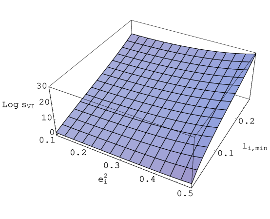
FIG. 1.: $\log{s_{\rm VI}}$ for the PEP as a function of $e^{2}_{i}$ and $\lambda_{i,min}$ for $y_{t}^{2}=0.5$, $\kappa=v$.

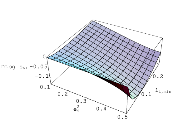
FIG. 2.: The difference between $\log{s_{\rm VI}}$ calculated from the PEP and $\log{s_{\rm VI}}$ calculated from the Landau gauge elementary field effective potential, as a function of $e^{2}_{i}$ and $\lambda_{i,min}$, for $y_{t}^{2}=0.5$, $\kappa=v$.

REFERENCES

- [1] M. Sher, Phys. Rep. 179 273 (1989).
- [2] M. Quiros, Constraints on the Higgs Boson Properties from the Effective Potential hep-ph/9703412 (to appear in Perspectives on Higgs Physics II Ed. G. L. Kane, World Scientific, Singapore.
- [3] M. Carena and C. E. M. Wagner, “Electroweak Baryogenesis and Higgs Physics”, (to appear in Perspectives on Higgs Physics II Ed. G. L. Kane, World Scientific, Singapore. hep-ph/9704347.
- [4] Will Loinaz and R. S. Willey, Gauge Dependence of Lower Bounds on the Higgs Mass Derived from Electroweak Vacuum Stability Constraints, hep-ph/9702321.
- [5] L. Dolan and R. Jackiw, Phys. Rev. D9 2904 (1974); L. Dolan and R. Jackiw, Phys. Rev. D9 3320 (1974); R. Jackiw, Phys. Rev. D9 1687 (1974).
- [6] K. Symanzik, Comm. Math. Phys. 16 48 (1970).
- [7] S. Coleman, Aspects of Symmetry, Cambridge Univ. Press (1985).
- [8] R. Rivers, “Path Integral Methods in Quantum Field Theory” (Cambridge Univ. Press, Cambridge 1987).
- [9] B. Basista and P. Suranyi, Phys. Rev. D48 3826 (1993).
-
[10]
N.K. Nielsen, Nucl. Phys. B101 173 (1975);
I.J.R. Aitchison & C.M. Fraser, Ann.Phys. 156 1 (1984);
J.R.S. do Nascimento & D. Bazeia, Phys. Rev. D35 2490 (1987). - [11] D. Metaxas and E. Weinberg, Phys. Rev. D53 836 (1996).
- [12] E. S. Fradkin and A. A. Tseytlin, Nucl. Phys. B234 509 (1984); A. O. Barvinski and G. A. Vilkovisky, Phys. Lett. B131 313 (1983); Phys. Rep. 119 1 (1985); G. A. Vilkovisky, in Quantum Theory of Gravity (Hilger, Bristol, 1984), p. 164; B. S. Dewitt, in Quantum Field Theory and Quantum Statistics (Hilger, Bristol, 1987), p. 191.
- [13] D. Boyanovsky, D. Brahm, R. Holman and D.-S. Lee, Phys. Rev. D54 1763 (1996).
- [14] P. A. M. Dirac, Lectures in Quantum Mechanics (Yeshiva University, New York, 1964). See also: A. Hansson, T. Regge and C. Teitelboim, Constrained Hamiltonian Systems (Academia Nazionale dei Lincei, Rome, 1976); M. Henneaux and C. Teitelboim, “Quantization of Gauge Systems”, Princeton University Press, 1992 and references therein. B. Hatfield: Quantum Field Theory of Point Particles and Fields, (Frontier in Physics, Addison Wesley, Redwood City, 1992).
- [15] R. Jackiw,Constrained Quantization Without Tears in Diverse Topics in Theoretical and Mathematical Physics, World Scientific, Singapore (1995).
- [16] L. Faddeev and A. Slavnov, Gauge Fields: an introduction to quantum theory. (Frontiers in Physics, Addison Wesley, Redwood City, 1991).
- [17] S. Coleman, E. Weinberg, Phys. Rev. D7 1888 (1973).
- [18] S. Elitzur, Phys. Rev. D12 3978 (1975).
- [19] G. S. Adkins, Phys. Rev. D27 1814 (1983).
- [20] K. Fujikawa, B.W. Lee, A.I. Sandia, Phys. Rev. D6 2923 (1972).
- [21] P.Q. Hung, Marc Sher, Phys. Lett. B374 138 (1996).
- [22] Masako Bando, Taichiro Kugo, Nobuhiro Maekawa, Hiroaki Nakano, Phys. Lett. B301 83 (1993).
- [23] Boris Kastening, Phys. Lett. B283 287 (1992).
- [24] J.A. Casas, J.R. Espinosa, M. Quiros, Phys. Lett. B342 171 (1995).
- [25] J.A. Casas, J.R. Espinosa, M. Quiros, Nucl. Phys. B436 3 (1995).
- [26] J.A. Casas, J.R. Espinosa, M. Quiros, Phys. Lett. B382 374 (1996).
- [27] I.S. Gradshteyn, I.W. Ryzhik, Table of Integrals, Series, and Products (Academic Press, New York, 1965).