Solutions to the Solar Neutrino Anomaly

Abstract

We present an updated analysis of astrophysical solutions, two-flavor MSW solutions, and vacuum oscillation solutions to the solar neutrino anomaly. The recent results of each of the five solar neutrino experiments are incorporated, including both the zenith angle (day-night) and spectral information from the Kamiokande experiment, and the preliminary Super-Kamiokande results. New theoretical developments include the use of the most recent Bahcall-Pinsonneault flux predictions (and uncertainties) and density and production profiles, the radiative corrections to the neutrino-electron scattering cross section, and new constraints on the Ga absorption cross section inferred from the gallium source experiments. From a model independent analysis, arbitrary astrophysical solutions are excluded at more that 98% C.L. even if one ignores any one of the three classes of experiment, relaxes the luminosity constraint, or allows more suppression of the ⁷Be than ⁸B flux. The data is well described by large and small mixing angle two-flavor MSW conversions, MSW conversions into a sterile neutrino with small mixing, or vacuum oscillations. We also present MSW fits for nonstandard solar models parameterized by an arbitrary solar core temperature or arbitrary ⁸B flux.

I Introduction

The solar neutrino problem currently provides one of the most compelling experimental signatures for the physics beyond the standard model. The Mikhyev-Smirnov-Wolfenstein (MSW) effect [1] via neutrino mass and mixing provides a complete explanation of the existing solar neutrino data, while astrophysical solutions, even those with drastic alterations of the standard solar model, simply fail. The difficulty with astrophysical explanations persists even if we ignore data of any one of the three kinds of experiments, i.e., the Homestake chlorine experiment [2], the water Čerenkov experiments of Kamiokande [3] and Super-Kamiokande [4], or the gallium experiments of SAGE [5] and GALLEX [6]. (The experimental results are summarized in Table I along with the SSM predictions [7].) The successful results of gallium source experiments [6, 5] and the excellent agreement between the standard solar model predictions and the recent helioseismology data further reinforce our confidence in neutrino oscillation solutions [8]. The new generation of solar neutrino experiments, such as Super-Kamiokande and Sudbury Neutrino Observatory (SNO), will provide critical tests of the MSW predictions for the neutrino energy spectrum distortion, the day-night rate asymmetry, and the charged-to-neutral current ratio.

In this paper we examine the current status of the solar neutrino problem for astrophysical solutions, MSW solutions, and vacuum oscillation solutions. The data as of February 1997, including the final Kamiokande results and the preliminary Super-Kamiokande data, are used. This is the first MSW analysis using the entire data of the Kamiokande spectrum and day-night asymmetry. We also incorporate the latest standard solar model with diffusion effects [7], the radiative corrections for the neutrino-electron scattering cross section [9], the improved determination of the ⁸B decay spectrum [10], and the constraint on the gallium cross section from the source experiments [11]. The calculations in this paper are described in detail in our previous works [12, 13, 14, 15, 16], including the model-independent analysis for astrophysical solutions, MSW calculations, the day-night effect, and consistent treatment of solar model uncertainties. We consider only two-flavor oscillations because of their simplicity and viability. We referred to Ref. [17] for a recent analysis for three-flavor oscillations and Ref. [18] for recent developments in neutrino physics.

This paper is organized as follows. In Section II we reexamine the general astrophysical solutions and show their failure with much stronger statistical significance than before. This is true even if we ignore any one of the three types of experiment or the solar luminosity constraint. We also discuss Monte Carlo evaluations of goodness of fit when the number of degrees of freedom (DOF) effectively becomes zero or negative. In Section III the constraints on the MSW parameters are updated. The Kamiokande spectrum result by itself excludes the adiabatic (horizontal) branch almost entirely. The MSW solutions with nonstandard core temperatures, and with nonstandard ⁸B flux, and oscillations to sterile neutrinos are also examined. Vacuum oscillation solutions are discussed in Section IV. We show that the Kamiokande spectrum data considerably restricts the allowed parameter space. The conclusions of our analysis are given in Section V.

II Astrophysical Solutions

The incompatibility of astrophysical solutions and the solar neutrino data has been investigated in many ways. These include the failure of explicit nonstandard solar models [19, 20], the comparison of the Homestake and Kamiokande results [21], lower core temperature fits [22, 12], and so on. One can generalize the argument against astrophysical solutions by a model independent analysis using $pp$, ⁷Be, ⁸B, and CNO fluxes as free parameters under minimal assumptions on the solar luminosity, the beta spectrum shape, and the detector cross sections. The details of our analysis is described in [13, 16] (similar analyses are found in [23, 24, 25, 26]). We will display the results of the fits in the $\phi({\rm Be})-\phi({\rm B})$ plane, both normalized to the SSM values ($\phi({\rm Be})_{\rm SSM}=5.15\times 10^{9}$ and $\phi({\rm B})_{\rm SSM}=6.62\times 10^{6}$ in units of cm^-2s^-1 [7]).

The constraints from individual data are shown in Fig. 1. The combined result from Kamiokande and Super-Kamiokande determines the ⁸B flux only. The CNO flux as well as the ⁷Be and ⁸B fluxes are used as free parameters in fitting the Homestake result. In fitting to the combined Ga result from SAGE and GALLEX, the $pp$ flux is also varied as a free parameter subject to the luminosity constraint.

A comparison of Fig. 1 with our original analysis in 1993 (Fig. 1 in Ref. [13]) displays a dramatic improvement in statistics, especially in the water Čerenkov data and the gallium data. The addition of the high-statistics Super-Kamiokande result with about 1000 events from the first 100 days has reduced the uncertainty in the ⁸B flux measurement in half. The low rate and the precision of the gallium result alone impose serious problems for astrophysical solutions. The ⁸B flux allowed by the Homestake and gallium data each is smaller than the Kamiokande–Super-Kamiokande measurement for almost the entire range of the ⁷Be flux. In addition the Homestake and gallium together are incompatible, since for $\phi({\rm Be})\sim 0$ and $\phi({\rm B})\sim 0$, the gallium data requires the CNO flux to be $\sim 0$, while the Homestake data requires the CNO flux 4.9 times larger than the SSM value.

The severity of the problem with astrophysical solutions can be seen by applying the joint analysis to all the data, shown in Fig. 2. We allow the ⁷Be flux to be negative. The best fit of the combined observations is in the non-physical region: $\phi({\rm Be})/\phi({\rm Be})_{\rm SSM}=-0.6\pm 0.4$ and $\phi({\rm B})/\phi({\rm B})_{\rm SSM}=0.4\pm 0.05$ with $\chi^{2}_{\rm min}=0.5$ for 3 data points, one luminosity constraint, and four free parameters: i.e., zero degrees of freedom (DOF). Within physical parameter space ($\phi({\rm Be})\geq 0$ and $\phi({\rm B})\geq 0$), the best fit is $\phi({\rm Be})/\phi({\rm Be})_{\rm SSM}<0.1$ and $\phi({\rm B})/\phi({\rm B})_{\rm SSM}=0.38\pm 0.05$ with $\chi^{2}_{\rm min}=9.2$. The usual prescription for goodness of fit (GOF) evaluations [28] does not apply since we have zero DOF. (Later we will encounter fits with negative DOF). In addition the probability distribution is non-Gaussian due to the physical constraints, i.e., the fluxes should be non-negative. Generalization of GOF by employing the Monte Carlo method is necessary.

GOF in this case is defined by the probability to obtain $\chi^{2}_{\rm min}$ as large as 9.2 or larger by chance due to the experimental uncertainties, if the best fit fluxes are true. Our Monte Carlo construction is (1) to take the central flux values of the fit, (2) calculate the solar neutrino rates for the three experiments, (3) generate Monte Carlo distributions for each experiment assuming the actual experimental uncertainties (7.7, 7.4, and 9.7% for the Homestake, Kamiokande/Super-Kamiokande, and gallium experiments, respectively), (4) for each Monte Carlo data set, apply our model independent analysis to obtain the $\chi^{2}$ minimum. Note that when one has $N$ parameters and $M$ constraints with Gaussian errors and $N>M$, this procedure can be done analytically, reproducing the usual $\chi^{2}$ distribution for $N-M$ dimensions [29].

The Monte Carlo distribution of the $\chi^{2}$ minima is shown in Fig. 3; the $\chi^{2}_{\rm min}=9.2$ from the actual data is also indicated. The probability of getting $\chi^{2}$ minimum larger than 9.2 by chance is 0.6%. That is, our model independent analysis excludes the best fit astrophysical solution at the 99.4% C.L.

Next we consider the same analysis but ignoring one of the constraints. Fig. 4, 5, and 6 show the results each without the Homestake data, the water Čerenkov data, and the gallium data, respectively. Fig. 7 is the result with all experiments, but without the luminosity constraint. (Violations of the luminosity constraint would be possible if the properties of the solar core were somehow varying on a time scale short compared with $10^{4}$ years.) The corresponding GOF of the best fit in the physical region is 98.9, 98.3, 98.9, and 98.3% C.L., respectively. Although the constraints on the fluxes are somewhat relaxed by ignoring one of the data or the luminosity constraint, the essential problem with the poor fit remains. In addition one can also see the persistent problem of the strong suppression of the ⁷Be flux, which is difficult to obtain by astrophysical effects in general.

III MSW Solutions

A Kamiokande spectrum and day-night data

The Kamiokande experiment has completed its measurements and published the results of total rate, spectrum data, and day-night data [3]. The MSW parameters can be constrained by those results. Note that the spectrum distortions and day-night time-dependence are not expected with standard neutrino physics and are powerful indicators of physics beyond the standard model. The spectrum shape measured in Kamiokande is consistent with the one expected from the undistorted ⁸B $\beta$-decay spectrum albeit the uncertainties are large. The shape is inconsistent with the strong suppressions at large energies expected in the MSW adiabatic branch ($\Delta m^{2}\sim 10^{-4}$ eV² and $\sin^{2}2\theta\sim 10^{-4}-0.1$), and the data exclude the region almost entirely as shown in Fig. 8. This exclusion is simply due to lack of distortions in the data and independent of the uncertainties in the initial ⁸B flux. The data, however, do not constrain the nonadiabatic (diagonal) branch, in which spectrum distortions are smaller.

The day-night result was published as one day-time rate and five bins for night-time bins. The binning was $\cos\theta=0-0.2$, $0.2-0.4$, … $0.8-1$, where $\theta$ is the angle between the direction to the Sun and the nadir at the detector. Within the experimental uncertainties the six bins are consistent and thus exclude a large region in which day-night asymmetries due to the Earth effect are expected. The excluded region is shown in Fig. 8.

The allowed parameter space from the total Kamiokande rate is shown in Fig. 9. This constraint is model dependent and we have assumed the Bahcall-Pinsonneault model (1995) [7] including its uncertainties. In this and other fits the correlation in the theoretical uncertainties between the flux components and between the experiments are included.

Unfortunately we cannot combine the spectrum and day-night data since the errors in those are strongly correlated and the correlation matrix is unpublished. Fig. 10 and 11 show the allowed region when the total rate is combined with the spectrum data and day-night data, respectively.

B Preliminary results from Super-Kamiokande

Recently the Super-Kamiokande collaboration reported the results of about 1000 events from the first 100 days of data [4]. The total rate (see Table I) is consistent with the previous Kamiokande rate, and new uncertainties are much smaller. When combined with the Kamiokande total rate, the error is reduced almost by half. The new constraint is shown in Fig. 12. The uncertainties in the MSW parameter space are now dominated by the ⁸B flux error in the solar model calculations ($\sim$ 15%). Future measurements of model-independent quantities such as the spectrum shape and day-night effect and also the charged-to-neutral current ratio in SNO, are essential to confirm the MSW interpretation and to improve the determination of the MSW parameters.

C MSW combined results

We next consider the MSW constraint including the Homestake and gallium data. The two separate allowed regions are shown in Fig. 13. The fit includes Kamiokande day-night data and the averaged Super-Kamiokande data. (The allowed regions are essentially identical even if the Kamiokande spectrum data are used.) Both allowed regions provide a good fit. The $\chi^{2}$ minimum for 7 degrees of freedom is 5.9 (55% C.L.) and 6.4 (49% C.L.) for the small-angle and large-angle solution, respectively. (Details are listed in Table II.) The fit for the large-angle solution improved from previous analyses (see for example Ref [15]) due to the larger ⁸B flux in the new SSM and a new, smaller Kamiokande and Super-Kamiokande rate, both of which reduces the relative difference between the Homestake rate and the Kamiokande/Super-Kamiokande rate and allows energy-independent flux reduction as expected in the large-angle region.

We have also considered oscillations to sterile neutrinos [30]. The GOF for the large angle region is 94% C.L. However, the 95% allowed region defined by $\chi^{2}<\chi^{2}_{\rm min}+6.0$ does not appear in the $\sin^{2}2\theta$ – $\Delta m^{2}$ parameter space (Fig. 14 and Table III). The large angle solution for sterile neutrinos is also severely constrained by big bang nucleosynthesis [30, 31].

While nonstandard solar models, as discussed in Section II, cannot solve the solar neutrino problem, the MSW effect can be also considered with nonstandard solar models [12, 15]. Many of those models may be parameterize by nonstandard core temperature ($T_{C}$) or simply a nonstandard ⁸B flux, whose uncertainties might be larger than the SSM estimate. We consider joint fits of $T_{C}$ or ⁸B flux, in addition to the MSW parameters.

When $T_{C}$ is used as a free parameter, the neutrino fluxes can be scaled according to the power law. From the Monte Carlo investigation of the SSM, the indices of the power law are obtained in Ref. [32], based on the Monte Carlo SSMs by Bahcall and Ulrich [19]. The combined Homestake, gallium, Kamiokande, and Super-Kamiokande data constrain

$$T_{C}/T_{C}^{\rm SSM}=0.99^{+0.02}_{-0.03}\hskip 10.00002pt(1\sigma),$$ (1)

and $T_{C}/T_{C}^{\rm SSM}=0.95-1.02$ for 95% C.L., where $T_{C}^{\rm SSM}$ is the the SSM value ($1.567\times 10^{7}$K). This result is in excellent agreement with the SSM range $1\pm 0.006$ [19]: the data are consistent with the SSM prediction in the presence of the MSW effect. Our likelihood for $T_{C}$ is shown in Fig. 15. The corresponding MSW parameter space is shown in Fig. 16.

Next the ⁸B flux is used as a free parameter, the combined data determines

$$\phi({\rm B})/\phi({\rm B})_{\rm SSM}=0.76^{+0.38}_{-0.30}\hskip 10.00002pt(1\sigma).$$ (2)

and 0.31 – 1.50 for 95% C.L. Although the uncertainty is large, the result is consistent with the SSM range $1^{+0.14}_{-0.17}$ [7]. Our likelihood for $\phi({\rm B})$ and the corresponding MSW regions are shown in Fig. 17 and 18.

IV Vacuum Oscillation Solutions

The simple two-flavor vacuum oscillations are still a phenomenologically viable solution [33]. Those solutions require tuning of $\Delta m^{2}$ and the Sun-Earth distance at the 5% level to explain the observations, which is a conceptual setback.

Some parameter space for the vacuum oscillation for $\Delta m^{2}\sim 10^{-10}$ eV² predicts a relatively strong energy dependence, and the recent Kamiokande spectrum data alone can exclude a wide range of parameters, as shown in Fig. 19. When combined with the results of Homestake, gallium, and Super-Kamiokande, we find three separate allowed regions within a narrow range of parameters [$\Delta m^{2}=(5-8)\times 10^{-11}$ eV² and $\sin^{2}2\theta=0.65-1$] as shown in Fig. 20. The GOF for the best fit parameters is 9.9 for 9 DOF, which is acceptable. Details of the fits are listed in Table IV For comparison we show five allowed regions when the Kamiokande spectrum data are ignored Fig. 21).

V Conclusions

Although the general scope of the solar neutrino problem has not chanced since the first result of the gallium experiment in 1992, the improved accuracy of the solar neutrino data provide a more robust assessment of solutions. The astrophysical solutions in general have difficulties unless all experiments are wrong, or at least two out of three data and the SSM are wrong.

The MSW effect provides viable solutions: the small mixing-angle solution ($\sin^{2}2\theta\sim 0.008$ and $5\times 10^{-6}$ eV²) and the large-angle solution ($\sin^{2}2\theta\sim 0.6$ and $1.6\times 10^{-5}$ eV²), assuming the latest SSM by Bahcall and Pinsonneault. Oscillations to sterile neutrinos are possible, but only for small angles. When the core temperature or the ⁸B flux is used as a free parameter, the joint data determines those at the 3% and 30% level, respectively. Those ranges are consistent with the SSM predictions. Vacuum oscillations are still viable for $\Delta m^{2}\sim 6\times 10^{-11}$ eV² and $\sin^{2}2\theta\sim 0.9$.

The Kamiokande day-night data and spectrum data each exclude a large parameter space for MSW, independent of SSM predictions. We expect Super-Kamiokande will provide those with much improved accuracy and eventually, along with the SNO neutral current measurement, single out the solution of the solar neutrino problem.

TABLE I.: The standard solar model predictions of Bahcall and Pinsonneault (BP SSM) [7] and the results of the solar neutrino experiments.

	BP SSM	Experiments
Homestake	9.3 ${}^{+1.2}_{-1.4}$ SNU	2.55 $\pm$ 0.14 $\pm$ 0.14 SNU (0.273 $\pm$ 0.021 BP SSM)
Kamiokande		2.80 $\pm$ 0.19 $\pm$ 0.33 a (0.423 $\pm$ 0.058 BP SSM)
Super-Kamiokande	6.62 ${}^{+0.93}_{-1.12}$ a	2.51 ${}^{+0.14}_{-0.13}$ $\pm$ 0.18 a ($0.379\pm 0.034$ BP SSM)
Combined		2.586 $\pm$ 0.195 a (0.391 $\pm$ 0.029 BP SSM)
SAGE		69 $\pm$ 10 ${}^{+5}_{-7}$ SNU (0.504 $\pm$ 0.089 BP SSM)
GALLEX	137 ${}^{+8}_{-7}$ SNU	69.7 $\pm$ 6.7 ${}^{+3.9}_{-4.5}$ SNU (0.509 $\pm$ 0.059 BP SSM)
Combined		69.5 $\pm$ 6.7 SNU (0.507 $\pm$ 0.049 BP SSM)

TABLE II.: The best fit parameters, the $\chi^{2}$ minimum, and confidence levels of GOF for the combined MSW fits.

	Small Angle	Large Angle
$\sin^{2}2\theta$	$8.2\times 10^{-3}$	0.63
$\Delta m^{2}$ (eV2)	$5.1\times 10^{-6}$	$1.6\times 10^{-5}$
$\chi^{2}$ (7 d.f.)	5.9	6.3
$P$ (%)	45	49

TABLE III.: The best fit parameters, $\chi^{2}$ minimum, and GOF for the combined MSW fits for oscillations to sterile neutrinos.

	Small Angle	Large Angle
$\sin^{2}2\theta$	$1.0\times 10^{-2}$	0.72
$\Delta m^{2}$ (eV2)	$4.0\times 10^{-6}$	$8.9\times 10^{-6}$
$\chi^{2}$ (7 d.f.)	6.7	13.7
$P$ (%)	54	94

TABLE IV.: The best fit parameters, $\chi^{2}$ minimum, and GOF for the combined vacuum oscillation fits including the Kamiokande spectrum data.

	Solution 1	Solution 2	Solution 3
$\sin^{2}2\theta$	0.83	0.90	1.0
$\Delta m^{2}$ (eV2)	$7.9\times 10^{-11}$	$6.6\times 10^{-11}$	$5.2\times 10^{-11}$
$\chi^{2}$ (9 d.f.)	11.4	9.9	11.9
$P$ (%)	75	64	78

FIG. 1.: The constraints on the ⁷Be and ⁸B fluxes at 90% C.L. from the Homestake result (below the dotted line), the combined Kamiokande and Super-Kamiokande results (between the dot-dashed lines), and the combined SAGE and GALLEX results (below the dashed line). The SSM range is also shown (solid line, 90% C.L.)

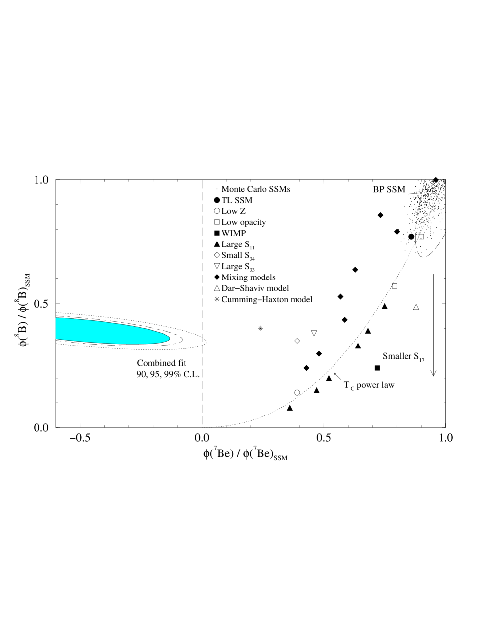
FIG. 2.: The constraints from the combined Cl, Ga, and Čerenkov experiments at 90, 95, and 99% C.L.  Also shown are the Bahcall-Pinsonneault SSM region at 90% C.L. [7], the core temperature power law and standard and nonstandard solar models including the recent ³He diffusion model by Cunning and Haxton [34] (see Ref. [16] for references for the other models). A smaller $S_{17}$ cross section moves the solar model predictions to a smaller ⁸B flux as indicted by the arrow.

FIG. 3.: The Monte-Carlo distribution of $\chi^{2}$ minima when the best fit fluxes in the physical region ($\phi({\rm Be})/\phi({\rm Be})_{\rm SSM}=0$ and $\phi({\rm B})/\phi({\rm B})_{\rm SSM}=0.35$) are assumed. The actual $\chi^{2}$ minimum of the combined observations are indicated by the arrow. The best fit astrophysical solution is excluded at the 99.4% C.L.

FIG. 4.: The result with the water Čerenkov and gallium data only.

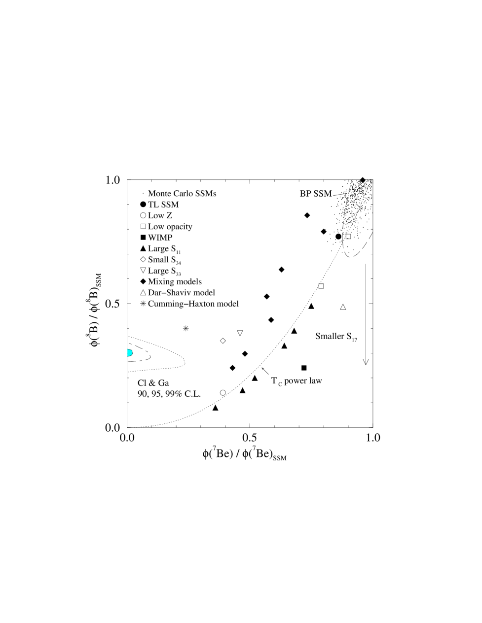
FIG. 5.: The result with the Homestake and gallium data only.

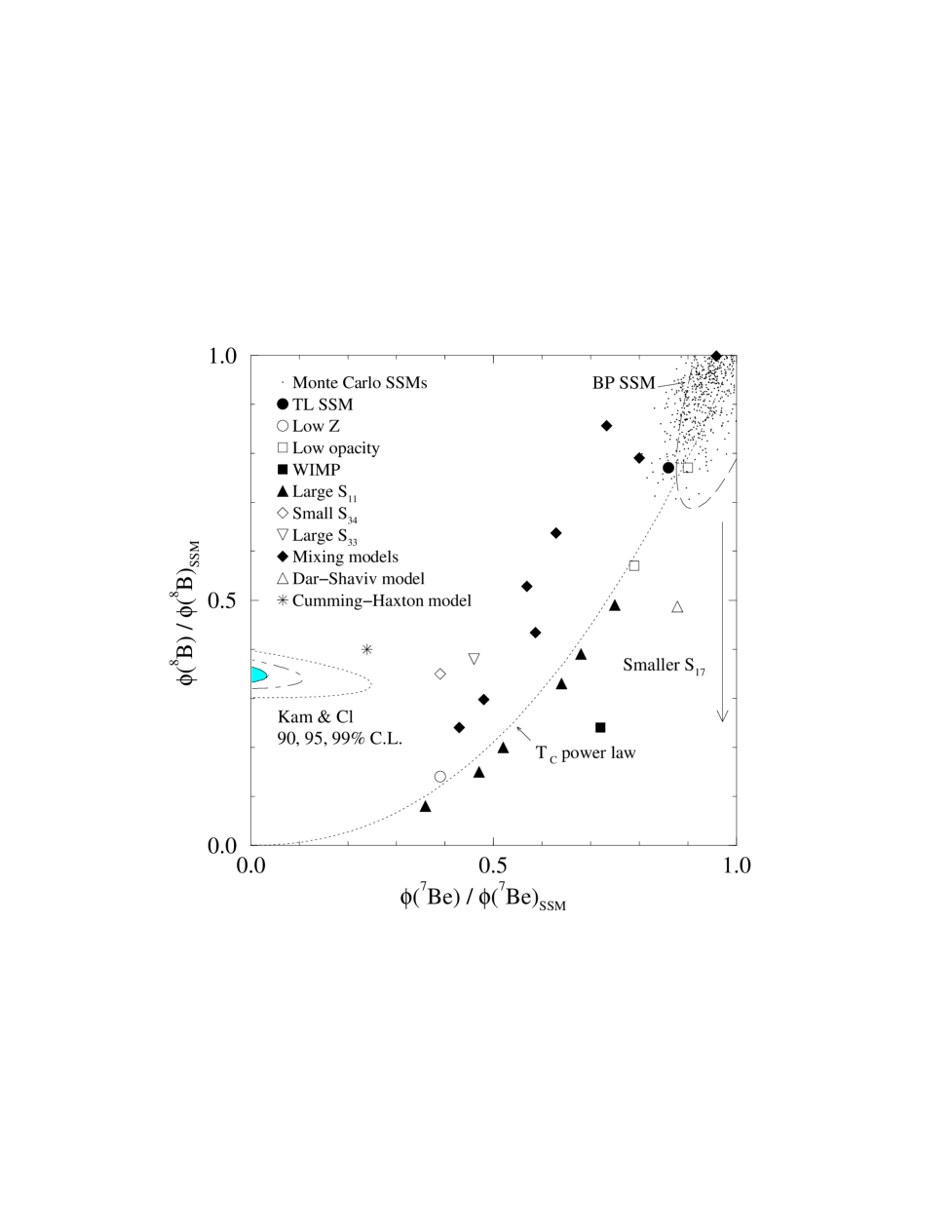
FIG. 6.: The result with the Homestake and water Čerenkov data only.

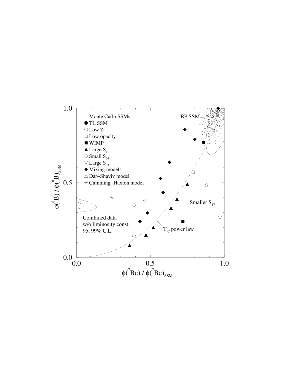
FIG. 7.: The result with the combined data but without imposing the luminosity

constraint.

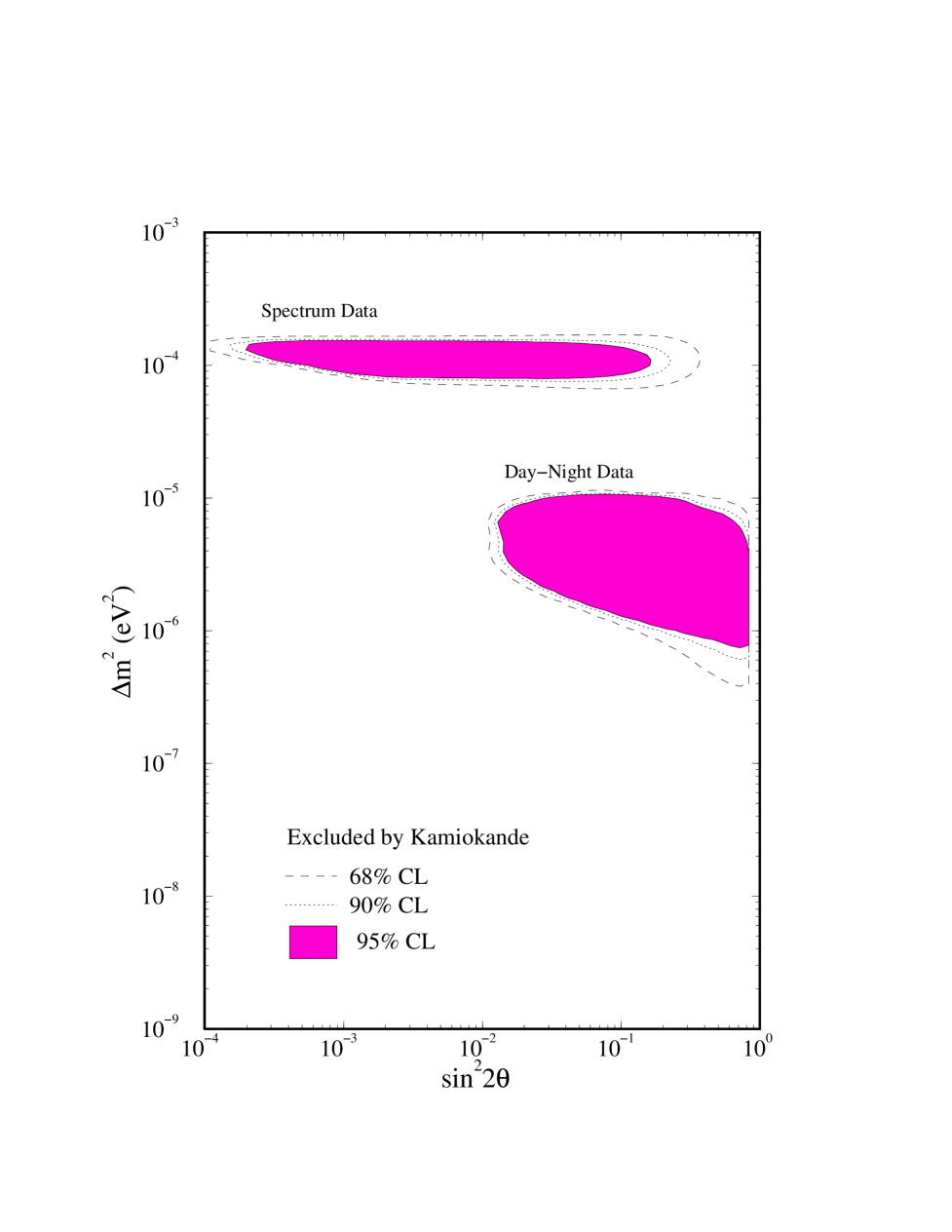
FIG. 8.: The MSW parameter space excluded by the Kamiokande spectrum data and day-night data.

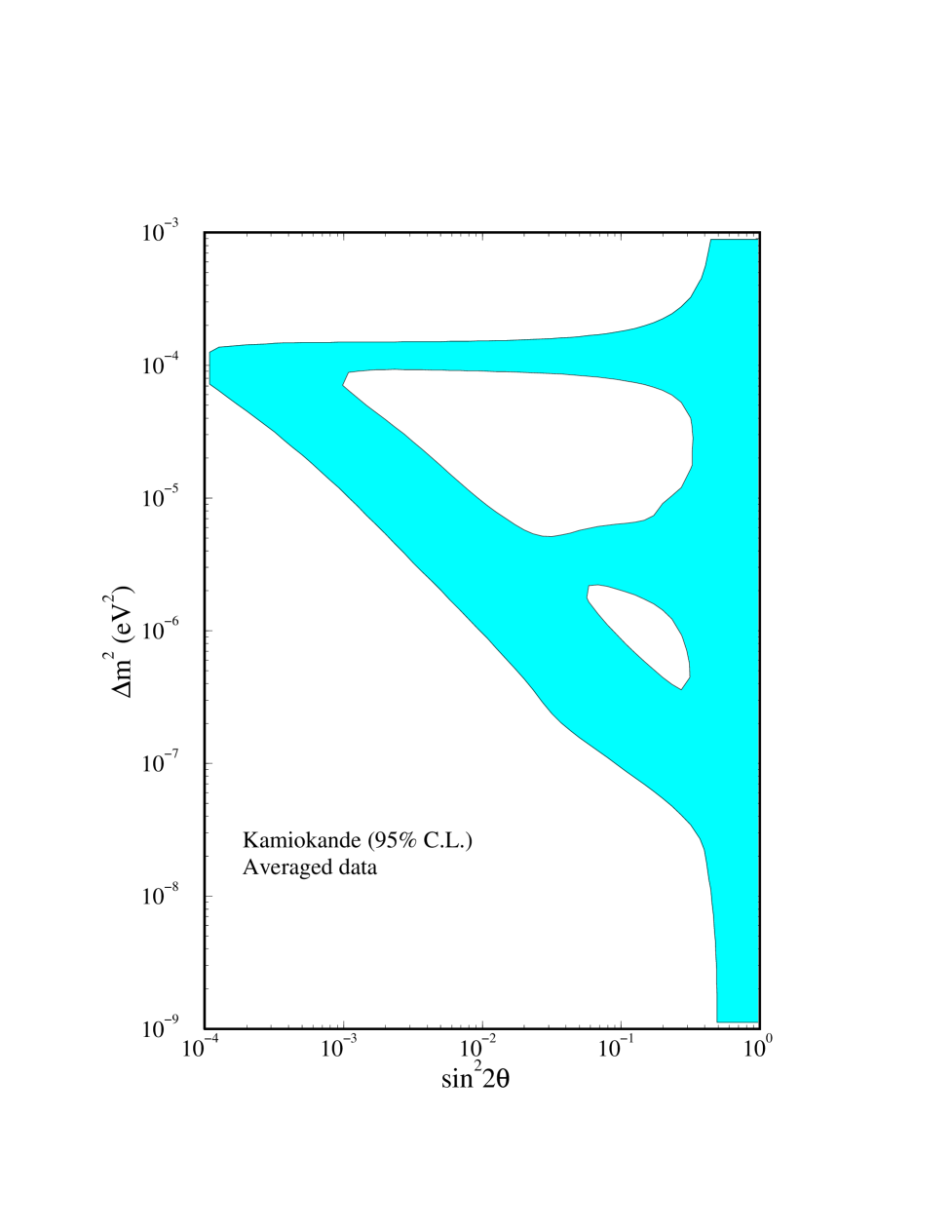
FIG. 9.: The MSW parameter space allowed by the Kamiokande total rate.

FIG. 10.: The MSW parameter space allowed by the Kamiokande total rate and spectrum data.

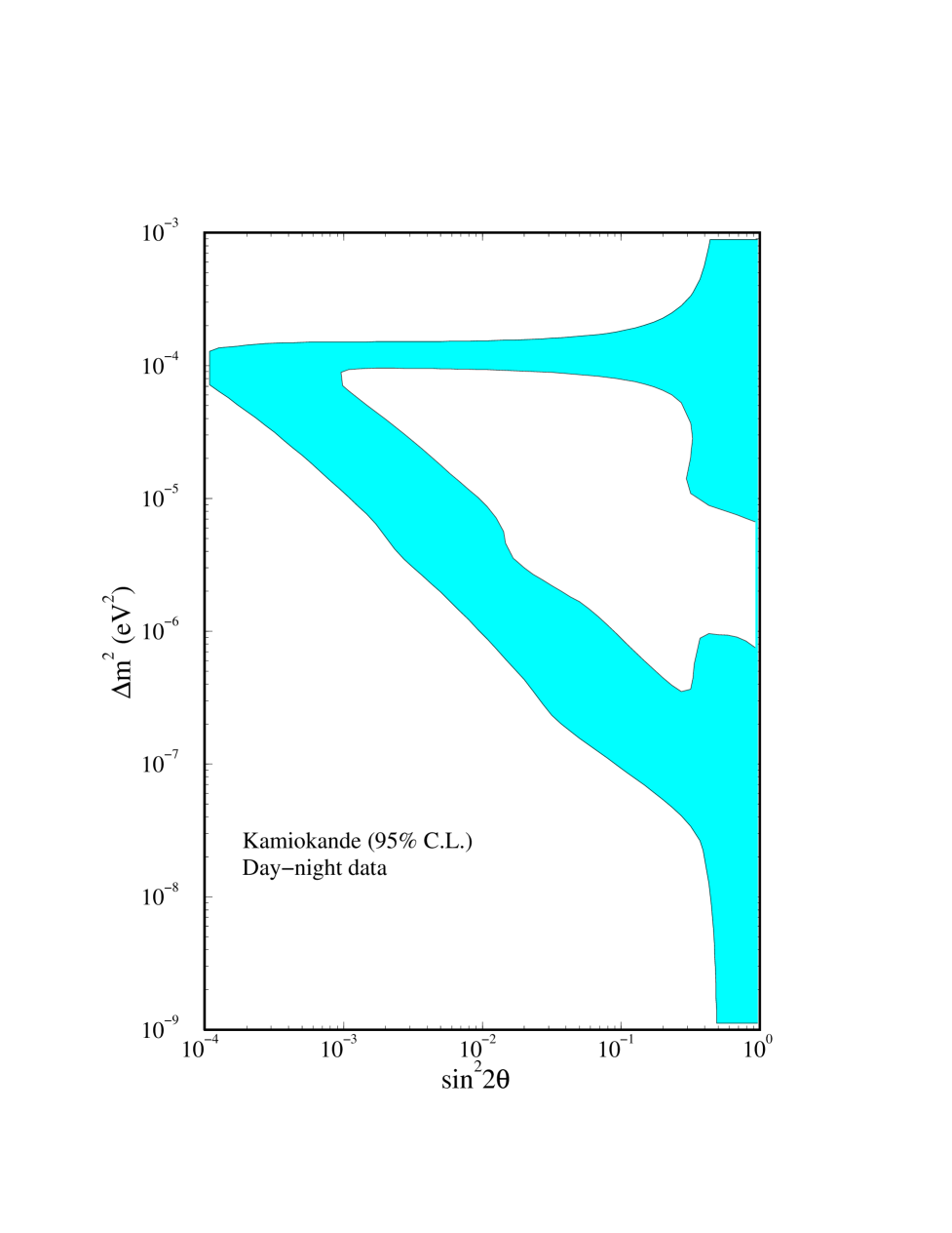
FIG. 11.: The MSW parameter space allowed by the Kamiokande total rate and day-night data.

FIG. 12.: The comparison of the MSW parameter space allowed by the Kamiokande total rate (shaded region) and the combined Kamiokande and preliminary Super-Kamiokande rate (dashed lines). The theory error ($\sim$ 15%) is the leading uncertainty in the combined fits.

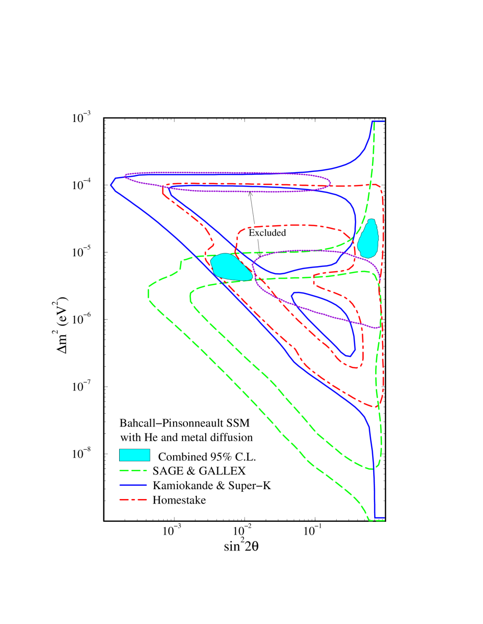
FIG. 13.: The result of the MSW parameter space (shaded regions) allowed by the combined observations at 95% C.L. assuming the Bahcall-Pinsonneault SSM with He diffusion. The constraints from Homestake, combined Kamiokande and Super-Kamiokande, and combined SAGE and GALLEX are shown by the dot-dashed, solid, and dashed lines, respectively. Also shown are the regions excluded by the Kamiokande spectrum and day-night data (dotted lines).

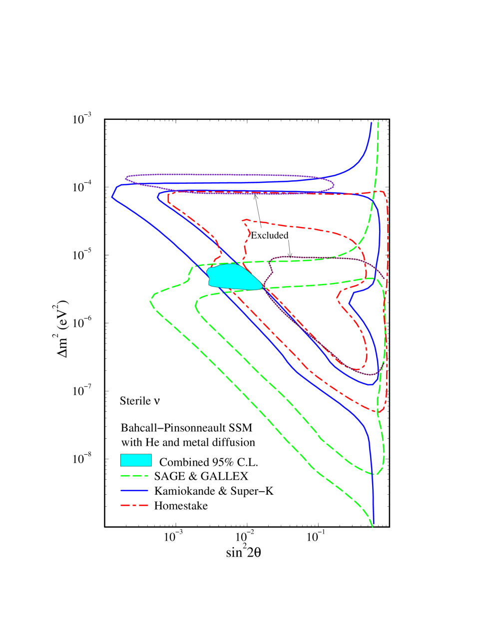
FIG. 14.: Same as Fig. 13 except that this is for oscillations to sterile neutrinos.

FIG. 15.: The likelihood distribution of the core temperature from the simultaneous MSW fit to the combined observations.

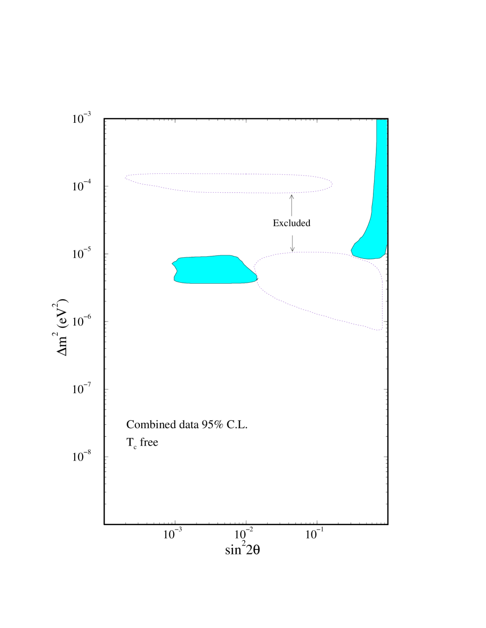
FIG. 16.: The MSW parameter space allowed by the combined observations when the core temperature is used as a free parameter. The model independent exclusion regions by the Kamiokande spectrum and day-night data are also shown.

FIG. 17.: The likelihood distribution of the core temperature from the simultaneous MSW fit to the combined observations.

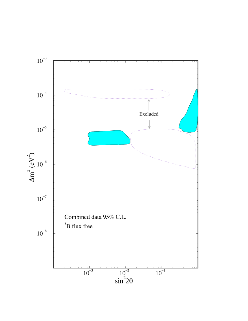
FIG. 18.: The MSW parameter space allowed by the combined observations when the ⁸B flux is used as a free parameter. The model independent exclusion regions by the Kamiokande spectrum and day-night data are also shown.

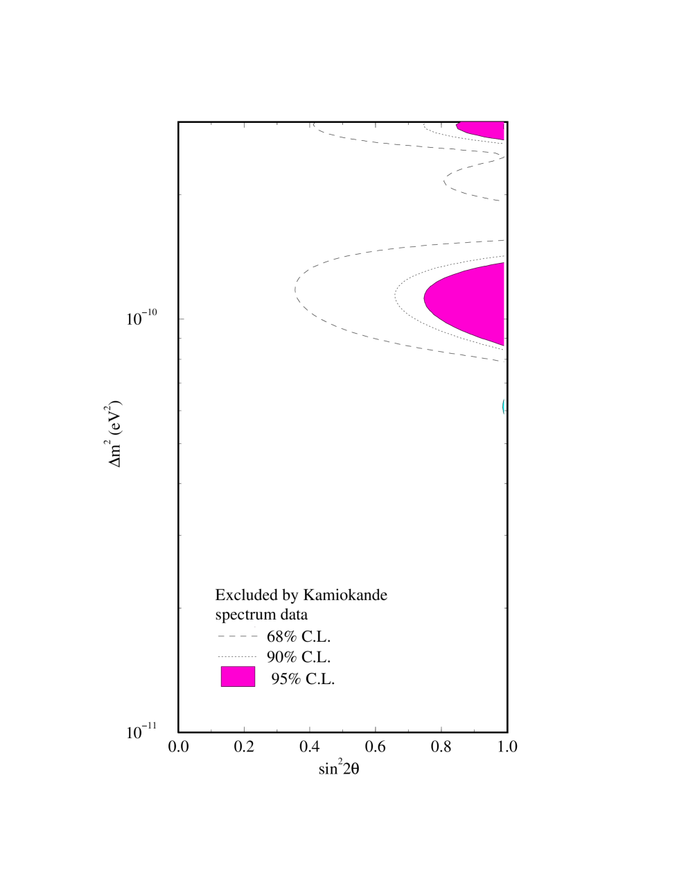
FIG. 19.: The vacuum oscillation parameter space excluded by the Kamiokande spectrum data.

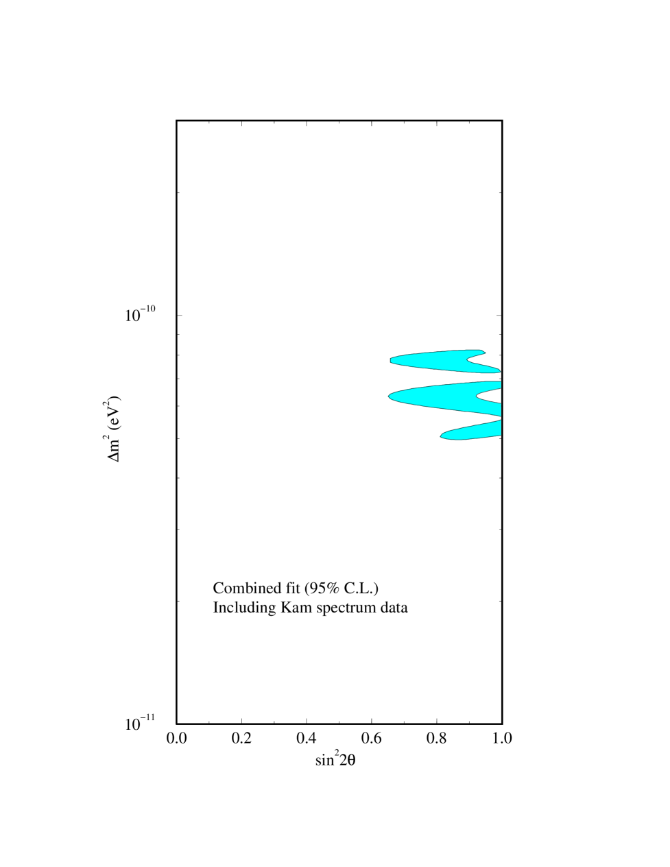
FIG. 20.: The vacuum oscillation parameter space allowed by the combined observations including the Kamiokande spectrum data.

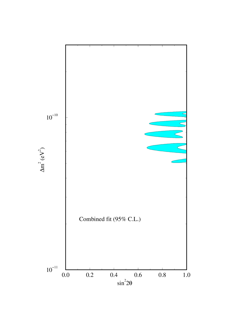
FIG. 21.: The vacuum oscillation parameter space allowed by the combined observations but without the Kamiokande spectrum data.