UCD-97-13
May, 1997

DETECTING AND STUDYING HIGGS BOSONS 

We review the ability of the LHC (large hadron collider), NLC (next linear lepton collider) and FMC (first muon collider) to detect and study Higgs bosons, with emphasis on the Higgs bosons of extended Higgs sectors, especially those of the minimal supersymmetric standard model (MSSM). Particular attention is given to means for distinguishing the lightest neutral CP-even Higgs boson of the MSSM from the single Higgs boson of the minimal Standard Model (SM).

1 Introduction

Indirect evidence from precision electroweak analyses is increasingly suggestive that there is a relatively light Higgs boson with SM-like properties. $\!{}^{{\bf?}}$ Since there is also a complete absence to date of any signals for new physics, the SM with a single neutral Higgs boson ($h_{\rm SM}$) remains a very viable model. However, there are simple extensions of the one-Higgs-doublet  SM Higgs sector that are equally consistent with all known theoretical and phenomenological constraints. $\!{}^{{\bf?}}$ Models containing extra Higgs doublets and/or singlets are the most attractive. Such models automatically preserve the custodial SU(2) symmetry tree-level prediction of $\rho\equiv m_{W}^{2}/[m_{Z}^{2}\cos^{2}\theta_{W}]=1$.

• In a general two-Higgs-doublet model (2HDM), there are three neutral CP-mixed Higgs eigenstates ($h_{1,2,3}$) and a charged Higgs pair ($H^{\pm}$). In the CP-conserving limit, the neutral sector of the 2HDM divides into two CP-even states ($h^{0}$ and $H^{0}$) and one CP-odd state ($A^{0}$). The Higgs sector of the MSSM is a highly constrained CP-conserving 2HDM.

• If a single complex Higgs singlet field is added to the 2HDM, then there will be a pair of charged Higgs bosons and, in the CP-conserving limit, three CP-even and two CP-odd neutral states. In the CP-violating case, there would simply be five CP-mixed neutral states. The Higgs sector of the next-to-minimal supersymmetric model (NMSSM) is a constrained two-doublet, one-singlet model that is often taken to be CP-conserving, but could also be explicitly or spontaneously CP-violating.

Models containing triplet Higgs fields (in addition to at least one doublet, as required to give masses to quarks and leptons) are also frequently discussed. $\!{}^{{\bf?}}$ However, lack of space precludes discussing such models here. A brief review of some recent phenomenology is given in the Snowmass96 Higgs boson summary report $\!{}^{{\bf?}}$ (hereafter referred to as Higgs96).

In most extended Higgs sector models, it is very natural to be in a decoupling regime in which the lightest Higgs boson ($h^{0}$) is neutral and CP-even and has very SM-like properties. Other Higgs bosons would be heavier; depending on the model, the additional neutral scalars could be of pure or mixed CP nature.

Supersymmetric models provide a particularly natural framework for light scalars, and are attractive in many ways, including the fact that they resolve the naturalness and hierarchy problems associated with the SM Higgs sector. The minimal Higgs sector required in order to give both up and down quarks masses and to avoid anomalies consists of two doublets. Two doublets also imply quite accurate gauge coupling unification if the supersymmetric partners of the SM particles have masses below 1 to 10 TeV. More doublets would destroy this unification. In the CP-conserving MSSM 2HDM Higgs sector with physical eigenstates $h^{0},H^{0},A^{0},H^{\pm}$, the Higgs boson masses and couplings are entirely specified by just two parameters at tree-level. These are normally taken to be $m_{A^{0}}$ and $\tan\beta$ (the ratio of vacuum expectations values for the neutral members of the two doublets). When $m_{A^{0}}\gg m_{Z}$ (as is natural in a GUT context), the $h^{0}$ remains light ($m_{h^{0}}\mathrel{\raise 1.29167pt\hbox{$<$\kern-7.5pt\lower 4.30554pt\hbox{$\sim$}}}130\,{\rm GeV}$ $\!{}^{{\bf?},{\bf?}}$) and is very SM-like while the other scalars have $m_{H^{0}}\sim m_{H^{\pm}}\sim m_{A^{0}}$ and decouple from $ZZ,WW$.

However, there is no guarantee that the supersymmetric model Higgs sector will consist of just two doublets. In the next-to-minimal supersymmetric extension of the SM (NMSSM), $\!{}^{{\bf?},{\bf?}}$ a complex singlet superfield ($\widehat{N}$) is added to the two doublet superfields ($\widehat{H}_{1}$ and $\widehat{H}_{2}$) of the MSSM. The scalar component of the singlet superfield joins with the scalar components of the two doublet superfields to form a two-doublet, one-singlet Higgs sector. One or more such singlet superfields are a common feature of the low energy supersymmetric effective field theories that emerge from the typical super string compactification. Singlets leave intact the compelling attractive theoretical successes of the MSSM. In particular, gauge coupling unification is unmodified. The NMSSM has the added virtue of allowing for a natural source for a $\sim\,{\rm TeV}$-scale $\mu$ parameter through a $\widehat{H}_{1}\widehat{H}_{2}\widehat{N}$ term in the superpotential when the scalar component of $\widehat{N}$ acquires a non-zero vacuum expectation value. However, adding one or more singlet fields could have a substantial impact on the ease with which the Higgs bosons of the model can be discovered and studied. In the GUT context, a decoupling limit in which one of the CP-even Higgs bosons remains light ($m_{h^{0}}\mathrel{\raise 1.29167pt\hbox{$<$\kern-7.5pt\lower 4.30554pt\hbox{$\sim$}}}150\,{\rm GeV}$ assuming that the coupling $\lambda$ characterizing the strength of the cubic singlet superfield term, $\lambda\widehat{N}^{3}$, in the superpotential remains perturbative during evolution to the GUT scale) and has SM-like couplings, the other Higgs bosons being heavy, remains a possibility. The $h^{0}$ would then be easily discovered, while the discovery of the heavier Higgs bosons would not be guaranteed. But, it is also very possible that there will be two or even three relatively light CP-even Higgs scalars that share the $ZZ,WW$ coupling strength. In this case, the strength of the signals for any one of these scalars is reduced relative to a SM Higgs boson of the same mass. An important question is whether discovery of at least one of the Higgs bosons of the model can then be guaranteed at future, if not present, accelerators.

Given the possibility (or in the MSSM, the probability) that the extended Higgs sector will have a light SM-like $h^{0}$, it is clear that discriminating between it and the minimal SM Higgs sector will require either the detection of differences between the $h^{0}$ properties and those predicted for the $h_{\rm SM}$ (at a precision level) or direct observation of the heavier scalar eigenstates. It is the prospects for success in these two tasks upon which much of this review focuses. Both tasks become increasingly difficult as the mass scale of the heavier Higgs boson eigenstates increases.

The outline of the rest of this review is the following. In Section 2, we explore the precisions expected for measurements of the properties of a SM-like Higgs boson at various accelerators. Our primary focus will be on the next generation of machines: the Large Hadron Collider (LHC), a next linear $e^{+}e^{-}$ collider (NLC), and a possible future $\mu^{+}\mu^{-}$ collider (FMC). Expectations for LEP2 and Tev33 will also be noted. In Section 3, we examine search strategies for and the measurement of the properties of Higgs bosons with very non-SM-like properties, in particular the heavier Higgs bosons of the MSSM. Section 4 presents conclusions. This review is designed to give an overview of the current expectations and strategies, and consequently does not include many details. Familiarity with the basics presented in the Higgs Hunters Guide $\!{}^{{\bf?}}$ is presumed. The review is designed to be read as a guide to the recent DPF95 $\!{}^{{\bf?}}$ and Higgs96 $\!{}^{{\bf?}}$ reviews, the NLC Physics report, $\!{}^{{\bf?}}$ and the muon-collider $s$-channel Higgs physics study. $\!{}^{{\bf?}}$ The LEP2 $\!{}^{{\bf?}}$ and European $e^{+}e^{-}$ collider $\!{}^{{\bf?}}$ study group reports are also valuable references.

2 Discovery and Precision Measurements of a SM-like Higgs

There is no question that a SM-like Higgs boson with mass below 1 TeV or so can be discovered at the LHC assuming that the latter reaches its design goal of $L=100~{}{\rm fb}^{-1}$ per year per detector. Indeed, for much of the mass range in which the Higgs sector is weakly-coupled ($m_{h_{\rm SM}}\mathrel{\raise 1.29167pt\hbox{$<$\kern-7.5pt\lower 4.30554pt\hbox{$\sim$}}}600\,{\rm GeV}$) significantly less integrated luminosity is required. The discovery reach of the NLC  will be entirely determined by the available energy, $\sqrt{s}$. A $\sqrt{s}=500\,{\rm GeV}$ NLC would discover a SM-like Higgs boson with $m_{h_{\rm SM}}\leq 350\,{\rm GeV}$, assuming $L=50~{}{\rm fb}^{-1}$ is accumulated. Much less luminosity is required for masses in the range $\mathrel{\raise 1.29167pt\hbox{$<$\kern-7.5pt\lower 4.30554pt\hbox{$\sim$}}}150\,{\rm GeV}$ predicted for the SM-like supersymmetric model Higgs boson in the MSSM or NMSSM. (Summary figures can be found in DPF95. $\!{}^{{\bf?}}$) Finally, a FMC run at $\sqrt{s}\simeq m_{h_{\rm SM}}$ would produce a SM-like Higgs boson at a very high rate, provided $m_{h_{\rm SM}}<2m_{W}$. The real issue is the precision with which the properties of the SM-like Higgs boson can be measured at the three machines. The most extensive exploration of this matter appears in the Higgs96 review. $\!{}^{{\bf?}}$ There, errors are estimated assuming that multi-year running will achieve the following accumulated luminosities at the different accelerator facilities: $L=300~{}{\rm fb}^{-1}$ for both ATLAS and CMS at the LHC; $L=200~{}{\rm fb}^{-1}$ in $\sqrt{s}=500\,{\rm GeV}$ operation at the NLC; $L=50~{}{\rm fb}^{-1}$ for $\gamma\gamma$ collisions at the NLC operating in the photon-collider mode with $E_{e^{+}e^{-}}\sim m_{h_{\rm SM}}/0.8$; and $L=200~{}{\rm fb}^{-1}$ at the FMC running at $\sqrt{s}\simeq m_{h_{\rm SM}}$ for a scan of the Higgs mass peak. Depending upon the mass of the Higgs, data from LEP2 and/or the Tevatron could also have an important impact. We assume detector-summed integrated luminosity of $L=1000~{}{\rm pb}^{-1}$ at LEP2 ($\sqrt{s}=192\,{\rm GeV}$) and of $L=60~{}{\rm fb}^{-1}$ at TeV33.

2.1 LHC, including Tevatron and LEP2 data

At the LHC, it is useful to divide the discussion into five mass regions.

M1: $m_{h_{\rm SM}}\mathrel{\raise 1.29167pt\hbox{$<$\kern-7.5pt\lower 4.30554pt\hbox{$\sim$}}}95\,{\rm GeV}-100\,{\rm GeV}$. Detection of the $h_{\rm SM}$ should be possible at all three machines: LEP2, the Tevatron, and the LHC.

M2: $95-100\,{\rm GeV}\mathrel{\raise 1.29167pt\hbox{$<$\kern-7.5pt\lower 4.30554pt\hbox{$\sim$}}}m_{h_{\rm SM}}\mathrel{\raise 1.29167pt\hbox{$<$\kern-7.5pt\lower 4.30554pt\hbox{$\sim$}}}130\,{\rm GeV}$. Detection should be possible at the Tevatron and the LHC, but not at LEP2. Note that we are adopting the optimistic conclusion $\!{}^{{\bf?},{\bf?},{\bf?}}$ that the mass range for which detection at TeV33 will be viable in the $Wh_{\rm SM}$, $h_{\rm SM}\to b\overline{b}$ mode includes the region between 120 and 130 GeV, and that up to 130 GeV some information can also be extracted at TeV33 from the $Zh_{\rm SM}$ mode. At the LHC, modes involving $h_{\rm SM}\to b\overline{b}$ are currently regarded as being quite problematic above 120 GeV. Of course, $h_{\rm SM}\to ZZ^{\star}$ and $WW^{\star}$ decay modes will not yet be significant; the Higgs remains very narrow.

M3: $130\,{\rm GeV}\mathrel{\raise 1.29167pt\hbox{$<$\kern-7.5pt\lower 4.30554pt\hbox{$\sim$}}}m_{h_{\rm SM}}\mathrel{\raise 1.29167pt\hbox{$<$\kern-7.5pt\lower 4.30554pt\hbox{$\sim$}}}150-155\,{\rm GeV}$. Detection is only possible at the LHC, $ZZ^{\star}$ and $WW^{\star}$ decay modes emerge and become highly viable. Still, the Higgs remains narrow.

M4: $155\mathrel{\raise 1.29167pt\hbox{$<$\kern-7.5pt\lower 4.30554pt\hbox{$\sim$}}}m_{h_{\rm SM}}\mathrel{\raise 1.29167pt\hbox{$<$\kern-7.5pt\lower 4.30554pt\hbox{$\sim$}}}2m_{Z}$. The real $WW$ mode turns on, $ZZ^{\star}$ reaches a minimum at $m_{h_{\rm SM}}\sim 170\,{\rm GeV}$. The inclusive $\gamma\gamma$ mode is definitely out of the picture. The Higgs starts to get broad, but $\Gamma_{h_{\rm SM}}^{\rm tot}\mathrel{\raise 1.29167pt\hbox{$<$\kern-7.5pt\lower 4.30554pt\hbox{$\sim$}}}1\,{\rm GeV}$.

M5: $m_{h_{\rm SM}}\mathrel{\raise 1.29167pt\hbox{$>$\kern-7.5pt\lower 4.30554pt\hbox{$\sim$}}}2m_{Z}$. Detection will only be possible at the LHC, $ZZ$ and $WW$ modes are dominant, and the Higgs becomes broad enough that a direct determination of its width becomes conceivable by reconstructing the $ZZ\to 4\ell$ final state mass (probable resolution being of order $1\%\times m_{h_{\rm SM}}$ at CMS and $1.5\%\times m_{h_{\rm SM}}$ at ATLAS).

The possible modes of potential use for determining the properties of the $h_{\rm SM}$ at each of the three machines are listed in Table 1. Even very marginal modes are included when potentially crucial to measuring an otherwise inaccessible Higgs property. For $m_{h_{\rm SM}}\mathrel{\raise 1.29167pt\hbox{$>$\kern-7.5pt\lower 4.30554pt\hbox{$\sim$}}}2m_{W},2m_{Z}$, we ignore $b\overline{b}$ decays of the $h_{\rm SM}$ as having much too small a branching ratio, and $t\overline{t}$ decays are not relevant for $m_{h_{\rm SM}}\mathrel{\raise 1.29167pt\hbox{$<$\kern-7.5pt\lower 4.30554pt\hbox{$\sim$}}}2m_{t}$. Our focus here will be on masses in the $\mathrel{\raise 1.29167pt\hbox{$<$\kern-7.5pt\lower 4.30554pt\hbox{$\sim$}}}400\,{\rm GeV}$ range for which the Higgs is clearly weakly coupled. We recall that $m_{h^{0}}<2m_{W}$ is expected in supersymmetric models. $\!{}^{{\bf?},{\bf?}}$

Table 1: Modes for $h_{\rm SM}$ production and observation at LEP2, Tevatron and the LHC.

LEP2
LP1: $e^{+}e^{-}\to Z^{\star}\to Zh_{\rm SM}\to Zb\overline{b}$	LP2: $e^{+}e^{-}\to Z^{\star}\to Zh_{\rm SM}\to Z\tau^{+}\tau^{-}$
LP3: $e^{+}e^{-}\to Z^{\star}\to Zh_{\rm SM}\to ZX$
Tevatron/TeV33
T1: $W^{\star}\to Wh_{\rm SM}\to Wb\overline{b}$	T2: $W^{\star}\to Wh_{\rm SM}\to W\tau^{+}\tau^{-}$
T3: $Z^{\star}\to Zh_{\rm SM}\to Zb\overline{b}$	T4: $Z^{\star}\to Zh_{\rm SM}\to Z\tau^{+}\tau^{-}$
LHC: $m_{h_{\rm SM}}\mathrel{\raise 1.29167pt\hbox{$<$\kern-7.5pt\lower 4.30554pt\hbox{$\sim$}}}2m_{W},2m_{Z}$
L1: $gg\to h_{\rm SM}\to\gamma\gamma$	L2: $gg\to h_{\rm SM}\to ZZ^{\star}$
L3: $gg\to h_{\rm SM}\to WW^{\star}$	L4: $WW\to h_{\rm SM}\to\gamma\gamma$
L5: $WW\to h_{\rm SM}\to ZZ^{\star}$	L6: $WW\to h_{\rm SM}\to WW^{\star}$
L7: $W^{\star}\to Wh_{\rm SM}\to W\gamma\gamma$	L8: $W^{\star}\to Wh_{\rm SM}\to Wb\overline{b}$
L9: $W^{\star}\to Wh_{\rm SM}\to W\tau^{+}\tau^{-}$	L10: $W^{\star}\to Wh_{\rm SM}\to WZZ^{\star}$
L11: $W^{\star}\to Wh_{\rm SM}\to WWW^{\star}$	L12: $t\overline{t}h_{\rm SM}\to t\overline{t}\gamma\gamma$
L13: $t\overline{t}h_{\rm SM}\to t\overline{t}b\overline{b}$	L14: $t\overline{t}h_{\rm SM}\to t\overline{t}\tau^{+}\tau^{-}$
L15: $t\overline{t}h_{\rm SM}\to t\overline{t}ZZ^{\star}$	L16: $t\overline{t}h_{\rm SM}\to t\overline{t}WW^{\star}$
LHC: $m_{h_{\rm SM}}\mathrel{\raise 1.29167pt\hbox{$>$\kern-7.5pt\lower 4.30554pt\hbox{$\sim$}}}2m_{W},2m_{Z}$
H1: $gg\to h_{\rm SM}\to ZZ$	H2: $gg\to h_{\rm SM}\to WW$
H3: $WW\to h_{\rm SM}\to ZZ$	H4: $WW\to h_{\rm SM}\to WW$
H5: $W^{\star}\to Wh_{\rm SM}\to WWW$	H6: $W^{\star}\to Wh_{\rm SM}\to WZZ$

Of the listed modes, the reactions that clearly allow $h_{\rm SM}$ discovery and that have proven or likely potential for measuring $h_{\rm SM}$ properties in the M1, M2, M3, M4 and M5 mass regions are the following.

M1: LP1, LP2, LP3, T1, T2, T3, T4, L1, L7, L8, L12, L13.

M2: T1, T2, T3, T4, L1, L7, L8, L12, L13.

M3: L1, L2, L3, L7.

M4: L2, L3.

M5: H1, H2.

It may be that techniques for employing some of the other reactions listed earlier will eventually be developed, but we do not assume so here.

M1

Rates for reactions LP1, LP3, T1, T3, L1, L7, L8, L12, L13 will be well measured. Our ability to observe reactions LP2, T2, T4, L4, L9 and determine with some reasonable accuracy the ratio of the rates for these reactions to the better measured reactions and to each other is less certain. We consider only the well-measured rates to begin with.

• The rate for LP3 (i.e. $Zh_{\rm SM}\to ZX$ with $Z\to e^{+}e^{-},\mu^{+}\mu^{-}$) determines the $ZZh_{\rm SM}$ coupling (squared).

• LP1/LP3 gives $BR(h_{\rm SM}\to b\overline{b})$, which can be checked against the SM prediction, but on its own does not allow a model-independent determination of the $h_{\rm SM}\to b\overline{b}$ coupling.

• The ratio T1/LP1 yields the $(WWh_{\rm SM})^{2}/(ZZh_{\rm SM})^{2}$ coupling-squared ratio, and multiplying by the LP3 determination of $(ZZh_{\rm SM})^{2}$ we get an absolute magnitude for $(WWh_{\rm SM})^{2}$.

• The ratio T1/T3 gives a second determination of $(WWh_{\rm SM})^{2}/(ZZh_{\rm SM})^{2}$.

• The ratio T1/$BR(b\overline{b})$ gives $(WWh_{\rm SM})^{2}$ and T3/$BR(b\overline{b})$ gives $(ZZh_{\rm SM})^{2}$.

• The ratios L7/L8 and L12/L13 yield two independent determinations of $BR(\gamma\gamma)/BR(b\overline{b})$. Combining with $BR(b\overline{b})$ from LEP2 yields $BR(\gamma\gamma)$.

• L1/$BR(\gamma\gamma)$ yields the magnitude of the $(ggh_{\rm SM})^{2}$ coupling-squared, which is primarily sensitive to the $t\overline{t}h_{\rm SM}$ coupling. The errors on the L1 rate are different for ATLAS and CMS; a tabulation appears in Table 2.

  Table 2: We tabulate the approximate error in the determination of $\sigma(gg\to h_{\rm SM})BR(h_{\rm SM}\to\gamma\gamma)$ as a function of $m_{h_{\rm SM}}$ (in GeV) assuming $L=300~{}{\rm fb}^{-1}$ (each) for the CMS and ATLAS detectors at the LHC.

  Mass	90	110	130	150
  CMS Error	$\pm 9\%$	$\pm 6\%$	$\pm 5\%$	$\pm 8\%$
  ATLAS Error	$\pm 23\%$	$\pm 7\%$	$\pm 7\%$	$\pm 10\%$
  Combined Error	$\pm 8.5\%$	$\pm 4.5\%$	$\pm 4.0\%$	$\pm 6.2\%$

• L12/L7 and L13/L8 yield independent results for $(t\overline{t}h_{\rm SM})^{2}/(WWh_{\rm SM})^{2}$. By multiplying by the previously determined value of $(WWh_{\rm SM})^{2}$ we get an absolute magnitude for the $(t\overline{t}h_{\rm SM})^{2}$ coupling-squared which can be checked against the $ggh_{\rm SM}$ result.

Error expectations are tabulated in Table 3 for $m_{h_{\rm SM}}\sim m_{Z}$.

Table 3: Summary of approximate errors for branching ratios and couplings-squared at $m_{h_{\rm SM}}\sim m_{Z}$ in the M1 mass region. Where appropriate, estimated systematic errors are included. Quantities not listed cannot be determined in a model-independent manner. Directly measured products of couplings-squared times branching ratios can often be determined with better accuracy.

Quantity	Error
$BR(b\overline{b})$	$\pm 26\%$
$(WWh_{\rm SM})^{2}/(ZZh_{\rm SM})^{2}$	$\pm 14\%$
$(WWh_{\rm SM})^{2}$	$\pm 20\%$
$(ZZh_{\rm SM})^{2}$	$\pm 22\%$
$(\gamma\gamma h_{\rm SM})^{2}/(b\overline{b}h_{\rm SM})^{2}$	$\pm 17\%$
$BR(\gamma\gamma)$	$\pm 31\%$
$(ggh_{\rm SM})^{2}$	$\pm 31\%$
$(t\overline{t}h_{\rm SM})^{2}/(WWh_{\rm SM})^{2}$	$\pm 21\%$
$(t\overline{t}h_{\rm SM})^{2}$	$\pm 30\%$

What is missing from the list is any determination of the $(b\overline{b}h_{\rm SM})$, $(\tau\tau h_{\rm SM})$ and $(\gamma\gamma h_{\rm SM})$ couplings, any check that fermion couplings are proportional to the fermion mass (other than the $(t\overline{t}h_{\rm SM})$ coupling magnitude), and the Higgs total width. Given the $(WWh_{\rm SM})$ and $(t\overline{t}h_{\rm SM})$ couplings we could compute the expected value for the $(\gamma\gamma h_{\rm SM})$ coupling, and combine the $\Gamma(h_{\rm SM}\to\gamma\gamma)$ computed therefrom with $BR(\gamma\gamma)$ to get a value for $\Gamma_{h_{\rm SM}}^{\rm tot}$. $BR(b\overline{b})\Gamma_{h_{\rm SM}}^{\rm tot}$ then yields $(b\overline{b}h_{\rm SM})^{2}$ and we could thereby indirectly check that $b\overline{b}h_{\rm SM}/t\overline{t}h_{\rm SM}=m_{b}/m_{t}$. Some systematic uncertainty in the correct values of $m_{b}$ and $m_{t}$ would enter into this check, but the propagation of the already rather significant statistical errors would be the dominant uncertainty.

M2

Rates for reactions T1, T3, L1, L7, L8, L12, L13 will be well measured. Reactions T2, T4 are less robust. Relative to mass region M1, we suffer the crucial loss of a measurement of the $(ZZh_{\rm SM})^{2}$ squared coupling constant. Considering the well-measured rates, we should be able to determine the following quantities.

• The ratio T1/T3 gives a determination of $(WWh_{\rm SM})^{2}/(ZZh_{\rm SM})^{2}$.

• The ratios L7/L8 and L12/L13 yield two independent determinations of $BR(\gamma\gamma)/BR(b\overline{b})$. At the moment we can only estimate the accuracy of the L12/L13 determination of $BR(\gamma\gamma)/BR(b\overline{b})$.

• L12/L7 and L13/L8 yield independent determinations of $(t\overline{t}h_{\rm SM})^{2}/(WWh_{\rm SM})^{2}$. However, L8 is dubious, so only results for L12/L7 are reliable.

Thus, we will have ways of determining the $(WWh_{\rm SM}):(ZZh_{\rm SM}):(t\overline{t}h_{\rm SM})$ coupling ratios, but no absolute coupling magnitudes are directly determined, and there is no test of the fermion-Higgs coupling being proportional to fermion mass.

To proceed further, requires more model input. Given that we know (in the SM) how to compute $BR(\gamma\gamma)$ from the $WWh_{\rm SM}$ and $t\overline{t}h_{\rm SM}$ couplings, and given that we know the ratio of the latter, $BR(\gamma\gamma)/BR(b\overline{b})$ would yield a result for $(t\overline{t}h_{\rm SM})/(b\overline{b}h_{\rm SM})$ which could then be checked against the predicted $m_{t}/m_{b}$.

We summarize as a function of $m_{h_{\rm SM}}$ in Table 4 the errors for the few coupling-squared ratios that can be determined in the M2 mass region.

Table 4: Summary of approximate errors for coupling-squared ratios at $m_{h_{\rm SM}}=100,110,120,130\,{\rm GeV}$ in the M2 mass region. As discussed in the text, directly measured products of couplings-squared times branching ratios can often be determined with better accuracy.

Quantity	Errors
Mass (GeV)	100	110	120	130
$(WWh_{\rm SM})^{2}/(ZZh_{\rm SM})^{2}$	$\pm 23\%$	$\pm 26\%$	$\pm 34\%$	$-$
$(\gamma\gamma h_{\rm SM})^{2}/(b\overline{b}h_{\rm SM})^{2}$	$\pm 17\%$	$\pm 19\%$	$\pm 22\%$	$\pm 25\%$
$(t\overline{t}h_{\rm SM})^{2}/(WWh_{\rm SM})^{2}$	$\pm 21\%$	$\pm 21\%$	$\pm 21\%$	$\pm 21\%$

M3

Of the potential channels listed under M3, only L1 and L2 are thoroughly studied and certain to be measurable over this mass interval. L1 should be viable for $m_{h_{\rm SM}}\mathrel{\raise 1.29167pt\hbox{$<$\kern-7.5pt\lower 4.30554pt\hbox{$\sim$}}}150\,{\rm GeV}$. L2 (the $gg\to h_{\rm SM}\to ZZ^{\star}$ reaction) should be good for $m_{h_{\rm SM}}\mathrel{\raise 1.29167pt\hbox{$>$\kern-7.5pt\lower 4.30554pt\hbox{$\sim$}}}130\,{\rm GeV}$. Errors are tabulated in Table 5. With these two modes alone, we discover the Higgs, and for $130\mathrel{\raise 1.29167pt\hbox{$<$\kern-7.5pt\lower 4.30554pt\hbox{$\sim$}}}m_{h_{\rm SM}}\mathrel{\raise 1.29167pt\hbox{$<$\kern-7.5pt\lower 4.30554pt\hbox{$\sim$}}}150\,{\rm GeV}$ we can determine $BR(\gamma\gamma)/BR(ZZ^{\star})$.

The errors for $(\gamma\gamma h_{\rm SM})^{2}/(ZZh_{\rm SM})^{2}$ deriving from the L1/L2 ratio appear in the summary Table 7. This ratio is interesting, but cannot be unambiguously interpreted.

Table 5: We tabulate the error in the determination of $\sigma(gg\to h_{\rm SM})BR(h_{\rm SM}\to 4\ell)$ as a function of $m_{h_{\rm SM}}$ (in GeV) assuming $L=600~{}{\rm fb}^{-1}$ at the LHC.

Mass	120	130	150	170	180
Error	$\pm 25\%$	$\pm 9.5\%$	$\pm 5.3\%$	$\pm 11\%$	$\pm 6.1\%$
Mass	200	220	240	260	280
Error	$\pm 7.8\%$	$\pm 6.9\%$	$\pm 6.2\%$	$\pm 6.2\%$	$\pm 6.2\%$
Mass	300	320	340	360	380
Error	$\pm 6.2\%$	$\pm 6.2\%$	$\pm 6.1\%$	$\pm 6.0\%$	$\pm 6.4\%$
Mass	400	500	600	700	800
Error	$\pm 6.7\%$	$\pm 9.4\%$	$\pm 14\%$	$\pm 20\%$	$\pm 28\%$

The L3 mode was first examined in detail $\!{}^{{\bf?},{\bf?}}$ some time ago. It was found that with some cuts it might be possible to dig out a signal in the $\ell\nu\ell\nu$ decay mode of the $WW^{\star}$ final state. A more recent study $\!{}^{{\bf?}}$ focusing on the $m_{h_{\rm SM}}\mathrel{\raise 1.29167pt\hbox{$>$\kern-7.5pt\lower 4.30554pt\hbox{$\sim$}}}155\,{\rm GeV}$ mass region finds that additional cuts are necessary in the context of a more complete simulation, but that very promising $S/\sqrt{B}$ can be obtained. For the M3 mass region we employ a rough extrapolation into the $130-150\,{\rm GeV}$ mass region of these results by simply using the mass dependence of $BR(h_{\rm SM}\to WW^{\star})$. Expected errors for L3 appear in Table 6.

The resulting statistical $(WWh_{\rm SM})^{2}/(ZZh_{\rm SM})^{2}$ errors are tabulated in Table 7. Apparently L3/L2 will provide a decent measurement of the $(WWh_{\rm SM})^{2}/(ZZh_{\rm SM})^{2}$ coupling-squared ratio, thereby allowing a check that custodial SU(2) is operating, so long as the systematic error is $\mathrel{\raise 1.29167pt\hbox{$<$\kern-7.5pt\lower 4.30554pt\hbox{$\sim$}}}10\%$.

Table 6: We tabulate the statistical error in the determination of $\sigma(gg\to h_{\rm SM}\to WW^{\star})$ as a function of $m_{h_{\rm SM}}$ (in GeV) assuming $L=600~{}{\rm fb}^{-1}$ at the LHC. For $m_{h_{\rm SM}}\leq 150\,{\rm GeV}$, the errors are based on extrapolation from $m_{h_{\rm SM}}\geq 155\,{\rm GeV}$ results.

Mass	120	130	140	150	$155-180$
Error	$\pm 12\%$	$\pm 6\%$	$\pm 3\%$	$\pm 3\%$	$\pm 2\%$

Table 7: We tabulate the statistical errors at $m_{h_{\rm SM}}=120,130,150\,{\rm GeV}$ in the determinations of $(\gamma\gamma h_{\rm SM})^{2}/(ZZh_{\rm SM})^{2}$ and $(WWh_{\rm SM})^{2}/(ZZh_{\rm SM})^{2}$, assuming $L=600~{}{\rm fb}^{-1}$ at the LHC.

Quantity	Errors
Mass (GeV)	120	130	150
$(\gamma\gamma h_{\rm SM})^{2}/(ZZh_{\rm SM})^{2}$	$\pm 25\%$	$\pm 11\%$	$\pm 10\%$
$(WWh_{\rm SM})^{2}/(ZZh_{\rm SM})^{2}$	$\pm 27\%$	$\pm 11\%$	$\pm 6\%$

M4

Let us now turn to the $155\mathrel{\raise 1.29167pt\hbox{$<$\kern-7.5pt\lower 4.30554pt\hbox{$\sim$}}}m_{h_{\rm SM}}\mathrel{\raise 1.29167pt\hbox{$<$\kern-7.5pt\lower 4.30554pt\hbox{$\sim$}}}2m_{Z}$ mass region. The most significant variation in this region arises due to the fact that as $h_{\rm SM}\to WW$ becomes kinematically allowed at $m_{h_{\rm SM}}\sim 160\,{\rm GeV}$, the $h_{\rm SM}\to ZZ^{\star}$ branching ratio dips, the dip being almost a factor of 4 at $m_{h_{\rm SM}}=170\,{\rm GeV}$. L2 can still be regarded as iron-clad throughout this region provided adequate $L$ is accumulated. For $L=600~{}{\rm fb}^{-1}$, an accurate measurement of $(ggh_{\rm SM})^{2}BR(h_{\rm SM}\to ZZ^{\star})$ is clearly possible; results were already tabulated in Table 5.

L3 is now an on-shell $WW$ final state, and, according to the results summarized in Table 6, can be measured with good statistical accuracy in the $\ell\nu\ell\nu$ final state of the $h_{\rm SM}\to WW$ Higgs decay. The statistical accuracy for $(WWh_{\rm SM})^{2}/(ZZh_{\rm SM})^{2}$ deriving from L3/L2 is tabulated in Table 8. The error on the L3/L2 determination of $(WWh_{\rm SM})^{2}/(ZZh_{\rm SM})^{2}$ in the M4 mass region is dominated by that for the $4\ell$ channel (tabulated in Table 5).

Table 8: We tabulate the statistical errors at $m_{h_{\rm SM}}=155,170,180\,{\rm GeV}$ in the determination of $(WWh_{\rm SM})^{2}/(ZZh_{\rm SM})^{2}$ from L3/L2, assuming $L=600~{}{\rm fb}^{-1}$ at the LHC.

Quantity	Errors
Mass (GeV)	155	170	180
$(WWh_{\rm SM})^{2}/(ZZh_{\rm SM})^{2}$	$\pm 6\%$	$\pm 11\%$	$\pm 7\%$

M5

Finally we consider $m_{h_{\rm SM}}\mathrel{\raise 1.29167pt\hbox{$>$\kern-7.5pt\lower 4.30554pt\hbox{$\sim$}}}2m_{Z}$. The first important remark is that $\Gamma_{h_{\rm SM}}^{\rm tot}$ becomes measurable in the $4\ell$ channel once $\Gamma_{h_{\rm SM}}^{\rm tot}\mathrel{\raise 1.29167pt\hbox{$>$\kern-7.5pt\lower 4.30554pt\hbox{$\sim$}}}(1\%-1.5\%)\times m_{h_{\rm SM}}$, which occurs starting at $m_{h_{\rm SM}}\sim 200\,{\rm GeV}$ where $\Gamma_{h_{\rm SM}}^{\rm tot}\sim 2\,{\rm GeV}$. At $m_{h_{\rm SM}}=210$, $250$, $300$, and $400\,{\rm GeV}$, rough percentage error expectations (assuming $L=600~{}{\rm fb}^{-1}$ for ATLAS+CMS) for $\Gamma_{h_{\rm SM}}^{\rm tot}$ are $\pm 21\%$, $\pm 7\%$, $\pm 4\%$ and $\pm 3\%$, respectively. Additional discussion is given later.

Only H1 is gold-plated, and of course it alone provides very limited information about the actual Higgs properties. As described for the M4 mass region, the mode H2 has been studied for $m_{h_{\rm SM}}$ in the vicinity of $2m_{Z}$ in the $\ell\nu\ell\nu$ final state. $\!{}^{{\bf?},{\bf?},{\bf?}}$ These results indicate that reasonable to good accuracy for the H2/H1 ratio, implying a reasonably accurate implicit determination of $(WWh_{\rm SM})^{2}/(ZZh_{\rm SM})^{2}$, might be possible for Higgs masses not too far above $2m_{Z}$. One could also ask if it would be possible to separate out the $WW$ final state in the $\ell\nu jj$ mode where a mass peak could be reconstructed (subject to the usual two-fold ambiguity procedures). Event rates would be quite significant, and a Monte Carlo study should be performed.

Processes H3 and H4 would have to be separated from H1 and H2 using spectator jet tagging to isolate the former $WW$ fusion reactions. If this were possible, then H3/H1 and H4/H2 would both yield a determination of $(t\overline{t}h_{\rm SM})^{2}/(WWh_{\rm SM})^{2}$ under the assumption that the $t$-loop dominates the $(ggh_{\rm SM})$ coupling. However, the mass range for which separation of H3 and H4 from H1 and H2 would be possible is far from certain. 

Impact of LEP2, Tevatron and LHC measurements for $h^{0}$ vs. $h_{\rm SM}$ discrimination

LEP2, the Tevatron and the LHC will certainly allow detection of a SM-like $h^{0}$ of a supersymmetric model or a light $h_{\rm SM}$ of the SM. However, the errors listed for important coupling ratios in Tables 3, 4, and 7 (those tables relevant for the $m_{h^{0}}<150\,{\rm GeV}$ light supersymmetric Higgs mass range) are large. As discussed in more detail in the following section, discrimination between the $h^{0}$ and $h_{\rm SM}$ will require rather high accuracy for coupling ratio measurements unless the parameters of the Higgs sector are far from the decoupling limit. Thus, for this group of accelerators, direct detection at the LHC of the heavier Higgs bosons (which, as reviewed later, might be possible but is certainly not guaranteed) could be the only means of establishing that nature has chosen an extended (e.g. supersymmetric) Higgs sector.

2.2 NLC and $s$-channel FMC data

Two different situations and corresponding sets of measurements are relevant:

• measurements that would be performed by running at $\sqrt{s}=500\,{\rm GeV}$ at the NLC (or in NLC-like running at the FMC) — the production modes of interest are $e^{+}e^{-}\to Zh_{\rm SM}$, $e^{+}e^{-}\to e^{+}e^{-}h_{\rm SM}$ ($ZZ$-fusion) and $e^{+}e^{-}\to\nu\overline{\nu}h_{\rm SM}$ ($WW$-fusion); 

• measurements performed in $s$-channel production at the FMC — the production mode being $\mu^{+}\mu^{-}\to h_{\rm SM}$.

In the first case, we presume that $L=200~{}{\rm fb}^{-1}$ is available for the measurements at $\sqrt{s}=500\,{\rm GeV}$. (Such operation at a FMC, would only be appropriate if the NLC has not been constructed or is not operating at expected instantaneous luminosity.) Many new strategies developed $\!{}^{{\bf?}}$ for $\sqrt{s}=500\,{\rm GeV}$ running are detailed in the Higgs96 report $\!{}^{{\bf?}}$ and are very briefly reviewed here. In the second case, we implicitly presume that the NLC is already in operation, so that a repetition of $\sqrt{s}=500\,{\rm GeV}$ data collection would not be useful and devoting all the FMC luminosity to $s$-channel Higgs production would be entirely appropriate. The errors we quote in this second case will be those obtained if $L=200~{}{\rm fb}^{-1}$ is devoted to a scan of the Higgs peak (in the $s$-channel) that is optimized for the crucial measurement of $\Gamma_{h_{\rm SM}}^{\rm tot}$; this scan requires devoting significant luminosity to the wings of the peak (see later discussion). Results presented in this case are largely from the FMC report. $\!{}^{{\bf?}}$

Measuring $\sigma BR(h_{\rm SM}\to c\overline{c},b\overline{b},WW^{\star})$ at the NLC

The accuracy with which cross section times branching ratio can be measured in various channels will prove to be vitally important in determining the branching ratios themselves and, ultimately, the total width and partial widths of the Higgs boson, which are its most fundamental properties. In addition, the ratios

$${\sigma BR(h_{\rm SM}\to c\overline{c})\over\sigma BR(h_{\rm SM}\to b\overline{b})}\,,~{}~{}~{}{\sigma BR(h_{\rm SM}\to WW^{\star})\over\sigma BR(h_{\rm SM}\to b\overline{b})}$$ (1)

will themselves be a sensitive probe of deviations from SM predictions to the extent that SM values for these branching ratios can be reliably computed (see later discussion). It should be noted that the $c\overline{c}$ and $WW^{\star}$ modes are complementary in that for $m_{h_{\rm SM}}\mathrel{\raise 1.29167pt\hbox{$<$\kern-7.5pt\lower 4.30554pt\hbox{$\sim$}}}130\,{\rm GeV}$ only the $c\overline{c}$ mode will have good measurement accuracy, while for $m_{h_{\rm SM}}\mathrel{\raise 1.29167pt\hbox{$>$\kern-7.5pt\lower 4.30554pt\hbox{$\sim$}}}130\,{\rm GeV}$ accuracy in the $WW^{\star}$ mode will be best.

The $h^{0}$ of the MSSM provides a particularly useful testing ground for the accuracy with which the above ratios must be determined in order that such deviations be detectable. As $m_{A^{0}}$ increases, the $h^{0}$ becomes increasingly SM-like. The DPF95 Higgs survey $\!{}^{{\bf?}}$ and further work performed for Higgs96, $\!{}^{{\bf?},{\bf?}}$ shows that the $c\overline{c}$, $b\overline{b}$ and $WW^{\star}$ partial widths and ratios of branching ratios provide sensitivity to $h^{0}$ vs. $h_{\rm SM}$ deviations out to higher values of $m_{A^{0}}$ than any others. In particular, the $c\overline{c}/b\overline{b}$ and $WW^{\star}/b\overline{b}$ ratio deviations essentially depend only upon $m_{A^{0}}$ for $m_{A^{0}}\mathrel{\raise 1.29167pt\hbox{$>$\kern-7.5pt\lower 4.30554pt\hbox{$\sim$}}}m_{Z}$, and are quite insensitive to details of squark mixing and so forth. To illustrate, we present in Fig. 1 the ratio of the MSSM prediction to the SM prediction for these two ratios taking $m_{h^{0}}=110\,{\rm GeV}$ (held fixed, implying variation of stop masses as $m_{A^{0}}$ and $\tan\beta$ are changed) and assuming “maximal mixing” in the stop sector (as defined in the European $e^{+}e^{-}$ study $\!{}^{{\bf?}}$ and the DPF95 report $\!{}^{{\bf?}}$). Results are presented using contours in the $(m_{A^{0}},\tan\beta)$ parameter space. Aside from an enlargement of the allowed parameter space region, the “no mixing” scenario contours are essentially the same. Results for larger $m_{h^{0}}$ are very similar in the allowed portion of parameter space. We observe that it is necessary to detect deviations in the ratios at the level of 20% in order to have sensitivity at the $>1\sigma$ level up to $m_{A^{0}}\sim 400\,{\rm GeV}$. For a Higgs mass as small as $m_{h^{0}}=110\,{\rm GeV}$, only the $c\overline{c}$ branching ratio has a chance of being measured with reasonable accuracy at the NLC. The $WW^{\star}$ branching ratio will inevitably be poorly measured for the $h^{0}$ of the MSSM if stop squark masses are $\mathrel{\raise 1.29167pt\hbox{$<$\kern-7.5pt\lower 4.30554pt\hbox{$\sim$}}}1\,{\rm TeV}$, implying $m_{h^{0}}\mathrel{\raise 1.29167pt\hbox{$<$\kern-7.5pt\lower 4.30554pt\hbox{$\sim$}}}130\,{\rm GeV}$. In non-minimal supersymmetric models the lightest Higgs can, however, be heavier and the $WW^{\star}$ branching ratio would then prove useful.

Figure 1: Constant value contours in $(m_{A^{0}},\tan\beta)$ parameter space for the ratios $[WW^{\star}/b\overline{b}]_{h^{0}}/[WW^{\star}/b\overline{b}]_{h_{\rm SM}}$ and $[c\overline{c}/b\overline{b}]_{h^{0}}/[c\overline{c}/b\overline{b}]_{h_{\rm SM}}$. We assume “maximal mixing” in the squark sector and present results for the case of fixed $m_{h^{0}}=m_{h_{\rm SM}}=110\,{\rm GeV}$. The band extending out to large $m_{A^{0}}$ at $\tan\beta\sim 2$ is where $m_{h^{0}}=110\,{\rm GeV}$ is theoretically disallowed in the case of maximal mixing. For no mixing, see DPF95, $\!{}^{{\bf?}}$ the vertical contours are essentially identical — only the size of the disallowed band changes.

There are both experimental and theoretical sources of uncertainty for the branching-ratio ratios of Eq. (1). The primary theoretical uncertainty is that associated with knowing the running $b$ and $c$ quark masses at the Higgs mass scale. As reviewed in Higgs96, $\!{}^{{\bf?}}$ errors for masses obtained via QCD sum rules and lattice calculations are getting small and will improve significantly by the time the NLC is operating. $\!{}^{{\bf?},{\bf?}}$ For given input masses, the running-mass and other QCD corrections to decay widths are under good control. $\!{}^{{\bf?}}$ It now seems reasonable to suppose that an accuracy of better than $\pm 10\%$ can be achieved for the theoretical computations of the ratios of Eq. (1).

New estimates $\!{}^{{\bf?}}$ for the experimental accuracy with which the separate event rates for $Zh_{\rm SM}$ production with $h_{\rm SM}$ decaying to $b\overline{b}$, $c\overline{c}$ and $WW^{\star}$ have been made based on employing topological jet tagging in which $b$-jets are identified by a secondary and a tertiary vertex (in addition to the primary event vertex), while a $c$-jet should have only a secondary vertex and a primary vertex, and a light quark or gluon jet only the primary vertex. Extraordinary purities and efficiencies for each class of events are possible for a typical NLC detector. $\!{}^{{\bf?},{\bf?}}$ Errors for individual channel event rates and ratios are remarkably small. Similar results for the errors for individual $h_{\rm SM}$ decay channel rates are obtained $\!{}^{{\bf?}}$ in the $WW$-fusion $\nu\overline{\nu}h_{\rm SM}$ and $ZZ$-fusion $e^{+}e^{-}h_{\rm SM}$ production modes. Errors obtained by combining results from all three production modes are tabulated later in our final summary table, Table 10.

For $m_{h_{\rm SM}}\mathrel{\raise 1.29167pt\hbox{$<$\kern-7.5pt\lower 4.30554pt\hbox{$\sim$}}}130\,{\rm GeV}$, only the $c\overline{c}$ and $b\overline{b}$ channel rates are measured with high accuracy. If the net statistical error (from $Zh_{\rm SM}$, $e^{+}e^{-}h_{\rm SM}$ and $\nu\overline{\nu}h_{\rm SM}$ production) for $c\overline{c}/b\overline{b}$ is combined in quadrature with a $\mathrel{\raise 1.29167pt\hbox{$<$\kern-7.5pt\lower 4.30554pt\hbox{$\sim$}}}\pm 10\%$ systematic error in the theoretical calculation, we arrive at a net error of $\mathrel{\raise 1.29167pt\hbox{$<$\kern-7.5pt\lower 4.30554pt\hbox{$\sim$}}}12\%$. Fig. 1 shows that this would allow differentiation of the $h^{0}$ from the $h_{\rm SM}$ at the $2\sigma$ level out to $m_{A^{0}}\sim 450\,{\rm GeV}$. This is a very encouraging result. The dominance of the theoretical error indicates the high priority of obtaining theoretical predictions for $c\overline{c}/b\overline{b}$ that are as precise as possible. Overall, precision $h^{0}$ measurements at $\sqrt{s}=500\,{\rm GeV}$ with $L=200~{}{\rm fb}^{-1}$ appear to have a good chance of probing the heavier Higgs mass scale (which is related to important SUSY-breaking parameters) even when the heavier Higgs bosons cannot be (pair) produced without going to higher energy.

Moving to higher masses, we $\!{}^{{\bf?}}$ combine the $Zh_{\rm SM}$ and $\nu\overline{\nu}h_{\rm SM}$ channel results, and obtain accuracies for $BR(WW^{\star})/BR(b\overline{b})$ as given in Table 10. (We have not pursued the degree to which these errors would be further reduced by including the $e^{+}e^{-}h_{\rm SM}$ channel determination of this ratio.) Fig. 1 (which is fairly independent of the actual $m_{h^{0}}$ value aside from the extent of the allowed parameter region) implies that a $\mathrel{\raise 1.29167pt\hbox{$<$\kern-7.5pt\lower 4.30554pt\hbox{$\sim$}}}10\%$ error, as achieved for $m_{h_{\rm SM}}$ in the $140-150\,{\rm GeV}$ mass range, would be a very useful level of accuracy in the MSSM should stop masses (contrary to expectations based on naturalness) be sufficiently above 1 TeV to make $m_{h^{0}}=140-150\,{\rm GeV}$ possible. In the NMSSM, where the lightest Higgs (denoted $h_{1}$) can have mass $m_{h_{1}}\sim 140-150\,{\rm GeV}$, even if stop masses are substantially below 1 TeV, deviations from SM expectations are typically even larger. In general, the $WW^{\star}/b\overline{b}$ ratio will provide an extremely important probe of a non-minimal Higgs sector whenever the $b\overline{b}$ and $WW^{\star}$ decays of the Higgs both have substantial branching ratio.

Measuring $\sigma(\mu^{+}\mu^{-}\to h_{\rm SM})BR(h_{\rm SM}\to b\overline{b},WW^{\star},ZZ^{\star})$ in $s$-channel FMC production

The accuracies expected for these measurements were determined $\!{}^{{\bf?}}$ under the assumption that the relevant detector challenges associated with detecting and tagging final states in the potentially harsh FMC environment can be met. If $L=200~{}{\rm fb}^{-1}$ is used so as to optimize the Higgs peak scan determination of $\Gamma_{h_{\rm SM}}^{\rm tot}$, then the equivalent $\sqrt{s}=m_{h_{\rm SM}}$ Higgs peak luminosity accumulated for measuring $\sigma(\mu^{+}\mu^{-}\to h_{\rm SM})BR(h_{\rm SM}\to X)$ in various channels is less, roughly of order $L=50~{}{\rm fb}^{-1}$. The associated errors expected for $\sigma(\mu^{+}\mu^{-}\to h_{\rm SM})BR(h_{\rm SM}\to b\overline{b},WW^{\star},ZZ^{\star})$ are summarized as a function of $m_{h_{\rm SM}}$ in Table 9. As is apparent from the table, the errors are remarkably small for $m_{h_{\rm SM}}\mathrel{\raise 1.29167pt\hbox{$<$\kern-7.5pt\lower 4.30554pt\hbox{$\sim$}}}150\,{\rm GeV}$. As already stated, detector performance in the FMC environment will be critical to whether or not such small errors can be achieved in practice. As an example, to achieve the good $b$-tagging efficiencies and purities employed in obtaining the NLC detector errors given in this report, a relatively clean environment is required and it must be possible to get as close as 1.5 cm to the beam. FMC detectors discussed to date do not allow for instrumentation this close to the beam. More generally, in all the channels it is quite possible that the FMC errors will in practice be at least in the few per cent range.

The errors summarized in Table 9 lead to the errors for coupling-squared ratios later summarized in Table 11. The level of precision achieved would be very valuable for distinguishing between the $h_{\rm SM}$ and a supersymmetric $h^{0}$. Note, in particular, that the $WW^{\star}/b\overline{b}$ branching-ratio ratio is well-measured for Higgs masses even as low as $100\,{\rm GeV}$. For $m_{h}=110\,{\rm GeV}$, Fig. 1 shows that even if we triple the $WW^{\star}/b\overline{b}$ error of Table 11 to $\sim\pm 5\%$, the $h^{0}$ of the MSSM can be distinguished from the SM $h_{\rm SM}$ at the $\geq 4\sigma$ level for $m_{A^{0}}\leq 400\,{\rm GeV}$.

Table 9: Summary of approximate errors for $\Gamma(h_{\rm SM}\to\mu^{+}\mu^{-})BR(h_{\rm SM}\to b\overline{b},WW^{\star},ZZ^{\star})\propto(\mu^{+}\mu^{-}h_{\rm SM})^{2}BR(h_{\rm SM}\to b\overline{b},WW^{\star},ZZ^{\star})$, assuming $L=50~{}{\rm fb}^{-1}$ devoted to $\sqrt{s}=m_{h_{\rm SM}}$ and beam energy resolution of $R=0.01\%$.

Channel	Errors
$\bf m_{h_{\rm SM}}$(GeV)	80	90	100	110	120
$b\overline{b}$	$\pm 0.2\%$	$\pm 1.6\%$	$\pm 0.4\%$	$\pm 0.3\%$	$\pm 0.3\%$
$WW^{\star}$	$-$	$-$	$\pm 3.5\%$	$\pm 1.5\%$	$\pm 0.9\%$
$ZZ^{\star}$	$-$	$-$	$-$	$\pm 34\%$	$\pm 6.2\%$
$\bf m_{h_{\rm SM}}$(GeV)	130	140	150	160	170
$b\overline{b}$	$\pm 0.3\%$	$\pm 0.5\%$	$\pm 1.1\%$	$\pm 59\%$	$-$
$WW^{\star}$	$\pm 0.7\%$	$\pm 0.5\%$	$\pm 0.5\%$	$\pm 1.1\%$	$\pm 9.4\%$
$ZZ^{\star}$	$\pm 2.8\%$	$\pm 2.0\%$	$\pm 2.1\%$	$\pm 22\%$	$\pm 34\%$
$\bf m_{h_{\rm SM}}$(GeV)	180	190	200	210	220
$WW^{\star}$	$\pm 18\%$	$\pm 38\%$	$\pm 58\%$	$\pm 79\%$	$-$
$ZZ^{\star}$	$\pm 25\%$	$\pm 27\%$	$\pm 35\%$	$\pm 45\%$	$\pm 56\%$

Measuring $\sigma BR(h_{\rm SM}\to\gamma\gamma)$ at $\sqrt{s}=500\,{\rm GeV}$

It turns out that a determination of $BR(h_{\rm SM}\to\gamma\gamma)$ is required for extracting $\Gamma_{h_{\rm SM}}^{\rm tot}$ in the $m_{h_{\rm SM}}\mathrel{\raise 1.29167pt\hbox{$<$\kern-7.5pt\lower 4.30554pt\hbox{$\sim$}}}130\,{\rm GeV}$ mass range in the absence of a direct scan determination at the FMC. $\!{}^{{\bf?}}$ Of course, $BR(h_{\rm SM}\to\gamma\gamma)$ and especially $\Gamma(h_{\rm SM}\to\gamma\gamma)$ are of special interest themselves in that the $\gamma\gamma h_{\rm SM}$ coupling is sensitive to one-loop graphs involving arbitrarily heavy states (that get their mass from the $h_{\rm SM}$ sector vev — to be contrasted with, for example, heavy SUSY partner states which decouple since they get mass from explicit SUSY breaking).

At the NLC, the only means of getting at $BR(h_{\rm SM}\to\gamma\gamma)$ is to first measure $\sigma BR(h_{\rm SM}\to\gamma\gamma)$ in all accessible production modes. This has been studied for the $Zh_{\rm SM}$ and $\nu\overline{\nu}h_{\rm SM}$ ($WW$-fusion) production modes. $\!{}^{{\bf?}}$ The best errors for $\sqrt{s}=500\,{\rm GeV}$ running are obtained in the $WW$-fusion mode, but $Zh_{\rm SM}$ mode errors are not so much larger. Since errors for $\sigma(Zh_{\rm SM})$ and $\sigma(\nu\overline{\nu}h_{\rm SM})$ are much smaller than the $\sigma BR(h_{\rm SM}\to\gamma\gamma)$ errors, it is appropriate to combine the $\sigma BR(h_{\rm SM}\to\gamma\gamma)$ statistical errors in the two channels to obtain the net, or effective, error expected for $BR(h_{\rm SM}\to\gamma\gamma)$. Assuming a calorimeter at the optimistic end of current plans for the NLC detector, the net $BR(h_{\rm SM}\to\gamma\gamma)$ error ranges from $\sim\pm 22\%$ at $m_{h_{\rm SM}}=120\,{\rm GeV}$ to $\sim\pm 35\%$ ($\sim\pm 53\%$) at $m_{h_{\rm SM}}=150\,{\rm GeV}$ ($70\,{\rm GeV}$). In the $100\mathrel{\raise 1.29167pt\hbox{$<$\kern-7.5pt\lower 4.30554pt\hbox{$\sim$}}}m_{h_{\rm SM}}\mathrel{\raise 1.29167pt\hbox{$<$\kern-7.5pt\lower 4.30554pt\hbox{$\sim$}}}140\,{\rm GeV}$ mass region, the error is smallest and lies in the $\pm 22\%-\pm 27\%$ range.

Due to these large errors, we will combine the NLC determination of $BR(h_{\rm SM}\to\gamma\gamma)$ with that available via an indirect procedure in which LHC $\sigma BR(h_{\rm SM}\to\gamma\gamma)$ measurements are combined with NLC measurements of the couplings entering into the corresponding LHC $\sigma$’s. The indirect determination of $BR(h_{\rm SM}\to\gamma\gamma)$ turns out to be substantially more accurate than the direct measurement at the NLC. Quoted errors in the summary Table 10 will reflect the combined error. This is important since the errors for $BR(h_{\rm SM}\to\gamma\gamma)$ will dominate in computing some important quantities that potentially allow discrimination between the SM Higgs boson and a SM-like Higgs boson of an extended model.

Determining the $ZZh_{\rm SM}$ coupling at the NLC

Determination of the $(ZZh_{\rm SM})^{2}$ coupling-squared is possible in two modes. These are (using $e^{+}e^{-}$ collision notation):

• $e^{+}e^{-}\to Zh_{\rm SM}$, where $Z\to\ell^{+}\ell^{-}$ ($\ell=e,\mu$);

• $e^{+}e^{-}\to e^{+}e^{-}h_{\rm SM}$ (via $ZZ$-fusion). $\!{}^{{\bf?}}$

Results presented here for the $ZZ$-fusion channel are preliminary. It is convenient to separate $Zh_{\rm SM}$ and $ZZ$-fusion for the purposes of discussion even though in the $e^{+}e^{-}h_{\rm SM}$ final state there is some interference between the $ZZ$-fusion and $Zh_{\rm SM}$ diagrams. Experimentally this separation is easily accomplished by an appropriate cut on the $e^{+}e^{-}$ pair mass.  In both channels, the $h_{\rm SM}$ is inclusively isolated by examining the recoil mass spectrum computed using the incoming $e^{+}e^{-}$ momentum and the momenta of the outgoing leptons. The error estimates of Higgs96 $\!{}^{{\bf?}}$ summarized here will assume momentum resolution such that the recoil mass peak is sufficiently narrow that backgrounds are small and can be neglected in the limit of large luminosity.

The relative value of the two production modes depends upon many factors, including $\sqrt{s}$. In Fig. 2, we plot $\sigma(Zh_{\rm SM})BR(Z\to\ell^{-}\ell^{+})$ ($\ell=e,\mu$, no cuts) and $\sigma(e^{+}e^{-}h_{\rm SM})$ (with a $\theta>10^{\circ}$ cut  on the angles of the final state $e^{+}$ and $e^{-}$) as a function of $m_{h_{\rm SM}}$ for $\sqrt{s}=500\,{\rm GeV}$. We observe a cross-over such that, for $m_{h_{\rm SM}}\mathrel{\raise 1.29167pt\hbox{$<$\kern-7.5pt\lower 4.30554pt\hbox{$\sim$}}}200\,{\rm GeV}$, a higher raw event rate for the recoil spectrum is obtained using $ZZ$ fusion. Combining $\!{}^{{\bf?},{\bf?}}$ the $\sqrt{s}=500\,{\rm GeV}$ errors for the two processes gives an error on the $(ZZh_{\rm SM})^{2}$ coupling-squared that ranges from $\sim 3\%$ to $\sim 6\%$ to $\sim 9\%$ for $m_{h_{\rm SM}}=60$, 200, and $300\,{\rm GeV}$, respectively. A more detailed listing appears in the final summary Table 10.

Since excellent accuracy can be achieved for measuring the $ZZ$ coupling of a SM-like Higgs boson with mass below $150\,{\rm GeV}$, it might be supposed that discrimination between the $h^{0}$ of the MSSM and the $h_{\rm SM}$ would be possible. Unfortunately, one finds that the $(ZZh^{0})^{2}/(ZZh_{\rm SM})^{2}$ ratio exhibits very small deviations from unity once $m_{A^{0}}\mathrel{\raise 1.29167pt\hbox{$>$\kern-7.5pt\lower 4.30554pt\hbox{$\sim$}}}150\,{\rm GeV}$. However, measurable deviations emerge for large regions of NMSSM parameter space. These same statements apply to the $WW$ coupling, the determination of which is discussed in the next subsection.

Figure 2: $\sigma(Zh_{\rm SM})BR(Z\to\ell^{-}\ell^{+})$ ($\ell=e,\mu$, no cuts) and $\sigma(e^{+}e^{-}h_{\rm SM})$ (with a cut of $\theta>10^{\circ}$ on the $e^{+}$ and $e^{-}$ in the final state) as a function of $m_{h_{\rm SM}}$ for $\sqrt{s}=500\,{\rm GeV}$. $\!{}^{{\bf?}}$

Determining $h_{\rm SM}$ branching ratios and the $WWh_{\rm SM}$ coupling at the NLC

A determination of $BR(h_{\rm SM}\to X)$ requires measuring $\sigma(h_{\rm SM})BR(h_{\rm SM}\to X)$ and $\sigma(h_{\rm SM})$ for some particular production mode, and then computing

$$BR(h_{\rm SM}\to X)={\sigma(h_{\rm SM})BR(h_{\rm SM}\to X)\over\sigma(h_{\rm SM})}\,.$$ (2)

In $e^{+}e^{-}$ collisions, the $e^{+}e^{-}\to Zh_{\rm SM}$ and $e^{+}e^{-}\to e^{+}e^{-}h_{\rm SM}$ ($ZZ$-fusion) modes just discussed are the only ones for which the absolute magnitude of $\sigma(h_{\rm SM})$ can be measured, inclusively summing over all final states $X$. The $WW$-fusion $e^{+}e^{-}\to\nu\overline{\nu}h_{\rm SM}$ cross section must be determined by the procedure of first measuring $\sigma BR(h_{\rm SM}\to X)$ in some mode $X$ and then dividing by $BR(h_{\rm SM}\to X)$ as determined from the $ZZ$-fusion or $Zh_{\rm SM}$ channels.

$BR(h_{\rm SM}\to b\overline{b})$ and $BR(h_{\rm SM}\to c\overline{c})$

We combine the earlier-discussed determination of $\sigma(Zh_{\rm SM})BR(h_{\rm SM}\to b\overline{b})$ with the just-discussed measurement of $\sigma(Zh_{\rm SM})$ to obtain via Eq. (2) one determination of $BR(h_{\rm SM}\to b\overline{b})$. A second determination results from combining the $\sigma(e^{+}e^{-}h_{\rm SM})BR(h_{\rm SM}\to b\overline{b})$ measurement $\!{}^{{\bf?}}$ as summarized in Higgs96, $\!{}^{{\bf?}}$ with the $\sigma(e^{+}e^{-}h_{\rm SM})$ measurement. By combining $\!{}^{{\bf?},{\bf?}}$ the $Zh_{\rm SM}$ and $e^{+}e^{-}h_{\rm SM}$ determinations, we find that $BR(h_{\rm SM}\to b\overline{b})$ can be measured with good accuracy for $m_{h_{\rm SM}}\mathrel{\raise 1.29167pt\hbox{$<$\kern-7.5pt\lower 4.30554pt\hbox{$\sim$}}}150\,{\rm GeV}$; see Table 10.

An entirely similar procedure is employed for obtaining $BR(h_{\rm SM}\to c\overline{c})$. For instance, in the $Zh_{\rm SM}$ mode we start with the topological tagging measurement of $\sigma(Zh_{\rm SM})BR(h_{\rm SM}\to c\overline{c})$ and divide by $\sigma(Zh_{\rm SM})$. The analogous procedure is employed for the $e^{+}e^{-}h_{\rm SM}$ production mode. The final error for $BR(h_{\rm SM}\to c\overline{c})$ is estimated to be of order $\sim\pm 9\%$ for relatively light masses. A more detailed summary appears in Table 10.

$BR(h_{\rm SM}\to WW^{\star})$

The possible procedures are: $\!{}^{{\bf?}}$

• Measure $\sigma(Zh_{\rm SM})BR(h_{\rm SM}\to WW^{\star})$ and $\sigma(Zh_{\rm SM})$ and compute $BR(h_{\rm SM}\to WW^{\star})$ by dividing.

• Measure $\sigma(e^{+}e^{-}h_{\rm SM})BR(h_{\rm SM}\to WW^{\star})$ and $\sigma(e^{+}e^{-}h_{\rm SM})$ (the $ZZ$-fusion processes) and again compute $BR(h_{\rm SM}\to WW^{\star})$ by dividing.

Errors on $BR(h_{\rm SM}\to WW^{\star})$ in the $e^{+}e^{-}h_{\rm SM}$ production channel will be close to those in the $Zh_{\rm SM}$ channel for $m_{h_{\rm SM}}$ in the $130-200\,{\rm GeV}$ mass range. If we combine $\!{}^{{\bf?}}$ the above two determinations, one obtains $BR(h_{\rm SM}\to WW^{\star})$ errors below $10\%$ for $m_{h_{\rm SM}}\mathrel{\raise 1.29167pt\hbox{$<$\kern-7.5pt\lower 4.30554pt\hbox{$\sim$}}}200\,{\rm GeV}$; a full summary appears in Table 10.

$WWh_{\rm SM}$ coupling and testing custodial SU(2)

The goal will be to determine $\sigma(\nu\overline{\nu}h_{\rm SM})$ which is proportional to the the $(WWh_{\rm SM})^{2}$ coupling-squared. The best procedure $\!{}^{{\bf?}}$ depends upon $m_{h_{\rm SM}}$:

• If $m_{h_{\rm SM}}\mathrel{\raise 1.29167pt\hbox{$<$\kern-7.5pt\lower 4.30554pt\hbox{$\sim$}}}140\,{\rm GeV}$, then good accuracy is attained by measuring $\sigma(\nu\overline{\nu}h_{\rm SM})BR(h_{\rm SM}\to b\overline{b})$ and then dividing by $BR(h_{\rm SM}\to b\overline{b})$.

• If $m_{h_{\rm SM}}\mathrel{\raise 1.29167pt\hbox{$>$\kern-7.5pt\lower 4.30554pt\hbox{$\sim$}}}150\,{\rm GeV}$, then good accuracy is achieved by measuring $\sigma(\nu\overline{\nu}h_{\rm SM})BR(h_{\rm SM}\to WW^{\star})$ (in $WW$-fusion) and dividing by $BR(h_{\rm SM}\to WW^{\star})$ to get $\sigma(\nu\overline{\nu}h_{\rm SM})$.

At $m_{h_{\rm SM}}=140\,{\rm GeV}$, the $WW^{\star}$ mode accuracy is poorer than that obtained in the $b\overline{b}$ mode, but by $m_{h_{\rm SM}}=150\,{\rm GeV}$ the $WW^{\star}$ mode determination has become comparable, and for higher masses is distinctly superior. If we combine the $b\overline{b}$ and $WW^{\star}$ mode determinations, we get errors for $(WWh_{\rm SM})^{2}$ of order $\pm 5\%$ for $m_{h_{\rm SM}}\mathrel{\raise 1.29167pt\hbox{$<$\kern-7.5pt\lower 4.30554pt\hbox{$\sim$}}}140\,{\rm GeV}$, worsening to about $\pm 8\%$ for $m_{h_{\rm SM}}\mathrel{\raise 1.29167pt\hbox{$>$\kern-7.5pt\lower 4.30554pt\hbox{$\sim$}}}150\,{\rm GeV}$. For a full summary, see Table 10.

It is, of course, of great interest to test the custodial SU(2) symmetry prediction for the coupling-squared ratio $(WWh_{\rm SM})^{2}/(ZZh_{\rm SM})^{2}$. Using the errors estimated above for these two squared couplings, we obtain the results tabulated in Table 10. For extended Higgs sectors containing only doublets and singlets (such as those of the MSSM and NMSSM), this ratio is predicted to have the SM value. However, if there are higher Higgs representations (e.g. triplets), deviations from the SM value would be expected.

$BR(h_{\rm SM}\to\gamma\gamma)$

We focus on $m_{h_{\rm SM}}\mathrel{\raise 1.29167pt\hbox{$<$\kern-7.5pt\lower 4.30554pt\hbox{$\sim$}}}130\,{\rm GeV}$. The methods to determine $BR(h_{\rm SM}\to\gamma\gamma)$ are detailed in Higgs96. $\!{}^{{\bf?}}$

• The first involves measuring $\sigma(pp\to Wh_{\rm SM})BR(h_{\rm SM}\to\gamma\gamma)$ and $\sigma(pp\to t\overline{t}h_{\rm SM})BR(h_{\rm SM}\to\gamma\gamma)$ at the LHC. These measurements can be employed in two ways.

  • In the first approach one also measures $\sigma(pp\to t\overline{t}h_{\rm SM})BR(h_{\rm SM}\to b\overline{b})$ at the LHC and then computes $BR(h_{\rm SM}\to\gamma\gamma)$ as $BR(h_{\rm SM}\to b\overline{b})\times[\sigma(pp\to t\overline{t}h_{\rm SM})BR(h_{\rm SM}\to\gamma\gamma)]$ divided by $[\sigma(pp\to t\overline{t}h_{\rm SM})BR(h_{\rm SM}\to b\overline{b})]$, using $BR(h_{\rm SM}\to b\overline{b})$ determined at the NLC as described earlier.

  • In the second approach, one uses only $\sigma(pp\to Wh_{\rm SM})BR(h_{\rm SM}\to\gamma\gamma)$ from the LHC, and then divides by the $\sigma(pp\to Wh_{\rm SM})$ cross section as computed (including systematic errors) using the $(WWh_{\rm SM})^{2}$ coupling-squared determination from the NLC.

  To the extent that determinations from these two ways of getting at $BR(h_{\rm SM}\to\gamma\gamma)$ are statistically independent, they can be combined to yield statistical accuracy of $\mathrel{\raise 1.29167pt\hbox{$<$\kern-7.5pt\lower 4.30554pt\hbox{$\sim$}}}\pm 16\%$ in the $m_{h_{\rm SM}}\mathrel{\raise 1.29167pt\hbox{$<$\kern-7.5pt\lower 4.30554pt\hbox{$\sim$}}}130\,{\rm GeV}$ range.

• There are two independent techniques $\!{}^{{\bf?}}$ for using the $\sigma BR(h_{\rm SM}\to\gamma\gamma)$ measurements at the NLC, discussed earlier, to determine $BR(h_{\rm SM}\to\gamma\gamma)$.

  • Measure $\sigma(e^{+}e^{-}\to Zh_{\rm SM})BR(h_{\rm SM}\to\gamma\gamma)$ and compute $BR(h_{\rm SM}\to\gamma\gamma)$ as ${[\sigma(Zh_{\rm SM})BR(h_{\rm SM}\to\gamma\gamma)]/\sigma(Zh_{\rm SM})}\,;$

  • Measure $\sigma(e^{+}e^{-}\to\nu\overline{\nu}h_{\rm SM})BR(h_{\rm SM}\to\gamma\gamma)$ and $\sigma(e^{+}e^{-}\to\nu\overline{\nu}h_{\rm SM})BR(h_{\rm SM}\to b\overline{b})$ (both being $WW$-fusion processes) and compute $BR(h_{\rm SM}\to\gamma\gamma)$ as $[\sigma(\nu\overline{\nu}h_{\rm SM})BR(h_{\rm SM}\to\gamma\gamma)]BR(h_{\rm SM}\to b\overline{b})$ divided by $[\sigma(\nu\overline{\nu}h_{\rm SM})BR(h_{\rm SM}\to b\overline{b})]\,.$

  (The $e^{+}e^{-}h_{\rm SM}$ final state from $ZZ$-fusion is a third alternative, but does not yield errors competitive with the above two techniques.) The error on $BR(h_{\rm SM}\to\gamma\gamma)$ would be of order $\pm 22\%$ at the best case $m_{h_{\rm SM}}=120\,{\rm GeV}$.

Of course, the NLC-based and LHC-based methods can be combined. The net error is tabulated in the summary Table 10.

Determining $\Gamma_{h_{\rm SM}}^{\rm tot}$

The most fundamental properties of the Higgs boson are its mass, its total width and its partial widths. Discussion of the mass determination will be left till the next subsection. The total Higgs width, while certainly important in its own right, becomes doubly so since it is required in order to compute many important partial widths. The partial widths, being directly proportional to the underlying couplings, provide the most direct means of verifying that the observed Higgs boson is or is not the $h_{\rm SM}$. Branching ratios, being the ratio of a partial width to the total width can not be unambiguously interpreted. In contrast, a partial width is directly related to the corresponding coupling-squared which, in turn, is directly determined in the SM or any extension thereof without reference to mass scales for possibly unexpected (e.g. SUSY) decays. Any deviations of partial widths from SM predictions can be directly compared to predictions of alternative models such as the MSSM, the NMSSM, or the general 2HDM. The more accurately the total width and the various branching ratios can be measured, the greater the sensitivity to such deviations and the greater our ability to recognize and constrain the alternative model.

The rapid variation of $\Gamma_{h_{\rm SM}}^{\rm tot}$ is well-known: e.g. $\Gamma_{h_{\rm SM}}^{\rm tot}\sim 17\,{\rm MeV}$, $32\,{\rm MeV}$, $400\,{\rm MeV}$, $1\,{\rm GeV}$, $4\,{\rm GeV}$, $10\,{\rm GeV}$ for $m_{h_{\rm SM}}\sim 150$, 155, 170, 190, 245, $300\,{\rm GeV}$, respectively. For $m_{h_{\rm SM}}\mathrel{\raise 1.29167pt\hbox{$>$\kern-7.5pt\lower 4.30554pt\hbox{$\sim$}}}180-245\,{\rm GeV}$, determination of $\Gamma_{h_{\rm SM}}^{\rm tot}$ via final state resonance peak reconstruction is possible, the exact $m_{h_{\rm SM}}$ above which reasonable errors are achieved depending upon the resolution as determined by the machine/technique and detector characteristics. For lower $m_{h_{\rm SM}}$, and certainly for $m_{h_{\rm SM}}<2m_{W}$ (as relevant for the SM-like MSSM $h^{0}$), there are only two basic possibilities for determining $\Gamma_{h_{\rm SM}}^{\rm tot}$.

• The first is to employ FMC $\mu^{+}\mu^{-}$ collisions at $\sqrt{s}\sim m_{h_{\rm SM}}$ and directly measure $\Gamma_{h_{\rm SM}}^{\rm tot}$ by scanning. In this case, the FMC determination of $\Gamma_{h_{\rm SM}}^{\rm tot}$ can be used to compute the partial width for any channel with a branching ratio measured at the NLC:

  $$\Gamma(h_{\rm SM}\to X)=\Gamma_{h_{\rm SM}}^{\rm tot}BR(h_{\rm SM}\to X)\,.$$ (3)

• If there is no muon collider, then $\Gamma_{h_{\rm SM}}^{\rm tot}$ must be determined indirectly using a multiple step process; the best process depends upon the Higgs mass. $\Gamma_{h_{\rm SM}}^{\rm tot}$ is ultimately computed as:

  $$\Gamma_{h_{\rm SM}}^{\rm tot}={\Gamma(h_{\rm SM}\to X)\over BR(h_{\rm SM}\to X)}\,,$$ (4)

  where $X=\gamma\gamma$ ($WW^{\star}$) gives the best error for $m_{h_{\rm SM}}\mathrel{\raise 1.29167pt\hbox{$<$\kern-7.5pt\lower 4.30554pt\hbox{$\sim$}}}130\,{\rm GeV}$ ($\mathrel{\raise 1.29167pt\hbox{$>$\kern-7.5pt\lower 4.30554pt\hbox{$\sim$}}}140\,{\rm GeV}$). In this case, $\Gamma_{h_{\rm SM}}^{\rm tot}$ can be used to compute partial widths via Eq. (3) only for channels other than those used in the determination of $\Gamma_{h_{\rm SM}}^{\rm tot}$ via Eq. (4).

In what follows we outline the errors anticipated in the ultimate determination of $\Gamma_{h_{\rm SM}}^{\rm tot}$ in the $m_{h_{\rm SM}}\leq 2m_{W}$ mass region, and then discuss implications for the errors in partial widths, both with and without combining NLC and FMC data. We also discuss the determination of $\Gamma_{h_{\rm SM}}^{\rm tot}$ by final state mass peak reconstruction.

Before proceeding, we make a few remarks regarding the use of the total width, per se, as a means for discriminating between models. Certainly, the Higgs total width will exhibit deviations from $\Gamma_{h_{\rm SM}}^{\rm tot}$ if there is an extended Higgs sector. However, these deviations turn out to be model-dependent. For instance, even restricting to the case of the MSSM and assuming that there are no supersymmetric decays of the $h^{0}$, the ratio $\Gamma_{h^{0}}^{\rm tot}/\Gamma_{h_{\rm SM}}^{\rm tot}$ depends strongly on the squark-mixing scenario; for a fixed $m_{h^{0}}$, “no mixing” constant value contours for this ratio in the $(m_{A^{0}},\tan\beta)$ parameter space differ very substantially in shape and location from those obtained for “maximal mixing”, regardless of how large $m_{A^{0}}$ is. Thus, the exact value of $\Gamma_{h^{0}}^{\rm tot}/\Gamma_{h_{\rm SM}}^{\rm tot}$ does not pin down any one parameter of the model; instead, it constrains a very complicated combination of parameters. As already noted, partial widths will prove to be much more valuable.

FMC-scan determination of $\Gamma_{h_{\rm SM}}^{\rm tot}$

Only the $\mu^{+}\mu^{-}$ collider can have the extremely precise energy resolution ($R\sim 0.01\%$) and energy setting (1 part in $10^{6}$) capable of measuring $\Gamma_{h_{\rm SM}}^{\rm tot}$ by scanning in the $m_{h_{\rm SM}}\leq 2m_{W}$ mass region where $\Gamma_{h_{\rm SM}}^{\rm tot}$ is of order tens of MeV. $\!{}^{{\bf?}}$ The most difficult case is if $m_{h_{\rm SM}}\sim m_{Z}$, implying a large $Z$ background to $h_{\rm SM}$ production in the $s$-channel. We assume that since the mass of the Higgs boson will be relatively precisely known from the LHC (see next subsection) the FMC would be designed to have optimal luminosity at $\sqrt{s}\sim m_{h_{\rm SM}}$, so that accumulation of $L=200~{}{\rm fb}^{-1}$ for scanning the Higgs peak would be possible. A complete listing of $L=200~{}{\rm fb}^{-1}$ $\Gamma_{h_{\rm SM}}^{\rm tot}$ errors appears in Table 11. For $m_{h_{\rm SM}}\not\sim m_{Z}$, the $s$-channel FMC accuracy would be much superior to that achievable on the basis of NLC data alone, and would provide an extremely valuable input to precision tests of the Higgs sector.

Indirect determination of $\Gamma_{h_{\rm SM}}^{\rm tot}$

If there is no $\mu^{+}\mu^{-}$ collider, then $\Gamma_{h_{\rm SM}}^{\rm tot}$ must be determined indirectly. The best procedure for doing so depends upon the Higgs mass. If $m_{h_{\rm SM}}\mathrel{\raise 1.29167pt\hbox{$<$\kern-7.5pt\lower 4.30554pt\hbox{$\sim$}}}130\,{\rm GeV}$, then one must make use of $\gamma\gamma$ Higgs decays. If $m_{h_{\rm SM}}\mathrel{\raise 1.29167pt\hbox{$>$\kern-7.5pt\lower 4.30554pt\hbox{$\sim$}}}140\,{\rm GeV}$, $WW^{\star}$ Higgs decays will be most useful. In both cases, we ultimately employ Eq. (4) to obtain $\Gamma_{h_{\rm SM}}^{\rm tot}$.

Since the $\Gamma(h_{\rm SM}\to\gamma\gamma)$ partial width plays a crucial role in the $m_{h_{\rm SM}}\leq 130\,{\rm GeV}$ procedure, it is convenient to discuss it first. This partial width is obtained by first measuring the rate for $\gamma\gamma\to h_{\rm SM}\to b\overline{b}$ at the NLC photon-photon collider facility by tuning the beam energy so that the $\gamma\gamma$ luminosity peak at $\sim 0.8\sqrt{s}$ coincides with $m_{h_{\rm SM}}$. $\!{}^{{\bf?},{\bf?}}$ The statistical and systematic errors for $\Gamma(h_{\rm SM}\to\gamma\gamma)BR(h_{\rm SM}\to b\overline{b})$ for $L=50~{}{\rm fb}^{-1}$ (we presume that this is the maximal luminosity that might be devoted to NLC running in the photon-photon collider mode) were discussed in Higgs96. $\!{}^{{\bf?}}$ The net error in the $m_{h_{\rm SM}}\mathrel{\raise 1.29167pt\hbox{$<$\kern-7.5pt\lower 4.30554pt\hbox{$\sim$}}}120\,{\rm GeV}$ mass region will be in the 8%-10% range, rising to 15% by $m_{h_{\rm SM}}=140\,{\rm GeV}$ and peaking at 30% at $m_{h_{\rm SM}}=150\,{\rm GeV}$. To get the $\Gamma(h_{\rm SM}\to\gamma\gamma)$ partial width itself, we divide by $BR(h_{\rm SM}\to b\overline{b})$, adding in the errors of the latter by quadrature. The resulting errors for $\Gamma(h_{\rm SM}\to\gamma\gamma)$ are summarized in Table 10.

We now give the procedures for determining $\Gamma_{h_{\rm SM}}^{\rm tot}$.

• For $m_{h_{\rm SM}}\leq 130\,{\rm GeV}$ (i.e. in the MSSM $m_{h^{0}}$ range), the only known procedure for determining $\Gamma_{h_{\rm SM}}^{\rm tot}$ is that outlined in DPF95. $\!{}^{{\bf?}}$ NLC data is required.

  • As described above, measure $\Gamma(h_{\rm SM}\to\gamma\gamma)BR(h_{\rm SM}\to b\overline{b})$ and then compute $\Gamma(h_{\rm SM}\to\gamma\gamma)$ by dividing by the value of $BR(h_{\rm SM}\to b\overline{b})$.

  • Compute $\Gamma_{h_{\rm SM}}^{\rm tot}=\Gamma(h_{\rm SM}\to\gamma\gamma)/BR(h_{\rm SM}\to\gamma\gamma)$. We employ the earlier-described determination of $BR(h_{\rm SM}\to\gamma\gamma)$ based on combining NLC and LHC data.

• For $m_{h_{\rm SM}}\mathrel{\raise 1.29167pt\hbox{$>$\kern-7.5pt\lower 4.30554pt\hbox{$\sim$}}}130\,{\rm GeV}$, a second possible procedure based on $h_{\rm SM}\to WW^{\star}$ decays emerges. Use $(WWh_{\rm SM})^{2}$ to compute $\Gamma(h_{\rm SM}\to WW^{\star})$ and then compute $\Gamma_{h_{\rm SM}}^{\rm tot}=\Gamma(h_{\rm SM}\to WW^{\star})/BR(h_{\rm SM}\to WW^{\star})$.

In Table 10, we tabulate the errors for $\Gamma_{h_{\rm SM}}^{\rm tot}$ obtained by using both the $\gamma\gamma$ and the $WW^{\star}$ techniques, and including the LHC determination of $BR(h_{\rm SM}\to\gamma\gamma)$ in the former. For more details, see Higgs96. $\!{}^{{\bf?}}$

As apparent from Tables 11 and 10, for $m_{h_{\rm SM}}\leq 130\,{\rm GeV}$ (and $m_{h_{\rm SM}}\not\sim m_{Z}$) the FMC-scan determination of $\Gamma_{h_{\rm SM}}^{\rm tot}$ is very much superior to the NLC determination. The superiority is still significant at $m_{h_{\rm SM}}=140\,{\rm GeV}$ while errors are similar at $m_{h_{\rm SM}}=150\,{\rm GeV}$. For $m_{h_{\rm SM}}\geq 160\,{\rm GeV}$, FMC $s$-channel detection of the $h_{\rm SM}$ becomes difficult, and only the NLC allows a reasonable determination of $\Gamma_{h_{\rm SM}}^{\rm tot}$.

Final-state mass peak determination of $\Gamma_{h_{\rm SM}}^{\rm tot}$: NLC and LHC

Direct measurement of $\Gamma_{h_{\rm SM}}^{\rm tot}$ from the shape of the Higgs mass peak becomes possible when $\Gamma_{h_{\rm SM}}^{\rm tot}$ is not too much smaller than $\Gamma_{\rm R}$, the relevant final state mass resolution. Detailed results are given in Higgs96. $\!{}^{{\bf?}}$ The $Zh_{\rm SM}$ production mode was studied for NLC operation at $\sqrt{s}=500\,{\rm GeV}$. For ‘super’ detector performance, it was found that the direct measurement errors for $\Gamma_{h_{\rm SM}}^{\rm tot}$ are only competitive with those from the indirect determination for $m_{h_{\rm SM}}\mathrel{\raise 1.29167pt\hbox{$>$\kern-7.5pt\lower 4.30554pt\hbox{$\sim$}}}180\,{\rm GeV}$. For ‘standard’ tracking/calorimetry, the direct measurement errors only become competitive with indirect errors for $m_{h_{\rm SM}}\mathrel{\raise 1.29167pt\hbox{$>$\kern-7.5pt\lower 4.30554pt\hbox{$\sim$}}}250\,{\rm GeV}$. Measurement of $\Gamma_{h_{\rm SM}}^{\rm tot}$ in the $gg\to h_{\rm SM}\to ZZ^{(*)}\to 4\ell$ mode at the LHC was also studied, but only becomes competitive with the best NLC errors for $m_{h_{\rm SM}}\mathrel{\raise 1.29167pt\hbox{$>$\kern-7.5pt\lower 4.30554pt\hbox{$\sim$}}}280\,{\rm GeV}$. Thus, direct final state measurement of $\Gamma_{h_{\rm SM}}^{\rm tot}$ will not be possible at either the NLC or the LHC if the SM-like Higgs boson has mass in the $<150\,{\rm GeV}$ region expected in supersymmetric models.

Partial widths using $\Gamma_{h_{\rm SM}}^{\rm tot}$

In this section, we focus on results obtained in Higgs96 $\!{}^{{\bf?}}$ using NLC data, FMC data, or a combination thereof. (It is important to recall our convention that the notation NLC means $\sqrt{s}=500\,{\rm GeV}$ running in $e^{+}e^{-}$ or $\mu^{+}\mu^{-}$ collisions, while FMC refers explicitly to $s$-channel Higgs production in $\mu^{+}\mu^{-}$ collisions.) Due to lack of time, LHC data was not generally incorporated. The only exception is that the error on $BR(h_{\rm SM}\to\gamma\gamma)$ is estimated after including the determinations that employ LHC data via the procedures outlined earlier. This is particularly crucial in obtaining a reasonable error for the indirect determination of $\Gamma_{h_{\rm SM}}^{\rm tot}$ when $m_{h_{\rm SM}}\leq 130\,{\rm GeV}$.

$(b\overline{b}h_{\rm SM})^{2}$ and $(c\overline{c}h_{\rm SM})^{2}$: NLC only or NLC+FMC data

Given a determination of $\Gamma_{h_{\rm SM}}^{\rm tot}$, we employ Eq. (3) and the determination of $BR(h_{\rm SM}\to b\overline{b})$ to determine $\Gamma(h_{\rm SM}\to b\overline{b})$, i.e. the $(b\overline{b}h_{\rm SM})^{2}$ squared-coupling. The $(c\overline{c}h_{\rm SM})^{2}$ squared-coupling is best computed from $(b\overline{b}h_{\rm SM})^{2}$ and the $(c\overline{c}h_{\rm SM})^{2}/(b\overline{b}h_{\rm SM})^{2}$ measurement. For both squared-couplings, the errors are ultimately dominated by those for $\Gamma_{h_{\rm SM}}^{\rm tot}$, and are thus greatly improved for $m_{h_{\rm SM}}\mathrel{\raise 1.29167pt\hbox{$<$\kern-7.5pt\lower 4.30554pt\hbox{$\sim$}}}140\,{\rm GeV}$ by including the FMC-scan determination of $\Gamma_{h_{\rm SM}}^{\rm tot}$. The resulting errors are those tabulated as $(b\overline{b}h_{\rm SM})^{2}|_{\rm NLC+FMC}$ and $(c\overline{c}h_{\rm SM})^{2}|_{\rm NLC+FMC}$ in Table 12.

A deviation of the squared $b\overline{b}$ coupling from the SM prediction is a sure indication of an extended Higgs sector and is potentially very useful in the case of the MSSM for determining $m_{A^{0}}$. The fixed $m_{h^{0}}=m_{h_{\rm SM}}$ contours in $(m_{A^{0}},\tan\beta)$ parameter space for $(b\overline{b}h^{0})^{2}/(b\overline{b}h_{\rm SM})^{2}$ are exactly the same as those for $(\mu^{+}\mu^{-}h^{0})^{2}/(\mu^{+}\mu^{-}h_{\rm SM})^{2}$, which will be illustrated in Fig. 3, and are independent of squark mixing scenario. However, similarly to the case of the $BR(c\overline{c})/BR(b\overline{b})$ ratio discussed earlier, systematic uncertainty in $m_{b}(m_{b})$ as determined from QCD sum rules and/or lattice calculations leads to a certain level of uncertainty in the $(b\overline{b}h_{\rm SM})^{2}$ prediction and, therefore, in our ability to employ an experimental determination of the $b\overline{b}$ partial width to determine $m_{A^{0}}$. The $\mu^{+}\mu^{-}$ partial width avoids this problem, and, in addition, has smaller experimental error, as we now discuss.

$(\mu^{+}\mu^{-}h_{\rm SM})^{2}$: NLC+FMC data

The very small errors for the FMC $s$-channel measurements of $\Gamma(h_{\rm SM}\to\mu^{+}\mu^{-})BR(h_{\rm SM}\to b\overline{b},WW^{\star},WZ^{\star})$ $\!{}^{{\bf?}}$ are summarized in Table 9.  Given these measurements, there are four independent ways of combining NLC data with the $s$-channel FMC data to determine $\Gamma(h_{\rm SM}\to\mu^{+}\mu^{-})$. $\!{}^{{\bf?}}$

1) compute $\Gamma(h_{\rm SM}\to\mu^{+}\mu^{-})=[\Gamma(h_{\rm SM}\to\mu^{+}\mu^{-})BR(h_{\rm SM}\to b\overline{b})]_{\rm FMC}/BR(h_{\rm SM}\to b\overline{b})_{\rm NLC}$;

2) compute $\Gamma(h_{\rm SM}\to\mu^{+}\mu^{-})=[\Gamma(h_{\rm SM}\to\mu^{+}\mu^{-})BR(h_{\rm SM}\to WW^{\star})]_{\rm FMC}/BR(h_{\rm SM}\to WW^{\star})_{\rm NLC}$;

3) compute $\Gamma(h_{\rm SM}\to\mu^{+}\mu^{-})=[\Gamma(h_{\rm SM}\to\mu^{+}\mu^{-})BR(h_{\rm SM}\to ZZ^{\star})]_{\rm FMC}\Gamma_{h_{\rm SM}}^{\rm tot}/\Gamma(h_{\rm SM}\to ZZ^{\star})_{\rm NLC}$, where the combined direct FMC plus indirect NLC determination of $\Gamma_{h_{\rm SM}}^{\rm tot}$ can be used since the NLC $(ZZ^{\star}h_{\rm SM})^{2}$ determination was not used in the indirect NLC determination of $\Gamma_{h_{\rm SM}}^{\rm tot}$;

4) compute $\Gamma(h_{\rm SM}\to\mu^{+}\mu^{-})=[\Gamma(h_{\rm SM}\to\mu^{+}\mu^{-})BR(h_{\rm SM}\to WW^{\star})\Gamma_{h_{\rm SM}}^{\rm tot}]_{\rm FMC}/\Gamma(h_{\rm SM}\to WW^{\star})_{\rm NLC}$, where we can only employ $\Gamma_{h_{\rm SM}}^{\rm tot}$ as determined at the FMC since $(WW^{\star}h_{\rm SM})^{2}$ is used in the NLC indirect determination of $\Gamma_{h_{\rm SM}}^{\rm tot}$.

The resulting (very small) errors for $(\mu^{+}\mu^{-}h_{\rm SM})^{2}$ obtained by combining determinations from all four techniques are labelled $(\mu^{+}\mu^{-}h_{\rm SM})^{2}|_{\rm NLC+FMC}$ and tabulated in Table 12.

Figure 3: Constant value contours in $(m_{A^{0}},\tan\beta)$ parameter space for the ratio $\Gamma(h^{0}\to\mu^{+}\mu^{-})/\Gamma(h_{\rm SM}\to\mu^{+}\mu^{-})$. We assume “no mixing” in the squark sector and present results for the case of fixed $m_{h^{0}}=m_{h_{\rm SM}}=110\,{\rm GeV}$. For “maximal mixing”, the vertical contours are essentially identical — only the size of the allowed parameter range is altered. Contours for $\Gamma(h^{0}\to b\overline{b})/\Gamma(h_{\rm SM}\to b\overline{b})$ are identical.

The $\mu^{+}\mu^{-}$ coupling-squared provides the best opportunity for distinguishing between the $h^{0}$ of the MSSM and the $h_{\rm SM}$ of the SM and for determining $m_{A^{0}}$. Contours of constant $(\mu^{+}\mu^{-}h^{0})^{2}/(\mu^{+}\mu^{-}h_{\rm SM})^{2}$ in $(m_{A^{0}},\tan\beta)$ parameter space are illustrated for $m_{h^{0}}=m_{h_{\rm SM}}=110\,{\rm GeV}$ in Fig. 3, assuming “no mixing” in the squark sector; the “maximal mixing” contours are the same in the portion of parameter space where $m_{h^{0}}=110\,{\rm GeV}$ is theoretically allowed. Note that $\geq 13\%$ deviations are predicted for $m_{A^{0}}\leq 600\,{\rm GeV}$. The $4\%$ statistical error for $\Gamma(\mu^{+}\mu^{-})$ (Table 12) implies the ability to distinguish between the $h^{0}$ and the $h_{\rm SM}$ at the $\geq 3\sigma$ level for $m_{A^{0}}\leq 600\,{\rm GeV}$. If a deviation is observed, $m_{A^{0}}$ will be determined with a $1\sigma$ error of roughly $\pm 50\,{\rm GeV}$. Depending upon the then-prevailing systematic theoretical uncertainty in $m_{b}(m_{b})$, the $b\overline{b}$ and $\mu^{+}\mu^{-}$ partial width measurements can be combined to improve the accuracy of the $m_{A^{0}}$ determination.

$(WWh_{\rm SM})^{2}$ and $(\gamma\gamma h_{\rm SM})^{2}$: NLC+FMC data

In Table 10 we summarized the errors for the $(WWh_{\rm SM})^{2}$ coupling squared coming from determining the $\nu\overline{\nu}h_{\rm SM}$ cross section from $\sqrt{s}=500\,{\rm GeV}$ running at the NLC. We can obtain a second independent determination of $(WWh_{\rm SM})^{2}$ by taking $BR(h_{\rm SM}\to WW^{\star})$ (as determined in $Zh_{\rm SM}$ and $e^{+}e^{-}h_{\rm SM}$ production at the NLC) and multiplying by $\Gamma_{h_{\rm SM}}^{\rm tot}$ as determined by $s$-channel scanning at the FMC. These errors are summarized in Table 12 using the notation $(WWh_{\rm SM})^{2}|_{\rm FMC}$. If we combine the two different determinations, then we get the errors denoted $(WWh_{\rm SM})^{2}|_{\rm NLC+FMC}$. (For $m_{h_{\rm SM}}\leq 130\,{\rm GeV}$, $BR(h_{\rm SM}\to WW^{\star})$ is too poorly measured for this procedure to yield any improvement over the errors of Table 10.)

In close analogy to the $WW^{\star}$ procedure given above, we can determine $(\gamma\gamma h_{\rm SM})^{2}$ by taking $BR(h_{\rm SM}\to\gamma\gamma)$ (as determined using LHC and $\nu\overline{\nu}h_{\rm SM}$ NLC data) and multiplying by $\Gamma_{h_{\rm SM}}^{\rm tot}$ as determined by $s$-channel scanning at the FMC. The resulting errors are summarized in Table 12 using the notation $(\gamma\gamma h_{\rm SM})^{2}|_{\rm FMC}$. If we combine this determination with the independent determination from $\sqrt{s}=500\,{\rm GeV}$ NLC running (see Table 10), then we get the errors denoted $(\gamma\gamma h_{\rm SM})^{2}|_{\rm NLC+FMC}$.

Table 10: Summary of approximate errors for branching ratios, coupling-squared ratios, couplings-squared and $\Gamma_{h_{\rm SM}}^{\rm tot}$ as determined using only data accumulated in $\sqrt{s}=500\,{\rm GeV}$ running at the NLC, assuming $L=200~{}{\rm fb}^{-1}$ is accumulated. For $BR(h_{\rm SM}\to\gamma\gamma)$ we have combined the NLC $\sqrt{s}=500\,{\rm GeV}$ results with results obtained using LHC data; the net accuracy so obtained for $BR(h_{\rm SM}\to\gamma\gamma)$ is also reflected in the determination of $\Gamma_{h_{\rm SM}}^{\rm tot}$ following the indirect procedure. The errors for $\Gamma(h_{\rm SM}\to\gamma\gamma)$ quoted are for $L=50~{}{\rm fb}^{-1}$ accumulated in $\gamma\gamma$ collider running at $\sqrt{s}\sim m_{h_{\rm SM}}/0.8$, and are those employed in the indirect $\Gamma_{h_{\rm SM}}^{\rm tot}$ determination. A $-$ indicates large error and a $?$ indicates either that a reliable simulation or estimate is not yet available or that the indicated number is a very rough estimate.

Quantity	Errors
$\bf m_{h_{\rm SM}}$(GeV)	80	100	110	120
$(c\overline{c}h_{\rm SM})^{2}/(b\overline{b}h_{\rm SM})^{2}$	$\sim\pm 7\%$
$(WWh_{\rm SM})^{2}/(b\overline{b}h_{\rm SM})^{2}$	$-$	$-$	$-$	$\pm 23\%$
$(\gamma\gamma h_{\rm SM})^{2}/(b\overline{b}h_{\rm SM})^{2}$	$\pm 52\%$	$\pm 33\%$	$\pm 29\%$	$\pm 26\%$
$(ZZh_{\rm SM})^{2}$	$\pm 3\%-\pm 4\%$
$BR(h_{\rm SM}\to b\overline{b})$	$\pm 5\%$
$BR(h_{\rm SM}\to c\overline{c})$	$\sim\pm 9\%$
$BR(h_{\rm SM}\to WW^{\star})$	$-$
$(WWh_{\rm SM})^{2}$	$\pm 5\%$
$(ZZh_{\rm SM})^{2}/(WWh_{\rm SM})^{2}$	$\pm 6\%-\pm 7\%$
$BR(h_{\rm SM}\to\gamma\gamma)$	$\pm 15\%$	$\pm 14\%$	$\pm 14\%$	$\pm 14\%$
$(\gamma\gamma h_{\rm SM})^{2}$	$\sim\pm 12\%$
$\Gamma_{h_{\rm SM}}^{\rm tot}$ (indirect)	$\pm 19\%$	$\pm 19\%$	$\pm 19\%$	$\pm 18\%$
$(b\overline{b}h_{\rm SM})^{2}$	$\pm 20\%$	$\pm 19\%$	$\pm 19\%$	$\pm 19\%$
$\bf m_{h_{\rm SM}}$(GeV)	130	140	150	170
$(c\overline{c}h_{\rm SM})^{2}/(b\overline{b}h_{\rm SM})^{2}$	$\pm 7\%$	$?$
$(WWh_{\rm SM})^{2}/(b\overline{b}h_{\rm SM})^{2}$	$\pm 16\%$	$\pm 8\%$	$\pm 7\%$	$\pm 16\%$
$(\gamma\gamma h_{\rm SM})^{2}/(b\overline{b}h_{\rm SM})^{2}$	$\pm 27\%$	$\pm 30\%$	$\pm 41\%$	$-$
$(ZZh_{\rm SM})^{2}$	$\pm 4\%$
$BR(h_{\rm SM}\to b\overline{b})$	$\pm 6\%$		$\pm 9\%$	$\sim 20\%?$
$BR(h_{\rm SM}\to c\overline{c})$	$\sim\pm 9\%$	$?$
$BR(h_{\rm SM}\to WW^{\star})$	$\pm 16\%$	$\pm 8\%$	$\pm 6\%$	$\pm 5\%$
$(WWh_{\rm SM})^{2}$	$\pm 5\%$	$\pm 5\%$	$\pm 8\%$	$\pm 10\%$
$(ZZh_{\rm SM})^{2}/(WWh_{\rm SM})^{2}$	$\pm 7\%$	$\pm 7\%$	$\pm 9\%$	$\pm 11\%$
$BR(h_{\rm SM}\to\gamma\gamma)$	$\pm 14\%$	$\pm 20\%?$	$\pm 41\%$	$-$
$(\gamma\gamma h_{\rm SM})^{2}$	$\pm 15\%$	$\pm 17\%$	$\pm 31\%$	$-$
$\Gamma_{h_{\rm SM}}^{\rm tot}$ (indirect)	$\pm 13\%$	$\pm 9\%$	$\pm 10\%$	$\pm 11\%$
$(b\overline{b}h_{\rm SM})^{2}$	$\pm 14\%$	$\pm 11\%$	$\pm 13\%$	$\pm 23\%$
$\bf m_{h_{\rm SM}}$(GeV)	180	190	200	300
$(ZZh_{\rm SM})^{2}$	$\pm 4\%-\pm 5\%$		$\pm 6\%$	$\pm 9\%$
$(WWh_{\rm SM})^{2}$	$\pm 11\%$	$\pm 12\%$	$\pm 13\%$	$\pm 24\%$
$(ZZh_{\rm SM})^{2}/(WWh_{\rm SM})^{2}$	$\pm 12\%$	$\pm 13\%$	$\pm 14\%$	$\pm 25\%$
$BR(h_{\rm SM}\to WW)$	$\pm 6\%$	$\pm 7\%$	$\pm 8\%$	$\pm 14\%?$
$(\gamma\gamma h_{\rm SM})^{2}$	$\pm 13\%$	$\pm 12\%$	$\pm 12\%$	$\pm 22\%$
$\Gamma_{h_{\rm SM}}^{\rm tot}$ (indirect)	$\pm 13\%$	$\pm 14\%$	$\pm 15\%$	$\pm 28\%$

Table 11: Summary of approximate errors for coupling-squared ratios and $\Gamma_{h_{\rm SM}}^{\rm tot}$ in the case of $s$-channel Higgs production at the FMC, assuming $L=200~{}{\rm fb}^{-1}$ total scan luminosity (which for rate measurements in specific channels is roughly equivalent to $L=50~{}{\rm fb}^{-1}$ at the $\sqrt{s}=m_{h_{\rm SM}}$ peak). Beam resolution of $R=0.01\%$ is assumed. A $-$ indicates large error and a $?$ indicates either that a reliable simulation or estimate is not yet available or that the indicated number is a very rough estimate.

Quantity	Errors
$\bf m_{h_{\rm SM}}$(GeV)	80	$m_{Z}$	100	110
$(WW^{\star}h_{\rm SM})^{2}/(b\overline{b}h_{\rm SM})^{2}$	$-$	$-$	$\pm 3.5\%$	$\pm 1.6\%$
$(ZZ^{\star}h_{\rm SM})^{2}/(b\overline{b}h_{\rm SM})^{2}$	$-$	$-$	$-$	$\pm 34\%$
$(ZZ^{\star}h_{\rm SM})^{2}/(WW^{\star}h_{\rm SM})^{2}$	$-$	$-$	$-$	$\pm 34\%$
$\Gamma_{h_{\rm SM}}^{\rm tot}$	$\pm 2.6\%$	$\pm 32\%$	$\pm 8.3\%$	$\pm 4.2\%$
$\bf m_{h_{\rm SM}}$(GeV)	120	130	140	150
$(WW^{\star}h_{\rm SM})^{2}/(b\overline{b}h_{\rm SM})^{2}$	$\pm 1\%$	$\pm 0.7\%$	$\pm 0.7\%$	$\pm 1\%$
$(ZZ^{\star}h_{\rm SM})^{2}/(b\overline{b}h_{\rm SM})^{2}$	$\pm 6\%$	$\pm 3\%$	$\pm 2\%$	$\pm 2\%$
$(ZZ^{\star}h_{\rm SM})^{2}/(WW^{\star}h_{\rm SM})^{2}$	$\pm 6\%$	$\pm 3\%$	$\pm 2\%$	$\pm 2\%$
$\Gamma_{h_{\rm SM}}^{\rm tot}$	$\pm 3.6\%$	$\pm 3.6\%$	$\pm 4.1\%$	$\pm 6.5\%$

Table 12: Summary of approximate errors for branching ratios, coupling-squared ratios, couplings-squared and $\Gamma_{h_{\rm SM}}^{\rm tot}$ obtained by combining the results of Tables 10 and 11. See text for further discussion. A $-$ indicates large error and a $?$ indicates either that a reliable simulation or estimate is not yet available or that the indicated number is a very rough estimate.

Quantity	Errors
$\bf m_{h_{\rm SM}}$(GeV)	80	100	110	120
$(b\overline{b}h_{\rm SM})^{2}|_{\rm NLC+FMC}$	$\pm 6\%$	$\pm 9\%$	$\pm 7\%$	$\pm 6\%$
$(c\overline{c}h_{\rm SM})^{2}|_{\rm NLC+FMC}$	$\pm 9\%$	$\pm 10\%$	$\pm 10\%$	$\pm 9\%$
$(\mu^{+}\mu^{-}h_{\rm SM})^{2}|_{\rm NLC+FMC}$	$\pm 5\%$	$\pm 5\%$	$\pm 4\%$	$\pm 4\%$
$(\gamma\gamma h_{\rm SM})^{2}|_{\rm FMC}$	$\pm 16\%$	$\pm 17\%$	$\pm 15\%$	$\pm 14\%$
$(\gamma\gamma h_{\rm SM})^{2}|_{\rm NLC+FMC}$	$\pm 9\%$	$\pm 10\%$	$\pm 9\%$	$\pm 9\%$
$\bf m_{h_{\rm SM}}$(GeV)	130	140	150	170
$(b\overline{b}h_{\rm SM})^{2}|_{\rm NLC+FMC}$	$\pm 7\%$	$\pm 7\%$	$\pm 10\%$	$\pm 23\%$
$(c\overline{c}h_{\rm SM})^{2}|_{\rm NLC+FMC}$	$\pm 10\%$	$?$
$(\mu^{+}\mu^{-}h_{\rm SM})^{2}|_{\rm NLC+FMC}$	$\pm 4\%$	$\pm 3\%$	$\pm 4\%$	$\pm 10\%$
$(WW^{\star}h_{\rm SM})^{2}|_{\rm FMC}$	$\pm 16\%$	$\pm 9\%$	$\pm 9\%$	$-$
$(WW^{\star}h_{\rm SM})^{2}|_{\rm NLC+FMC}$	$\pm 5\%$	$\pm 4\%$	$\pm 6\%$	$\pm 10\%$
$(\gamma\gamma h_{\rm SM})^{2}|_{\rm FMC}$	$\pm 14\%$	$\pm 20\%$	$\pm 41\%$	$-$
$(\gamma\gamma h_{\rm SM})^{2}|_{\rm NLC+FMC}$	$\pm 10\%$	$\pm 13\%$	$\pm 24\%$	$-$

Summary Tables

Employing SM notation, we present in Tables 10, 11, and 12 a final summary of the errors that can be achieved for the fundamental properties (other than the mass) of a SM-like Higgs boson, in three different situations:

• $L=200~{}{\rm fb}^{-1}$ devoted to $\sqrt{s}=500\,{\rm GeV}$ running at the NLC supplemented with $L=50~{}{\rm fb}^{-1}$ of $\gamma\gamma$ collider data obtained by running at $\sqrt{s}_{e^{+}e^{-}}\sim m_{h_{\rm SM}}/0.8$;

• A total $L=200~{}{\rm fb}^{-1}$ of luminosity devoted to scanning the Higgs peak to determine $\Gamma_{h_{\rm SM}}^{\rm tot}$ — as explained earlier, specific channel rate errors are equivalent to those that would be obtained by devoting $L=50~{}{\rm fb}^{-1}$ to the Higgs peak at $\sqrt{s}=m_{h_{\rm SM}}$;

• combining the above two sets of data.

The results we have obtained depend strongly on detector parameters and analysis techniques and in some cases (those marked by a ?) were obtained by extrapolation rather than full simulation. Nonetheless, these results should serve as a reasonable estimate of what might ultimately be achievable on the basis of NLC $\sqrt{s}=500\,{\rm GeV}$ running and/or FMC $s$-channel data. Results for FMC $s$-channel errors assume very excellent $0.01\%$ beam energy resolution and the ability to measure the beam energy with precision on the order of 1 part in $10^{6}$. Except for the determination of $BR(h_{\rm SM}\to\gamma\gamma)$ and implications for $\Gamma_{h_{\rm SM}}^{\rm tot}$, the undoubted benefits that would result from combining NLC/FMC data with LHC data have not yet been explored.

Of course, it should not be forgotten that the $\sqrt{s}=500\,{\rm GeV}$ data could also be obtained by running an FMC with a final ring optimized for this energy. (Confirmation that the FMC can achieve the same precisions as the NLC when run at $\sqrt{s}=500\,{\rm GeV}$ must await a full machine and detector design; it could be that the FMC backgrounds and detector design will differ significantly from those employed in the $\sqrt{s}=500\,{\rm GeV}$ studies reported here.) However, it should be apparent from comparing Tables 10, 11 and 12 that if there is a SM-like Higgs boson in the $m_{h_{\rm SM}}\mathrel{\raise 1.29167pt\hbox{$<$\kern-7.5pt\lower 4.30554pt\hbox{$\sim$}}}2m_{W}$ mass region (as expected in supersymmetric models) then it is very advantageous to have $L=200~{}{\rm fb}^{-1}$ of data from both $\sqrt{s}=500\,{\rm GeV}$ running and from an FMC $s$-channel scan of the Higgs resonance. Thus, the importance of obtaining a full complement of Higgs boson data on a reasonable time scale argues for having either an NLC plus a FMC or two FMC’s. A single FMC with two final rings — one optimized for $\sqrt{s}=m_{h_{\rm SM}}$ and one for $\sqrt{s}=500\,{\rm GeV}$ — would suffice, but take twice as long (8 years at $L_{\rm year}=50~{}{\rm fb}^{-1}$) to accumulate the necessary data.

Measuring $m_{h_{\rm SM}}$ at TeV33, LHC and NLC

In our discussion, we will focus on the $m_{h_{\rm SM}}\leq 2m_{W}$ mass region, but give some results for higher masses. In the $m_{h_{\rm SM}}\leq 2m_{W}$ region, measurement of the Higgs boson mass at the LHC and/or NLC will be of great practical importance for the FMC since it will enable a scan of the Higgs resonance with minimal luminosity wasted on locating the center of the peak. Ultimately the accuracy of the Higgs mass measurement will impact precision tests of loop corrections, both in the SM and in extended models such as the MSSM. For example, in the minimal supersymmetric standard model, the prediction for the mass of the light SM-like $h^{0}$ to one loop is: $\!{}^{{\bf?}}$

$$m_{h^{0}}^{2}={1\over 2}\Biggl{[}m_{A^{0}}^{2}+m_{Z}^{2}-\biggl{\{}(m_{A^{0}}^{2}+m_{Z}^{2})^{2}-4m_{A^{0}}^{2}m_{Z}^{2}\cos^{2}2\beta\biggr{\}}^{1/2}~{}\Biggr{]}+\Delta m_{h^{0}}^{2}\,,$$ (5)

where $\Delta m_{h^{0}}^{2}=3g^{2}m_{t}^{4}\ln\left(m_{\widetilde{t}}^{2}/m_{t}^{2}\right)/[8\pi^{2}m_{W}^{2}]$. Here, $m_{\widetilde{t}}$ is the top-squark mass and we have simplified by neglecting top-squark mixing and non-degeneracy. From Eq. (5), one can compute $dm_{h^{0}}/dm_{A^{0}}$, $dm_{h^{0}}/d\tan\beta$, $dm_{h^{0}}/dm_{t}$, and $dm_{h^{0}}/dm_{\widetilde{t}}$ for a given choice of input parameters. These derivatives determine the sensitivity of these parameters to the error in $m_{h^{0}}$. For example, for $m_{A^{0}}=200\,{\rm GeV}$, $m_{\widetilde{t}}=260\,{\rm GeV}$, $\tan\beta=14$ and $m_{t}=175\,{\rm GeV}$, for which $m_{h^{0}}=100\,{\rm GeV}$, we find that a $\pm 100\,{\rm MeV}$ measurement of $m_{h^{0}}$ (a precision that should be easily achieved, as discussed below) would translate into constraints (for variations of one variable at a time) on $m_{A^{0}}$, $\tan\beta$, $m_{t}$ and $m_{\widetilde{t}}$ of about $\pm 37\,{\rm GeV}$, $\pm 0.7$, $\pm 670\,{\rm MeV}$ and $\pm 1\,{\rm GeV}$, respectively. Since $m_{t}$ will be known to much better accuracy than this and (for such low $m_{A^{0}}$) the $A^{0}$ would be observed and its mass measured with reasonable accuracy, the determination of $m_{h^{0}}$ would be used as a joint constraint on $m_{\widetilde{t}}$ and $\tan\beta$. More generally, squark mixing parameters should be included in the analysis. The challenge will be to compute higher loop corrections to $m_{h^{0}}$ to the $\pm 100\,{\rm MeV}$ level.

Determination of $m_{h_{\rm SM}}$ will proceed by examining a peaked mass distribution constructed using the measured momenta of particles appearing in the final state. At TeV33 and the LHC, these will be the particles into which the Higgs boson decays. For $Zh_{\rm SM}$ production at the NLC, there are two possibilities; we may employ the $Z\to\ell^{+}\ell^{-}$ decay products and reconstruct the recoil mass peak or we may directly reconstruct the Higgs mass from its decay products. The accuracy of the Higgs boson mass determination will depend upon the technique/channel, the detector performance and the signal and background statistics. Details are presented in Higgs96. $\!{}^{{\bf?}}$ Here, we give only a bare outline of the results.

At LEP2, the accuracy of the $m_{h_{\rm SM}}$ measurement will be limited by statistics. For a conservative resolution of $\Gamma_{\rm R}\sim 3\,{\rm GeV}$, $\!{}^{{\bf?}}$ one finds the errors quoted in Table 13.

At the Tevatron, the primary discovery mode is $Wh_{\rm SM}$ with $h_{\rm SM}\to b\overline{b}$. Assuming an ultimate integrated luminosity of $L=60~{}{\rm fb}^{-1}$ (3 years for two detectors) we find the statistical errors quoted in Table 13. Allowing for systematic effects at the level of $\Delta m_{h}^{\rm syst}=0.01m_{h}$, added in quadrature, already increases these errors substantially. It is crucial that systematic effects be well controlled.

At the LHC, the excellent $\gamma\gamma$ mass resolution planned by both the ATLAS and CMS detectors implies that the best mass measurement in the $m_{h_{\rm SM}}\mathrel{\raise 1.29167pt\hbox{$<$\kern-7.5pt\lower 4.30554pt\hbox{$\sim$}}}150\,{\rm GeV}$ range will come from detection modes in which $h_{\rm SM}\to\gamma\gamma$; the production modes for which detection in the $\gamma\gamma$ final state is possible are $gg\to h_{\rm SM}$ inclusive and $Wh_{\rm SM},t\overline{t}h_{\rm SM}$ associated production. After combining the results for the two modes and the two detectors, and including a systematic error (in quadrature) given by $\Delta m_{h_{\rm SM}}^{\rm syst}=0.001m_{h_{\rm SM}}$ (the ATLAS estimate). The resulting net error $\Delta m_{h_{\rm SM}}$ is given as a function of $m_{h_{\rm SM}}$ in Table 13 For $m_{h_{\rm SM}}\mathrel{\raise 1.29167pt\hbox{$>$\kern-7.5pt\lower 4.30554pt\hbox{$\sim$}}}130\,{\rm GeV}$, $m_{h_{\rm SM}}$ can also be determined at the LHC using the inclusive $h_{\rm SM}\to ZZ^{(*)}\to 4\ell$ final state. After including a 1 per mil systematic uncertainty in the overall mass scale, we obtain the $\Delta m_{h_{\rm SM}}$ values given in Table 13.

Table 13: Summary of approximate errors, $\Delta m_{h_{\rm SM}}$, for $m_{h_{\rm SM}}\leq 300\,{\rm GeV}$. LEP2 errors are for $L=600~{}{\rm pb}^{-1}$. Tev33 errors are for $L=60~{}{\rm fb}^{-1}$. LHC errors are for $L=600~{}{\rm fb}^{-1}$ for ATLAS+CMS. NLC errors are given for a luminosity times efficiency of $L\epsilon=200~{}{\rm fb}^{-1}\times 0.6$ at $\sqrt{s}=500\,{\rm GeV}$ and ‘standard’ NLC $\!{}^{{\bf?}}$ hadronic calorimetry. NLC threshold results are for $L=50~{}{\rm fb}^{-1}$ at $\sqrt{s}=m_{Z}+m_{h_{\rm SM}}+0.5\,{\rm GeV}$, i.e. just above threshold, and are quoted before including beamstrahlung, bremsstrahlung and beam energy smearing. FMC scan errors are for $L=200~{}{\rm fb}^{-1}$ devoted to the scan with beam energy resolution of 0.01%. TeV33 and NLC errors are statistical only. Systematic FMC error is neglected assuming extremely accurate beam energy determination.

Machine/Technique	$\Delta m_{h_{\rm SM}}$ (MeV)
$\bf m_{h_{\rm SM}}$(GeV)	80	$m_{Z}$	100	110
LEP2	250	400	$-$	$-$
TeV33	960	?	1500	2000
LHC/$\gamma\gamma$ (stat+syst)	90	90	95	100
NLC/hadronic $\sqrt{s}=500$	51	?	51	51
NLC/threshold	40	70	55	58
FMC/scan	0.025	0.35	0.1	0.08
$\bf m_{h_{\rm SM}}$(GeV)	120	130	140	150
TeV33	2700	$-$	$-$	$-$
LHC/$\gamma\gamma$ (stat+syst)	105	110	130	150
LHC/$4\ell$ (stat+syst)	$-$	164	111	90
NLC/hadronic $\sqrt{s}=500$	52	52	53	55
NLC/threshold	65	75	85	100
FMC/scan	0.06	0.12	0.20	0.49
$\bf m_{h_{\rm SM}}$(GeV)	170	190	200	300
LHC/$4\ell$ (stat+syst)	274	67	56	90
NLC/hadronic $\sqrt{s}=500$	58	62	65	113
NLC/threshold	120	150	170	?

At the NLC, $\Delta m_{h_{\rm SM}}$ depends upon the tracking/calorimeter performance and the technique employed. Assuming that $L=200~{}{\rm fb}^{-1}$ is accumulated at $\sqrt{s}=500\,{\rm GeV}$, for $m_{h_{\rm SM}}\mathrel{\raise 1.29167pt\hbox{$<$\kern-7.5pt\lower 4.30554pt\hbox{$\sim$}}}2m_{W}$ the best technique is to reconstruct the Higgs peak using the $b\overline{b}$ and $WW^{\star}$ hadronic final state decay channels. Results appear in Table 13. One finds that distinctly greater accuracy at the NLC is possible in the final state hadronic decay channel than by using the $\gamma\gamma$ mode at the LHC.

Another technique that is available at the NLC is to employ a threshold measurement of the $Zh_{\rm SM}$ cross section. $\!{}^{{\bf?}}$ The ratio of the cross section at $\sqrt{s}=m_{Z}+m_{h_{\rm SM}}+0.5\,{\rm GeV}$ to that at $\sqrt{s}=500\,{\rm GeV}$ is insensitive to systematic effects and yields a rather precise $m_{h_{\rm SM}}$ determination. The expected precisions for the Higgs mass, assuming that $L=50~{}{\rm fb}^{-1}$ is accumulated at $\sqrt{s}=m_{Z}+m_{h_{\rm SM}}+0.5\,{\rm GeV}$,  are tabulated in Table 13. Bremsstrahlung, beamstrahlung and beam energy smearing yield an increase in the tabulated errors of 15% at a muon collider and 35% at an $e^{+}e^{-}$ collider. From Table 13, we see that the threshold measurement errors would be quite competitive with the NLC errors if $m_{h_{\rm SM}}\mathrel{\raise 1.29167pt\hbox{$<$\kern-7.5pt\lower 4.30554pt\hbox{$\sim$}}}120\,{\rm GeV}$ and $m_{h_{\rm SM}}\not\sim m_{Z}$.

The ultimate in $m_{h_{\rm SM}}$ accuracy is that which can be achieved at a muon collider by scanning the Higgs mass peak in the $s$-channel. The scan was described earlier. For $L=200~{}{\rm fb}^{-1}$ devoted to the scan and a beam energy resolution of $0.01\%$, one finds $\!{}^{{\bf?}}$ the extraordinarily small $\Delta m_{h_{\rm SM}}$ values given in Table 13.

2.3 Verifying the spin, parity and CP of a Higgs boson

Much of the following material is summarized in more detail and with more referencing in DPF95. $\!{}^{{\bf?}}$ We present here only a very rough summary. We often focus on strategies and results for a relatively light SM-like Higgs boson.

If the $h_{\rm SM}$ is seen in the $\gamma\gamma$ decay mode (as possible at the LHC and at the NLC or FMC with sufficient luminosity in mass regions M1, M2 and M3) or produced at the LHC via gluon fusion (as presumably could be verified for all mass regions) or produced in $\gamma\gamma$ collisions at the NLC, then Yang’s theorem implies that it must be a scalar and not a vector, and, of course, it must have a CP$=+$ component (C and P can no longer be regarded as separately conserved once the Higgs is allowed to have fermionic couplings). If the Higgs is observed with substantial rates in production and/or decay channels that require it to have $ZZ$ and/or $WW$ couplings, then it is very likely to have a significant CP-even component given that the $ZZ/WW$ coupling of a purely CP-odd Higgs boson arises only at one-loop. Thus, if there is a Higgs boson with anything like SM-like couplings it will be evident early-on that it has spin-zero and a large CP$=+$ component. Verifying that it is purely CP-even as predicted for the $h_{\rm SM}$ will be much more challenging.

As we have discussed in earlier sections, observation of a Higgs boson in the $Zh$ and/or $e^{+}e^{-}h$ mode at LEP2 or the NLC via the missing-mass technique yields a direct determination of the squared coupling $(ZZh)^{2}$. Other techniques allow determination of $(WWh)^{2}$. At LEP2, only $Zh$ production is useful; for a SM-like Higgs boson its reach will be confined to $m_{h_{\rm SM}}\mathrel{\raise 1.29167pt\hbox{$<$\kern-7.5pt\lower 4.30554pt\hbox{$\sim$}}}95\,{\rm GeV}$ and the accuracy of the $(ZZh_{\rm SM})^{2}$ determination is quite limited ($\sim\pm 26\%$ at $m_{h_{\rm SM}}\sim m_{Z}$). Errors in the case of $L=200~{}{\rm fb}^{-1}$ at the NLC for a SM-like Higgs boson were quoted in Table 10 — for $m_{h_{\rm SM}}\mathrel{\raise 1.29167pt\hbox{$<$\kern-7.5pt\lower 4.30554pt\hbox{$\sim$}}}2m_{W}$, $(ZZh_{\rm SM})^{2}$ can be measured to $\pm 3\%-\pm 4\%$ and $(WWh_{\rm SM})^{2}$ to $\pm 5\%-\pm 8\%$. If the measurement yields the SM value to this accuracy, then the observed Higgs must be essentially purely CP-even unless there are Higgs representations higher than doublets. This follows from the sum rule

$$\sum_{i}(ZZh_{i})^{2}=\sum_{i}(WWh_{i})^{2}=1$$ (6)

(where the $(VVh_{i})^{2}$ – $V=W,Z$ – are defined relative to the SM-values) that holds when all Higgs bosons are in singlet or doublet representations. However, even if a single $h$ appears to saturate the coupling strength sum-rule, the possibility remains that the Higgs sector is exotic and that saturation of the sum rule by a single $h$ is purely accidental. Further, even if the $ZZh$ coupling is not full strength the $h$ could still be purely CP-even. To saturate the sum rule of Eq. (6), one need only have other Higgs bosons with appropriate CP-even components; such Higgs bosons are present in the many attractive models (including the minimal supersymmetric model) that contain additional doublet and/or some number of singlet Higgs representations beyond the single doublet Higgs field of the SM.

When the $Zh$ rate is significant, as particularly true at the NLC, it will be possible to cross check that there is a large CP-even component by examining the angular distribution in $\theta$, the polar angle of the $Z$ relative to the $e^{+}e^{-}$ beam-axis in the $Zh$ (i.e. $e^{+}e^{-}$) center of mass. (For a brief summary, see DPF95. $\!{}^{{\bf?}}$) However, the $Zh$ rate is adequate to measure the $\theta$ distribution only if the $h$ has significant $ZZh$ coupling, which in most models is only possible if the $h$ has a significant CP-even component (since only the CP-even component has a tree-level $ZZh$ coupling). Further, if the CP-even component dominates the $ZZh$ coupling, it will also dominate the angular distribution which will then not be sensitive to any CP-odd component of the $h$ that might be present. Thus, we arrive at the unfortunate conclusion that whenever the rate is adequate for the angular distribution measurement, the angular distribution will appear to be that for a purely CP-even Higgs, namely $d\sigma/d\cos\theta\propto 8m_{Z}^{2}/s+\beta^{2}\sin^{2}\theta$, even if it contains a very substantial CP-odd component. Thus, observation of the above $\theta$ distribution only implies that the $h$ has spin-0 and that it is not primarily CP-odd.

At machines other than the NLC, measurement of the $\theta$ distribution for $Zh$ events will be substantially more difficult. Rates for $Zh$ production will be at most just adequate for detecting the $h$ at LEP2, TeV33 and the LHC. Further, at TeV33 (in the $h\to b\overline{b}$ channel) and at the LHC (in the $h\to\gamma\gamma$ channel) background rates are substantial (generally larger than the signal). Further, $Wh$ production at TeV33 and the LHC cannot be employed because of inability to reconstruct the $Wh$ center of mass (as required to determine $\theta$) in the $W\to\ell\nu$ decay mode.

The $\tau^{+}\tau^{-}$ decays of the $h$ provide a more democratic probe of its CP-even vs. CP-odd components $\!{}^{{\bf?},{\bf?}}$ than does the $\theta$ angular distribution. Further, the $\tau^{+}$ and $\tau^{-}$ decays are self analyzing. The distribution in the azimuthal angle between certain effective ‘spin’ directions that can be defined for these decays depends upon the CP mixture for the $h$ eigenstate. However, LEP2 is unlikely to produce the large number of events required for decent statistical precision for this measurement. Expectations at the NLC $\!{}^{{\bf?},{\bf?}}$ or FMC $\!{}^{{\bf?}}$ are much better. Particularly valuable would be a combination of $Zh$ with $h\to\tau^{+}\tau^{-}$ measurements at $\sqrt{s}=500\,{\rm GeV}$ at the NLC and $\mu^{+}\mu^{-}\to h\to\tau^{+}\tau^{-}$ measurements in the $s$-channel mode at the FMC. Relatively good verification of the CP-even nature of a light SM-like $h$ is possible. At higher Higgs masses (and higher machine energies) the self-analyzing nature of the $t\overline{t}$ final states of Higgs decay can be exploited in analogous fashion at the two machines.

One should not give up on a direct CP determination at the LHC. There is one technique that shows real promise. The key is the ability to observe the Higgs in the $t\overline{t}h$ production channel with $h\to\gamma\gamma$ or $h\to b\overline{b}$. We saw earlier that separation of the $t\overline{t}h$ from the $Wh$ channel at the LHC can be performed with good efficiency and purity. A procedure for then determining the CP nature of the $h$ was developed. $\!{}^{{\bf?}}$ The $\gamma\gamma$ decay mode shows the greatest promise because of a much smaller background. It is possible to define certain projection operators that do not require knowledge of the $t\overline{t}h$ center of mass and yet are are sensitive to the angular distributions of the $t$ and $\overline{t}$ relative to the $h$. Assuming $m_{h}=100\,{\rm GeV}$ and $L=600~{}{\rm fb}^{-1}$ for ATLAS+CMS combined, these projection operators distinguish between a SM-like (purely CP-even) Higgs boson and a purely CP-odd Higgs boson at roughly the $6\sigma$ to $7\sigma$ statistical level. For $m_{h}=100\,{\rm GeV}$, discrimination between a SM-like Higgs boson and a Higgs which is an equal mixture of CP-even and CP-odd is possible at the $2\sigma$ to $3\sigma$ level. (These statements assume that the CP-even coupling squared plus CP-odd coupling squared for $t\overline{t}h$ is equal to the SM coupling-squared.) Of course, rates are only adequate for relatively light Higgs bosons. Verification of the efficiencies assumed in this analysis by full simulation will be important. The projection operator technique (but not the statistical significance associated with its application) is independent of the overall event rate.

There is also a possibility that polarized beams at the LHC could be used to look for spin asymmetries in the $gg\to h$ production rate that would be present if the $h$ is a CP-mixed state. $\!{}^{{\bf?}}$

Angular distributions in the $t\overline{t}h$ final state in $e^{+}e^{-}$ collisions at the NLC or $\mu^{+}\mu^{-}$ collisions at the FMC are even more revealing than those in the $t\overline{t}h$ final state at the LHC. $\!{}^{{\bf?},{\bf?}}$ By combining $Zh$ measurements with $t\overline{t}h$ measurements, verification of the $t\overline{t}$ and $ZZ$ couplings of a SM-like $h$ will be possible at a remarkable level of accuracy. $\!{}^{{\bf?}}$ For instance, for $\sqrt{s}=1\,{\rm TeV}$ (we must be substantially above $t\overline{t}h$ threshold), 2 1/2 years of running is expected to yield $L=500~{}{\rm fb}^{-1}$ and in the case of $m_{h_{\rm SM}}=100\,{\rm GeV}$ we can achieve a determination of the CP-even $t\overline{t}h_{\rm SM}$ coupling magnitude at the $\sim\pm 3\%$ level, the (CP-even) $ZZh_{\rm SM}$ coupling magnitude at the $\sim\pm 2\%$ level, and a meaningful limitation on the CP-odd $t\overline{t}h_{\rm SM}$ coupling magnitude.

The most elegant determination of the CP nature of Higgs boson is probably that possible in $\gamma\gamma\to h$ production at the $\gamma\gamma$ collider facility of the NLC. $\!{}^{{\bf?}}$ Since the CP-even and CP-odd components of a Higgs boson couple with similar strength to $\gamma\gamma$ (via one-loop graphs), there is no masking of the CP-odd component such as occurs using probes involving $ZZh$ or $WWh$ couplings. The most useful measurement depends upon whether the Higgs is a pure or a mixed CP eigenstate.

• The most direct probe of a CP-mixed state is provided by comparing the Higgs boson production rate in collisions of two back-scattered-laser-beam photons of different helicities. $\!{}^{{\bf?}}$ The difference in rates for photons colliding with $++$ vs. $--$ helicities is non-zero only if CP violation is present. A term in the cross section changes sign when both photon helicities are simultaneously flipped. Experimentally, this is achieved by simultaneously flipping the helicities of both of the initiating back-scattered laser beams. One finds that the asymmetry is typically larger than 10% and is observable if the CP-even and CP-odd components of the $h$ are both substantial.

• In the case of a CP-conserving Higgs sector, one must have colliding photons with substantial transverse polarization. The difference in rates for parallel vs. perpendicular polarizations divided by the sum is $+1$ ($-1$) for a CP-even (CP-odd) Higgs boson. The statistical accuracy with which this ratio can be measured is strongly dependent upon the degree of transverse polarization that can be achieved for the energetic colliding photons. The most obvious means of achieving transverse polarization for the colliding photons is by transversely polarizing the incoming back-scattered laser beams (while maintaining the ability to rotate these polarizations relative to one another) and optimizing the laser beam energy. This optimization has been discussed. $\!{}^{{\bf?},{\bf?}}$ The transverse polarization achieved is not large, but still statistics are predicted to be such that, with not unreasonable integrated luminosity, one could ascertain that a SM-like $h$ is CP-even vs. CP-odd. A new proposal $\!{}^{{\bf?}}$ has recently appeared that could potentially result in nearly 100% transverse polarization for the colliding photons. This would allow excellent statistical accuracy for the transverse-polarization cross sections and a high degree of statistical discrimination between CP-even vs. CP-odd.

A $\mu^{+}\mu^{-}$ collider might provide an analogous opportunity for directly probing the CP properties of any Higgs boson that can be produced and detected in the $s$-channel mode. $\!{}^{{\bf?},{\bf?}}$ However, it must be possible to transversely polarize the muon beams. Assume that we can have 100% transverse polarization and that the $\mu^{+}$ transverse polarization is rotated with respect to the $\mu^{-}$ transverse polarization by an angle $\phi$. The production cross section for a $h$ with coupling of a mixed CP nature exhibits a substantial asymmetry of the form $\!{}^{{\bf?}}$

$$A_{1}\equiv{\sigma(\pi/2)-\sigma(-\pi/2)\over\sigma(\pi/2)+\sigma(-\pi/2)}\,.$$ (7)

For a pure CP eigenstate, the asymmetry $\!{}^{{\bf?}}$

$$A_{2}\equiv{\sigma(\pi)-\sigma(0)\over\sigma(\pi)+\sigma(0)}$$ (8)

is $+1$ or $-1$ for a CP-even or CP-odd $h$, respectively. Of course, background processes in the final states where a Higgs boson can be most easily observed (e.g. $b\overline{b}$ for the MSSM Higgs bosons) will typically dilute these asymmetries substantially. Whether or not they will prove useful depends even more upon our very uncertain ability to transversely polarize the muon beams while maintaining high luminosity.

3 Non-minimal Higgs bosons

The most attractive non-minimal Higgs sectors are those containing extra doublet and/or singlet fields. In this section, we will focus on the particularly attractive MSSM and NMSSM supersymmetric models in which the Higgs sector consists of exactly two doublets or two doublets plus one singlet, respectively. Some of the material presented is extracted from the DPF95 $\!{}^{{\bf?}}$ and Higgs96 $\!{}^{{\bf?}}$ reports.

3.1 Branching ratios

Higgs branching ratios are crucial in determining the modes and channels for Higgs boson discovery and study. A detailed review is not possible here. Branching ratio graphs for the MSSM appear in many places. $\!{}^{{\bf?},{\bf?},{\bf?},{\bf?},{\bf?},{\bf?},{\bf?},{\bf?}}$ Only a few broad discussions of NMSSM branching ratios are available. $\!{}^{{\bf?},{\bf?}}$ In preparation for the following discussions we mention some of the general features of the MSSM branching ratios. For simplicity, the outline presented focuses on the portion of parameter space where $m_{A^{0}}>2m_{Z}$, for which the $h^{0}$ is SM-like and the $H^{0}$ has largely decoupled from $WW,ZZ$.

• The largest decay modes for the $h^{0}$ are the $b\overline{b}$ and $\tau^{+}\tau^{-}$ channels. The $\gamma\gamma$ decay branching ratio is small but crucial (just as for the $h_{\rm SM}$). For squark mixing scenarios such that $m_{h^{0}}\geq 130\,{\rm GeV}$, then $h^{0}\to WW^{\star},ZZ^{\star}$ can also become significant. If the lightest neutralino $\widetilde{\chi}^{0}_{1}$ has low enough mass, $h^{0}\to\widetilde{\chi}^{0}_{1}\widetilde{\chi}^{0}_{1}$ can be an important decay mode.

• The possibilities for $H^{0}$ decays are very numerous. At large $\tan\beta$, $H^{0}\to b\overline{b},\tau^{+}\tau^{-}$ are the dominant decays (due to their enhanced couplings) regardless of what other channels are kinematically allowed. At low to moderate $\tan\beta$, many modes compete. The most important and/or useful are $b\overline{b}$, $\tau^{+}\tau^{-}$, $h^{0}h^{0}$, $ZZ^{(*)}$, $WW^{(*)}$, and $t\overline{t}$. Among these, the $h^{0}h^{0}$ channel is dominant below $t\overline{t}$ threshold. At low to moderate $\tan\beta$, superparticle pair channels can also be important when kinematically allowed. These include $\widetilde{\chi}\widetilde{\chi}$ chargino and neutralino pairs, $\widetilde{\ell}{\widetilde{\ell}},\widetilde{\nu}{\widetilde{\nu}}$ slepton and sneutrino pairs, and $\widetilde{q}{\widetilde{q}}$ squark pairs; in this last category, $\widetilde{t}_{1}{\widetilde{t}_{1}},\widetilde{t}_{2}{\widetilde{t}_{2}}$ pairs could be particularly important. $\!{}^{{\bf?}}$

• The decays of the $A^{0}$ are equally varied. At large $\tan\beta$, $b\overline{b}$ and $\tau^{+}\tau^{-}$ are the dominant channels (just as for the $H^{0}$). At low to moderate $\tan\beta$, the most important non-superparticle competing modes are $b\overline{b}$, $\tau^{+}\tau^{-}$, $Zh^{0}$ and $t\overline{t}$. Potentially important superparticle pair channels are $\widetilde{\chi}\widetilde{\chi}$ and $\widetilde{t}_{1}{\widetilde{t}_{2}}$ (large mixing being required for scalar sparticle pair channels in the case of the $A^{0}$).

• Potentially important decays of the $H^{+}$ include the $\tau^{+}\nu_{\tau}$, $t\overline{b}$, $W^{+}h^{0}$, $c\overline{s}$ non-supersymmetric channels, and the $\widetilde{\chi}^{+}\widetilde{\chi}^{0}$, $\widetilde{t}\,{\widetilde{b}}$ supersymmetric channels.

In what follows, further details regarding branching ratios will be noted where necessary.

3.2 The MSSM at the LHC

In the extreme decoupling limit of very large $m_{A^{0}}$, the $h^{0}$ will be very SM-like and is guaranteed to be visible in either the $\gamma\gamma$ or $ZZ^{\star}$ decay modes. The $H^{0}$, $A^{0}$ and $H^{\pm}$ are unlikely to be detected. However, for moderate to low $m_{A^{0}}$ the phenomenology is far more complex. We review the situation assuming a top squark mass of order $1\,{\rm TeV}$. First, there is very little of the standard $(m_{A^{0}},\tan\beta)$ parameter space in which all four SUSY Higgs bosons are observable; rather, one asks if at least one SUSY Higgs boson can be detected over the entire parameter space. This appears to be the case, using a combination of detection modes. The early theoretical studies of this issue $\!{}^{{\bf?},{\bf?},{\bf?},{\bf?}}$ and newer ideas (to be referenced below) have been confirmed and extended in detailed studies by the ATLAS and CMS detector groups. Surveys of the experimental studies are available. $\!{}^{{\bf?},{\bf?}}$ Figures for ATLAS+CMS at low ($L=30~{}{\rm fb}^{-1}$) luminosity and high ($L=300~{}{\rm fb}^{-1}$) luminosity $\!{}^{{\bf?},{\bf?}}$ are included below as Figs. 4 and 5, respectively. Note that the ATLAS+CMS notation means that the $L=30~{}{\rm fb}^{-1}$ or $L=300~{}{\rm fb}^{-1}$ signals from the two detectors are combined in determining the statistical significance of a given signal. All results discussed in the following are those obtained without including higher order QCD “$K$” factors in the signal and background cross sections. The $K$ factors for both signal and background are presumably significant; if they are similar in size, then statistical significances would be enhanced by a factor of $\sqrt{K}$. Full two-loop/RGE-improved radiative corrections to the Higgs masses and couplings $\!{}^{{\bf?}}$ have been included. Supersymmetric decays of the Higgs bosons were assumed to be kinematically forbidden in obtaining the results discussed.

Figure 4: Discovery contours ($5\sigma$) in the parameter space of the minimal supersymmetric model for ATLAS+CMS at the LHC: $\!{}^{{\bf?}}$ $L=30~{}{\rm fb}^{-1}$. Two-loop/RGE-improved radiative corrections to the MSSM Higgs sector are included assuming $m_{\widetilde{t}}=1\,{\rm TeV}$ and no squark mixing.

Figure 5: Discovery contours ($5\sigma$) in the parameter space of the minimal supersymmetric model for ATLAS+CMS at the LHC: $\!{}^{{\bf?}}$ $L=300~{}{\rm fb}^{-1}$. Two-loop/RGE-improved radiative corrections to the MSSM Higgs sector are included assuming $m_{\widetilde{t}}=1\,{\rm TeV}$ and no squark mixing.

In the limit $m_{A^{0}}\to\infty$, the $H^{0}$, $A^{0}$, and $H^{\pm}$ are all heavy, and decouple from the weak bosons. The lightest neutral scalar Higgs boson, $h^{0}$, approaches its upper bound, and behaves like a standard Higgs boson. Since this bound (for pole mass $m_{t}=175\,{\rm GeV}$) is about 113 GeV (assuming small stop-squark mixing and $m_{\widetilde{t}}\leq 1\,{\rm TeV}$), the primary channels for $h^{0}$ detection will be those based on the $\gamma\gamma$ decay mode. The $5\sigma$ contours are shown in Figs. 4 and 5. At high luminosity $h^{0}$ discovery in its $\gamma\gamma$ decay mode is possible for $m_{A^{0}}\mathrel{\raise 1.29167pt\hbox{$>$\kern-7.5pt\lower 4.30554pt\hbox{$\sim$}}}170$. For low luminosity the coverage of the $\gamma\gamma$ mode decreases substantially, reaching only down as far as $m_{A^{0}}\sim 270\,{\rm GeV}$ at high $\tan\beta$ with no coverage for any $m_{A^{0}}$ if $\tan\beta\mathrel{\raise 1.29167pt\hbox{$<$\kern-7.5pt\lower 4.30554pt\hbox{$\sim$}}}2$. For large stop mixing, the maximum $m_{h^{0}}$ mass increases to about $130\,{\rm GeV}$, and the $h^{0}$ will also be observable via $h^{0}\to ZZ^{\star}\to 4\ell$ over an overlapping part of the parameter space.

For $\tan\beta\sim 1$, the lightest scalar Higgs is observable at LEP2 via $e^{+}e^{-}\to A^{0}h^{0},Zh^{0}$. Including two-loop/RGE-improved corrections ($m_{\widetilde{t}}=1\,{\rm TeV}$, no squark mixing) for $m_{t}=175\,{\rm GeV}$ the LEP-192 discovery region asymptotes at $\tan\beta\mathrel{\raise 1.29167pt\hbox{$<$\kern-7.5pt\lower 4.30554pt\hbox{$\sim$}}}3$, assuming $L=150~{}{\rm pb}^{-1}$ per detector, as shown in Figs. 4 and 5. $\!{}^{{\bf?}}$

For $60\mathrel{\raise 1.29167pt\hbox{$<$\kern-7.5pt\lower 4.30554pt\hbox{$\sim$}}}m_{A^{0}}\mathrel{\raise 1.29167pt\hbox{$<$\kern-7.5pt\lower 4.30554pt\hbox{$\sim$}}}2m_{t}$ the heavy scalar Higgs has high enough mass and for $\tan\beta\mathrel{\raise 1.29167pt\hbox{$<$\kern-7.5pt\lower 4.30554pt\hbox{$\sim$}}}3$ maintains enough of a coupling to weak vector bosons to allow its discovery via $H^{0}\to ZZ^{(*)}\to 4\ell$ at high luminosity, as shown in Fig. 5. The height in $\tan\beta$ as a function of $m_{A^{0}}$ of the $H^{0}\rightarrow 4\ell$ discovery region varies significantly for $m_{A^{0}}\mathrel{\raise 1.29167pt\hbox{$<$\kern-7.5pt\lower 4.30554pt\hbox{$\sim$}}}2m_{t}$ due to large swings in the branching ratio for $H^{0}\rightarrow h^{0}h^{0}$ decays, rising as high as $\tan\beta\sim 8$ for $m_{A^{0}}\sim 190\,{\rm GeV}$ (where $BR(H^{0}\rightarrow h^{0}h^{0})$ actually has a zero). The importance of the $H^{0}\rightarrow h^{0}h^{0}$ decays makes the $4\ell$ mode of marginal utility at low luminosity except for $m_{A^{0}}\sim 190\,{\rm GeV}$, see Fig. 4. At high luminosity, the $H^{0}\rightarrow 4\ell$ contour is cut off for $m_{A^{0}}\approx m_{H^{0}}>2m_{t}$ due to the dominance of the decay $H^{0}\to t\overline{t}$. The $H^{0}\rightarrow h^{0}h^{0}$ and $H^{0},A^{0}\rightarrow t\overline{t}$ channels can also provide Higgs signals. The key ingredient in employing these channels is efficient and pure $b$-tagging. We will discuss these modes shortly.

For $m_{A^{0}}\approx 70$ GeV and $\tan\beta>$ 3 (CMS) or 5 (ATLAS), the heavy scalar Higgs is observable in its two-photon decay mode. This is not indicated in the plots given here.

These “standard” modes are not enough to cover the entire SUSY parameter space, so others must be considered. The uncovered region is for large $\tan\beta$ and moderate $m_{A^{0}}$. In this region, the $h^{0}$ has suppressed $ZZ^{*}$ and $\gamma\gamma$ branching ratios compared to the $h_{\rm SM}$ and must be sought in its decay to $b\overline{b}$ or $\tau^{+}\tau^{-}$ in this region. Since $m_{h^{0}}<113$ GeV for $m_{t}=175\,{\rm GeV}$ (taking $m_{\widetilde{t}}=1\,{\rm TeV}$ and assuming no squark mixing) the $h^{0}$ is too close to the $Z$ peak to be observed. Thus, observation of the $H^{0},A^{0},H^{\pm}$ will be crucial. The ATLAS and CMS detector groups have found that observation of $H^{0},A^{0}\to\tau^{+}\tau^{-}$ will be viable. The masses $m_{A^{0}}\sim m_{H^{0}}$ are generally sufficiently above $m_{Z}$ to avoid being swamped by the $Z\to\tau^{+}\tau^{-}$ background and, for large $\tan\beta$, the cross section for the production of these particles in association with $b\overline{b}$ is greatly enhanced; it is the dominant production mechanism. $\!{}^{{\bf?}}$ Further, at large $\tan\beta$ one finds $BR(A^{0},H^{0}\to\tau^{+}\tau^{-})\sim 0.1$, even when $t\overline{t}$ or SUSY decay modes are allowed. The region in the ($m_{A^{0}},\tan\beta$) plane which is covered by the $H^{0},A^{0}\to\tau^{+}\tau^{-}$ channel is shown in Figs. 4 and 5. For $L=300~{}{\rm fb}^{-1}$ and $m_{t}=175\,{\rm GeV}$ the region over which the $A^{0},H^{0}\rightarrow\tau\tau$ discovery channel is viable extends all the way down to $\tan\beta=1$ for $m_{A^{0}}\sim 70\,{\rm GeV}$, but is limited to $\tan\beta>20$ by $m_{A^{0}}\sim 500\,{\rm GeV}$. (For $\tan\beta\mathrel{\raise 1.29167pt\hbox{$<$\kern-7.5pt\lower 4.30554pt\hbox{$\sim$}}}2$, the $gg\rightarrow A^{0}\rightarrow\tau\tau$ reaction provides the crucial contribution to this signal.) This, in particular, means that discovery of the $H^{0},A^{0}$ will be possible for $80\,{\rm GeV}\mathrel{\raise 1.29167pt\hbox{$<$\kern-7.5pt\lower 4.30554pt\hbox{$\sim$}}}m_{A^{0}}\mathrel{\raise 1.29167pt\hbox{$<$\kern-7.5pt\lower 4.30554pt\hbox{$\sim$}}}160\,{\rm GeV}$ and $\tan\beta\mathrel{\raise 1.29167pt\hbox{$>$\kern-7.5pt\lower 4.30554pt\hbox{$\sim$}}}4$ where the $h^{0}\to\gamma\gamma$ modes are not viable and $Zh^{0}$ production cannot be observed at LEP2.

CMS has explored the decay modes $h^{0},H^{0},A^{0}\to\mu^{+}\mu^{-}$ for large $\tan\beta$. Although the branching ratio is very small, about $3\times 10^{-4}$, the large enhancement of the cross section for $b\overline{b}A^{0}$ and either $b\overline{b}H^{0}$ (high $m_{A^{0}}$) or $b\overline{b}h^{0}$ (low $m_{A^{0}}$) compensates. The main background is Drell-Yan production of $\mu^{+}\mu^{-}$. Very roughly, $\tan\beta>10$ is required for this mode to be viable if $m_{A^{0}}\sim 100\,{\rm GeV}$, rising to $\tan\beta>30$ by $m_{A^{0}}\sim 500\,{\rm GeV}$. The $\mu^{+}\mu^{-}$ contours are close to the $\tau^{+}\tau^{-}$ contour obtained with $L=10~{}{\rm fb}^{-1}$, but the $\mu^{+}\mu^{-}$ channel yields a cleaner signal identification and better mass resolution. Nonetheless, the $\tau^{+}\tau^{-}$ mode will probe to lower $\tan\beta$ values at any given $m_{A^{0}}$. At high $\tan\beta$, both the $\tau^{+}\tau^{-}$ and $\mu^{+}\mu^{-}$ signals can be enhanced by tagging the $b$ jets produced in association with the Higgs bosons. It will be interesting to see how the $\mu^{+}\mu^{-}$ and $\tau^{+}\tau^{-}$ modes compare once $b$-tagging is required.

The charged Higgs boson of the minimal supersymmetric model is best sought in top-quark decays, $t\to H^{+}b$. For $\tan\beta>1$, the branching ratio of $H^{+}\to\tau^{+}\nu_{\tau}$ exceeds $30\%$, and is nearly unity for $\tan\beta>2$. CMS and ATLAS have studied the signal from $t\overline{t}$ events with one semileptonic top decay and one top decay to a charged Higgs, followed by $H^{+}\to\tau^{+}\nu_{\tau}$. After accounting for backgrounds, CMS and ATLAS find that, with $30~{}{\rm fb}^{-1}$ of integrated luminosity each, a charged Higgs of mass less than about 140 GeV can be detected for all values of $\tan\beta$, extending to $\mathrel{\raise 1.29167pt\hbox{$<$\kern-7.5pt\lower 4.30554pt\hbox{$\sim$}}}160\,{\rm GeV}$ at low or high $\tan\beta$ values, in the case of a top-quark pole mass of $175\,{\rm GeV}$. This is indicated by the approximately vertical contour that begins at $m_{A^{0}}=140\,{\rm GeV}$ at $\tan\beta=1$ in Fig. 4; the coverage expands slightly for $L=300~{}{\rm fb}^{-1}$, as shown in Fig. 5.

These processes combined are enough to guarantee detection of at least one MSSM Higgs boson throughout the entire SUSY parameter space at high luminosity but not at low luminosity. This is because of the much more extensive coverage of the $h^{0}\to\gamma\gamma$ and $H^{0},A^{0}\to\tau^{+}\tau^{-}$ modes at high luminosity. The observability of the $H^{0},A^{0}\to\tau^{+}\tau^{-}$ modes is such that $L=600~{}{\rm fb}^{-1}$ (combining ATLAS+CMS) provides more than adequate coverage of the entire $(m_{A^{0}},\tan\beta)$ parameter plane. At $L=100~{}{\rm fb}^{-1}$ coverage is already complete.

We shall now turn to a discussion of additional detection modes that rely on $b$-tagging. Not only might these modes provide backup in this ‘hole’ region, they also expand the portions of parameter space over which more than one of the MSSM Higgs bosons can be discovered. Equally important, they allow a direct probe of the often dominant $b\overline{b}$ decay channel. Expectations for $b$-tagging efficiency and purity have improved dramatically since these modes were first examined. $\!{}^{{\bf?}}$ For current estimates, ATLAS and CMS employ efficiency (purity) of 60% (99%) for $p_{T}\mathrel{\raise 1.29167pt\hbox{$>$\kern-7.5pt\lower 4.30554pt\hbox{$\sim$}}}15\,{\rm GeV}$ for low luminosity running and 50% (98%) for $p_{T}\mathrel{\raise 1.29167pt\hbox{$>$\kern-7.5pt\lower 4.30554pt\hbox{$\sim$}}}30\,{\rm GeV}$ for high luminosity running, obtained solely from vertex tagging; high-$p_{T}$ lepton tags could further improve these efficiencies.

The most direct way to take advantage of $b$-tagging is to employ $W$+Higgs $\!{}^{{\bf?}}$ and $t\overline{t}$+Higgs $\!{}^{{\bf?},{\bf?}}$ production, where the Higgs boson decays to $b\overline{b}$. As already discussed, these modes are marginal for the SM Higgs, but in the MSSM both have the potential to contribute in the hole region since the $WW$ and $t\overline{t}$ couplings can be of roughly standard model strength  while the $b\overline{b}$ branching ratio can be somewhat enhanced. The impact of the $Wh^{0}$ (with $h^{0}\rightarrow b\overline{b}$) mode has been examined. $\!{}^{{\bf?},{\bf?}}$ The coverage provided by this mode for $L=30~{}{\rm fb}^{-1}$ after combining the ATLAS signal with a presumably equal signal from CMS is illustrated in Fig. 4. There, the $Wh^{0}$ mode is shown to cover most of the $m_{A^{0}}\mathrel{\raise 1.29167pt\hbox{$>$\kern-7.5pt\lower 4.30554pt\hbox{$\sim$}}}100\,{\rm GeV}$, $\tan\beta\mathrel{\raise 1.29167pt\hbox{$<$\kern-7.5pt\lower 4.30554pt\hbox{$\sim$}}}4$ region, where $m_{h^{0}}\mathrel{\raise 1.29167pt\hbox{$<$\kern-7.5pt\lower 4.30554pt\hbox{$\sim$}}}105\,{\rm GeV}$. Unfortunately, it seems that the experimental analysis does not find enough enhancement for the $h^{0}$ rate relative to the $h_{\rm SM}$ rate in this channel to provide backup in the ‘hole’ region of the low-luminosity figure. It should be noted, however, that the boundary of $\tan\beta\mathrel{\raise 1.29167pt\hbox{$<$\kern-7.5pt\lower 4.30554pt\hbox{$\sim$}}}4$ is almost certainly a very soft one, depending delicately on the exact luminosity assumed, precise two-loop/RGE-improved radiative corrections employed, and so forth. For instance, as $m_{\widetilde{t}}$ is lowered below $1\,{\rm TeV}$, the upper bound on $m_{h^{0}}$ decreases rapidly, and the region of viability for this mode would expand dramatically. At high luminosity, event pile-up, makes isolation of the $W$+Higgs mode difficult. However, the $t\overline{t}$+Higgs mode is likely to be viable. The experimental studies of the $t\overline{t}h^{0}$ (with $h^{0}\to b\overline{b}$) mode have not been refined to the point that a corresponding contour has been included in Figs. 4 and 5. The theoretical results $\!{}^{{\bf?}}$ claim substantial coverage in the hole region.

For large $\tan\beta$, the enhanced cross section for associated production of SUSY Higgs bosons with $b\overline{b}$, followed by Higgs decay to $b\overline{b}$, yields a four $b$-jet signal. $\!{}^{{\bf?}}$ Tagging at least three $b$ jets with $p_{T}>15\,{\rm GeV}$ is required to reduce backgrounds. It is necessary to establish an efficient trigger for these events in order to observe this signal; this is currently being studied by the ATLAS and CMS collaborations. The dominant backgrounds are $gg\to b\overline{b}b\overline{b}$, and $gg\to b\overline{b}g$ with a mis-tag of the gluon jet. Assuming the latest $60\%$ efficiency and 99% purity for $b$-tagging at $L=30~{}{\rm fb}^{-1}$, the parameter space regions for which the $b\overline{b}h^{0}$, $b\overline{b}H^{0}$ and $b\overline{b}A^{0}$ reactions yield a viable signal in the $4b$ final state are displayed in Fig. 6. $\!{}^{{\bf?}}$ They imply that the $4b$ final state could be competitive with the $\tau^{+}\tau^{-}$ final state modes for detecting the $H^{0}$ and $A^{0}$ if an efficient trigger can be developed for the former. Even if a full $5\sigma$ signal cannot be seen in the $4b$ final states, once the $H^{0},A^{0}$ are observed in the $b\overline{b}\tau^{+}\tau^{-}$ decay mode and $m_{H^{0}},m_{A^{0}}$ determined, the $b\overline{b}b\overline{b}$ final states will allow a determination of $BR(H^{0},A^{0}\to b\overline{b})/BR(H^{0},A^{0}\to\tau^{+}\tau^{-})$ of reasonable accuracy. This will be a very important test of our understanding of the couplings of the heavier MSSM Higgs bosons.

Figure 6: $4b$ final state $5\sigma$ discovery regions for $H^{0}b\overline{b}$, $A^{0}b\overline{b}$, $H^{0}\rightarrow h^{0}h^{0}$ and $H^{0}\rightarrow A^{0}A^{0}$ in $(m_{A^{0}},\tan\beta)$ parameter space at the LHC for combined ATLAS+CMS luminosity of $L=60~{}{\rm fb}^{-1}$, assuming that an efficient $4b$ trigger can be developed. Two-loop/RGE-improved radiative corrections to the MSSM Higgs sector are included assuming $m_{t}=175\,{\rm GeV}$, $m_{\widetilde{t}}=1\,{\rm TeV}$ and no squark mixing.

For $m_{H^{\pm}}>m_{t}+m_{b}$, one can consider searching for the decay of the charged Higgs to $t\overline{b}$. This signal is most promising when used in conjunction with the production processes $gg\to t\overline{b}H^{-},b\overline{t}H^{+}$, and tagging several of the four $b$ jets in the final state. $\!{}^{{\bf?}}$ For moderate $\tan\beta$, the production cross section is suppressed such that the signal is not observable above the irreducible $t\overline{t}b\overline{b}$ background. The potential of this process is therefore limited to small and large values of $\tan\beta$. With $200~{}{\rm fb}^{-1}$, a signal may be observable for $\tan\beta<2$ and $m_{H^{\pm}}<400$ GeV, and for $\tan\beta>20$ and $m_{H^{\pm}}<300$ GeV.

CMS and ATLAS have considered the process $gg\to A^{0}\to Zh^{0}\to\ell^{+}\ell^{-}b\overline{b}$. For $\tan\beta<2$, the branching ratio of $A^{0}\to Zh^{0}$ is about $50\%$. They have demonstrated an observable signal with single and double $b$ tagging. In Fig. 5 one finds a discovery region for $200\mathrel{\raise 1.29167pt\hbox{$<$\kern-7.5pt\lower 4.30554pt\hbox{$\sim$}}}m_{A^{0}}\mathrel{\raise 1.29167pt\hbox{$<$\kern-7.5pt\lower 4.30554pt\hbox{$\sim$}}}2m_{t}$ and $\tan\beta\mathrel{\raise 1.29167pt\hbox{$<$\kern-7.5pt\lower 4.30554pt\hbox{$\sim$}}}3$ for $L=600~{}{\rm fb}^{-1}$ (i.e. $L=300~{}{\rm fb}^{-1}$ for ATLAS and CMS separately), reduced to $\tan\beta\mathrel{\raise 1.29167pt\hbox{$<$\kern-7.5pt\lower 4.30554pt\hbox{$\sim$}}}2$ for $L=60~{}{\rm fb}^{-1}$, Fig. 4.

Recent results from CMS and ATLAS for the mode $H^{0},A^{0}\rightarrow t\overline{t}$ also appear in Figs. 4 and 5. Even with good $b$-tagging, the decays $H^{0},A^{0}\to t\overline{t}$ are challenging to detect at the LHC due to the large background from $gg\to t\overline{t}$. Nonetheless, the preliminary studies indicate that, for the anticipated $b$-tagging capability, ATLAS and CMS can detect $A^{0},H^{0}\rightarrow t\overline{t}$ for $\tan\beta\mathrel{\raise 1.29167pt\hbox{$<$\kern-7.5pt\lower 4.30554pt\hbox{$\sim$}}}2-1.5$ with $L=60~{}{\rm fb}^{-1}$ and for $\tan\beta\mathrel{\raise 1.29167pt\hbox{$<$\kern-7.5pt\lower 4.30554pt\hbox{$\sim$}}}3-2.5$ with $L=600~{}{\rm fb}^{-1}$. Caution in accepting these preliminary results is perhaps warranted since they have been obtained by simply comparing signal and background cross section levels; excellent knowledge of the magnitude of the $t\overline{t}$ background will then be required since $S/B\sim 0.02-0.1$.

The $H^{0}\rightarrow h^{0}h^{0}$ mode can potentially be employed in the channels $h^{0}h^{0}\rightarrow b\overline{b}b\overline{b}$ and $h^{0}h^{0}\rightarrow b\overline{b}\gamma\gamma$. The former mode has been explored; $\!{}^{{\bf?}}$ using 4 $b$-tagging (with 50% efficiency and 98% purity for $p_{T}>30\,{\rm GeV}$ at $L=600~{}{\rm fb}^{-1}$) and requiring that there be two $b\overline{b}$ pairs of mass $\sim m_{h^{0}}$ yields a viable signal for $170\mathrel{\raise 1.29167pt\hbox{$<$\kern-7.5pt\lower 4.30554pt\hbox{$\sim$}}}m_{A^{0}}\mathrel{\raise 1.29167pt\hbox{$<$\kern-7.5pt\lower 4.30554pt\hbox{$\sim$}}}500\,{\rm GeV}$ and $\tan\beta\mathrel{\raise 1.29167pt\hbox{$<$\kern-7.5pt\lower 4.30554pt\hbox{$\sim$}}}5$. For $L=60~{}{\rm fb}^{-1}$, $b$-tagging cuts can be softened and one can be sensitive to lower masses. Using 60% efficiency and 99% purity for $p_{T}\mathrel{\raise 1.29167pt\hbox{$>$\kern-7.5pt\lower 4.30554pt\hbox{$\sim$}}}15\,{\rm GeV}$, one finds that $H^{0}\rightarrow h^{0}h^{0}$ and/or $H^{0}\rightarrow A^{0}A^{0}$ can also be detected in the region $m_{A^{0}}\mathrel{\raise 1.29167pt\hbox{$<$\kern-7.5pt\lower 4.30554pt\hbox{$\sim$}}}60\,{\rm GeV},\tan\beta\mathrel{\raise 1.29167pt\hbox{$>$\kern-7.5pt\lower 4.30554pt\hbox{$\sim$}}}1$. This is illustrated in Fig. 6. Note from this figure that the ATLAS+CMS $b\overline{b}h^{0}$, $b\overline{b}H^{0}$, $b\overline{b}A^{0}$, $H^{0}\rightarrow h^{0}h^{0}$ and $H^{0}\rightarrow A^{0}A^{0}$ $4b$ final state signals at combined $L=60~{}{\rm fb}^{-1}$ yield a signal for one or more of the MSSM Higgs bosons over a very substantial portion of parameter space.

Because of uncertainty concerning the ability to trigger on the $4b$ final state, ATLAS and CMS have examined the $H^{0}\rightarrow h^{0}h^{0}\rightarrow b\overline{b}\gamma\gamma$ final state. This is a very clean channel (with $b$ tagging), but is rate limited. For $L=600~{}{\rm fb}^{-1}$ (Fig. 5) a discovery region for ATLAS+CMS of $175\,{\rm GeV}\mathrel{\raise 1.29167pt\hbox{$<$\kern-7.5pt\lower 4.30554pt\hbox{$\sim$}}}m_{A^{0}}\mathrel{\raise 1.29167pt\hbox{$<$\kern-7.5pt\lower 4.30554pt\hbox{$\sim$}}}2m_{t}$, $\tan\beta\mathrel{\raise 1.29167pt\hbox{$<$\kern-7.5pt\lower 4.30554pt\hbox{$\sim$}}}4-5$ is found (using the 50% efficiency and 98% purity for $b$-tagging claimed by ATLAS at high luminosity); the region is substantially reduced for $L=30~{}{\rm fb}^{-1}$ (Fig. 4). It is important to note that when both $H^{0}\rightarrow h^{0}h^{0}\rightarrow 2b2\gamma$ and $4b$ can be observed, then it will be possible to determine the very important ratio $BR(h^{0}\rightarrow b\overline{b})/BR(H^{0}\rightarrow\gamma\gamma)$.

Putting together all these modes, we can summarize by saying that for moderate $m_{A^{0}}\leq 200\,{\rm GeV}$ there is an excellent chance of detecting more than one of the MSSM Higgs bosons. However, for large $m_{A^{0}}\geq 200\,{\rm GeV}$ (as preferred in the GUT scenarios) only the $h^{0}$ is certain to be found. For $m_{A^{0}}\geq 200\,{\rm GeV}$, the $h^{0}$ modes that are guaranteed to be observable are the $h^{0}\rightarrow\gamma\gamma$ production/decay modes ($gg\rightarrow h^{0}$, $t\overline{t}h^{0}$, and $Wh^{0}$, all with $h^{0}\rightarrow\gamma\gamma$). Even for $m_{A^{0}}$ values as large as $400-500\,{\rm GeV}$, it is also likely that the production/decay mode $t\overline{t}h^{0}$ with $h^{0}\rightarrow b\overline{b}$ can be observed, especially if $m_{\widetilde{t}}$ is sufficiently below $1\,{\rm TeV}$ that $m_{h^{0}}$ is $\mathrel{\raise 1.29167pt\hbox{$<$\kern-7.5pt\lower 4.30554pt\hbox{$\sim$}}}100\,{\rm GeV}$. For high enough $m_{\widetilde{t}}$ or large stop mixing, $h^{0}\rightarrow ZZ^{\star}$ might also be detected. Whether or not it will be possible to see any other Higgs boson depends on $\tan\beta$. There are basically three possibilities when $m_{A^{0}}\geq 200\,{\rm GeV}$. i) $\tan\beta\mathrel{\raise 1.29167pt\hbox{$<$\kern-7.5pt\lower 4.30554pt\hbox{$\sim$}}}3-5$, in which case $H^{0}\rightarrow h^{0}h^{0}\rightarrow b\overline{b}\gamma\gamma,4b$ or (for $m_{A^{0}}\geq 2m_{t}$) $A^{0},H^{0}\rightarrow t\overline{t}$ will be observable; ii) $\tan\beta\mathrel{\raise 1.29167pt\hbox{$>$\kern-7.5pt\lower 4.30554pt\hbox{$\sim$}}}5$ (increasing as $m_{A^{0}}$ increases above $200\,{\rm GeV}$), for which $A^{0},H^{0}\rightarrow\tau^{+}\tau^{-}$ (and at larger $\tan\beta$, $\mu^{+}\mu^{-}$) will be observable, supplemented by $b\overline{b}A^{0},b\overline{b}H^{0}\rightarrow 4b$ final states; and iii) $3-5\mathrel{\raise 1.29167pt\hbox{$<$\kern-7.5pt\lower 4.30554pt\hbox{$\sim$}}}\tan\beta\mathrel{\raise 1.29167pt\hbox{$<$\kern-7.5pt\lower 4.30554pt\hbox{$\sim$}}}6$ at $m_{A^{0}}\sim 250\,{\rm GeV}$, increasing to $3-5\mathrel{\raise 1.29167pt\hbox{$<$\kern-7.5pt\lower 4.30554pt\hbox{$\sim$}}}\tan\beta\mathrel{\raise 1.29167pt\hbox{$<$\kern-7.5pt\lower 4.30554pt\hbox{$\sim$}}}13$ by $m_{A^{0}}\sim 500\,{\rm GeV}$, which will be devoid of $A^{0},H^{0}$ signals. Further improvements in $b$-tagging efficiency and purity would lead to a narrowing of this latter wedge of parameter space.

We must emphasize that the above results have assumed an absence of SUSY decays of the Higgs bosons. For a light ino sector it is possible that $h^{0}\rightarrow\widetilde{\chi}^{0}_{1}\widetilde{\chi}^{0}_{1}$ will be the dominant decay. Detection of the $h^{0}$ in the standard modes becomes difficult or impossible. However, it has been demonstrated that detection in $t\overline{t}h^{0}$ $\!{}^{{\bf?}}$ and $Wh^{0}$ $\!{}^{{\bf?},{\bf?}}$ production will be possible after employing cuts requiring large missing energy. Assuming universal gaugino masses at the GUT scale, our first warning that we must look in invisible modes would be the observation of $\widetilde{\chi}^{+}_{1}\widetilde{\chi}^{-}_{1}$ production at LEP2. The $A^{0},H^{0},H^{+}$ could all also have substantial SUSY decays, especially if $m_{A^{0}}$ is large. Such decays will not be significant if $\tan\beta$ is large since the $b\overline{b},\tau^{+}\tau^{-},\mu^{+}\mu^{-}$ modes are enhanced, but would generally severely reduce signals in the standard channels when $\tan\beta$ is in the small to moderate range.

Finally, we note that our discussion has focused on ‘direct’ production of Higgs bosons. Substantial indirect production of the Higgs bosons is also possible via decay chains of abundantly produced superparticles. For larger $m_{A^{0}}$ values, it will be mainly the $h^{0}$ that can have a large indirect production rate. In particular, a strong signal for the $h^{0}$ in its primary $b\overline{b}$ decay mode can emerge from gluino pair production in some scenarios. $\!{}^{{\bf?}}$

3.3 The NMSSM at the LHC

As summarized above, at least one of the Higgs bosons of the MSSM can be discovered either at LEP2 or at the LHC throughout all of the standard $(m_{A^{0}},\tan\beta)$ parameter space. This issue has been re-considered in the context of the NMSSM. $\!{}^{{\bf?}}$ In the NMSSM there is greater freedom. Assuming CP conservation (which is not required in the NMSSM Higgs sector) there are three instead of two CP-even Higgs bosons (denoted $h$) and two CP-odd Higgs bosons (denoted $a$), and correspondingly greater freedom in all their couplings. It is found that there are regions of parameter space for which none of the NMSSM Higgs bosons can be detected at either LEP2 or the LHC. This result is to be contrasted with the NLC or FMC no-lose theorem $\!{}^{{\bf?},{\bf?},{\bf?},{\bf?}}$ to be discussed later, according to which at least one of the CP-even Higgs bosons of the NMSSM will be observable in $Z^{\star}\to Zh$ production.

The detection modes considered for the NMSSM are the same as those employed in establishing the LEP2 plus LHC no-lose theorem for the MSSM: 1) $Z^{\star}\to Zh$ at LEP2; 2) $Z^{\star}\to ha$ at LEP2; 3) $gg\to h\to\gamma\gamma$ at LHC; 4) $gg\to h\to ZZ^{\star}~{}{\rm or}~{}ZZ\to 4\ell$ at LHC; 5) $t\to H^{+}b$ at LHC; 6) $gg\to b\overline{b}h,b\overline{b}a\to b\overline{b}\tau^{+}\tau^{-}$ at LHC; 7) $gg\to h,a\to\tau^{+}\tau^{-}$ at LHC. Additional Higgs decay modes that could be considered at the LHC include: a) $a\to Zh$; b) $h\to aa$; c) $h_{j}\to h_{i}h_{i}$; d) $a,h\to t\overline{t}$. Because of the more complicated Higgs self interactions, b) and c) cannot be reliably computed in the NMSSM without additional assumptions. The Higgs mass values for which mode a) is kinematically allowed can be quite different than those relevant to the MSSM and thus there are uncertainties in translating ATLAS and CMS results for the MSSM into the present more general context. Finally, mode d) is currently of very uncertain status and might turn out to be either more effective or less effective than current estimates. Thus, to be conservative, any choice of NMSSM parameters for which the modes a)-d) might be relevant is excluded. Even over this restricted region of parameter space, NMSSM parameter choices can be found such that there are no observable Higgs signatures at either LEP2 or the LHC.

The free parameters of the model can be chosen to be $\tan\beta$, $m_{h_{1}}$, $\lambda$, $\alpha_{1,2,3}$, and $m_{a}$. Here, $h_{1}$ is the mass of the lightest CP-even Higgs mass eigenstate, $a$ is the lightest CP-odd scalar (for the present demonstration, the 2nd CP-odd scalar can be taken to be much heavier), and $\lambda$ appears in the superpotential in the term $W\ni\lambda\hat{H}_{1}\hat{H}_{2}\hat{N}$. A crucial ingredient in constraining the model is that $\lambda\mathrel{\raise 1.29167pt\hbox{$<$\kern-7.5pt\lower 4.30554pt\hbox{$\sim$}}}0.7$ is required if $\lambda$ is to remain perturbative during evolution from scale $m_{Z}$ to the Planck scale. This limitation on $\lambda$ implies a $\tan\beta$-dependent upper limit on $m_{h_{1}}$ in the range $\mathrel{\raise 1.29167pt\hbox{$<$\kern-7.5pt\lower 4.30554pt\hbox{$\sim$}}}140\,{\rm GeV}$. The angles $\alpha_{1,2,3}$ are those parameterizing the orthogonal matrix which diagonalizes the CP-even Higgs mass-squared matrix. All couplings and cross sections are determined once the above parameters are specified. Details regarding the procedure for scanning the NMSSM parameter space and assessing observability of the various Higgs bosons are given elsewhere. $\!{}^{{\bf?}}$ A choice of parameters such that none of the Higgs bosons $h_{1,2,3}$, $a$ or $H^{\pm}$ are observable at LEP2 or the LHC is declared to be a “point of unobservability” or a “bad point”.

The results obtained are the following. If $\tan\beta\mathrel{\raise 1.29167pt\hbox{$<$\kern-7.5pt\lower 4.30554pt\hbox{$\sim$}}}1.5$ then all parameter points that are included in the search are observable for $m_{h_{1}}$ values up to the maximum allowed ($m_{h_{1}}^{\rm max}\sim 137\,{\rm GeV}$ for $\lambda_{\rm max}=0.7$, after including radiative corrections). For such low $\tan\beta$, the LHC $\gamma\gamma$ and $4\ell$ modes allow detection if LEP2 does not. For high $\tan\beta\mathrel{\raise 1.29167pt\hbox{$>$\kern-7.5pt\lower 4.30554pt\hbox{$\sim$}}}10$, the parameter regions where points of unobservability are found are also of very limited extent, disappearing as the $b\overline{b}h_{1,2,3}$ and/or $b\overline{b}a$ LHC modes allow detection where LEP2 does not. However, significant portions of searched parameter space contain points of unobservability for moderate $\tan\beta$ values. For moderate $\tan\beta$, $b\overline{b}h_{i}$ processes etc. are not observable at the LHC, $m_{h_{1}}$ and $m_{a}$ can be chosen so that $m_{h_{1}}+m_{Z}$ and $m_{h_{1}}+m_{a}$ are close to or above the $\sqrt{s}$ of LEP2, and the $h_{1,2,3}\to\gamma\gamma$ modes can be suppressed in the NMSSM by parameter choices such that the $WWh_{1,2,3}$ couplings (and thus the $W$-boson loop contribution to the $\gamma\gamma h_{1,2,3}$ couplings) are all reduced relative to SM strength.

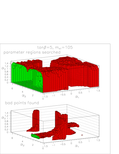
Figure 7: For $\tan\beta=5$ and $m_{h_{1}}=105\,{\rm GeV}$, we display in three dimensional $(\alpha_{1},\alpha_{2},\alpha_{3})$ parameter space the parameter regions searched (which lie within the surfaces shown), and the regions therein for which the remaining model parameters can be chosen so that no Higgs boson is observable (interior to the surfaces shown).

To illustrate, we shall discuss results for $\tan\beta=3$, $\tan\beta=5$ and $\tan\beta=10$ (for which $m_{h_{1}}^{\rm max}\sim 124\,{\rm GeV}$, $118\,{\rm GeV}$ and $114\,{\rm GeV}$, respectively) and $m_{h_{1}}=105\,{\rm GeV}$.

• In Fig. 7, we display for $\tan\beta=5$ both the portions of $(\alpha_{1},\alpha_{2},\alpha_{3})$ parameter space that satisfy our search restrictions, and the regions (termed “regions of unobservability”) within the searched parameter space such that, for some choice of the remaining parameters ($\lambda$ and $m_{a}$), no Higgs boson will be detected using any of the techniques discussed earlier.  Relatively large regions of unobservability within the searched parameter space are present.

• At $\tan\beta=3$, The search region that satisfies our criteria is nearly the same; the regions of unobservability lie mostly within those found for $\tan\beta=5$, and are about 50% smaller.

• For $\tan\beta=10$, the regions of unobservability comprise only a very small portion of those found for $\tan\beta=5$. This reduction is due to the increased $b\overline{b}$ couplings of the $h_{i}$ and $a$, which imply increased $b\overline{b}h_{i},b\overline{b}a$ production cross sections. As these cross sections become large, detection of at least one of the $h_{i}$ and/or the $a$ in the $b\overline{b}\tau^{+}\tau^{-}$ final state becomes increasingly difficult to avoid. For values of $\tan\beta\mathrel{\raise 1.29167pt\hbox{$>$\kern-7.5pt\lower 4.30554pt\hbox{$\sim$}}}10$,  we find that one or more of the $h_{i},a$ should be observable regardless of location in $(\alpha_{1},\alpha_{2},\alpha_{3},\lambda,m_{a})$ parameter space (within the somewhat restricted search region that we explore).

Details of what goes wrong at a typical point are summarized elsewhere. $\!{}^{{\bf?}}$

Supersymmetric decays of the Higgs bosons are neglected in the above. If these decays are important, the regions of unobservability found without using the SUSY final states will increase in size. However, Higgs masses in the regions of unobservability are typically modest in size ($100-200\,{\rm GeV}$), and as SUSY mass limits increase with LEP2 running this additional concern will become less relevant. Of course, if SUSY decays are significant, detection of the Higgs bosons in the SUSY modes might be possible, in which case the regions of unobservability might decrease in size. Assessment of this issue is dependent upon a specific model for soft SUSY breaking.

Although it is not possible to establish a no-lose theorem for the NMSSM Higgs bosons by combining data from LEP2 and the LHC (in contrast to the no-lose theorems applicable to the NLC Higgs search with $\sqrt{s}\mathrel{\raise 1.29167pt\hbox{$>$\kern-7.5pt\lower 4.30554pt\hbox{$\sim$}}}300\,{\rm GeV}$), the regions of complete Higgs boson unobservability appear to constitute a small fraction of the total model parameter space. It would be interesting to see whether or not these regions of unobservability correspond to unnatural choices for the Planck scale supersymmetry-breaking parameters.

3.4 The MSSM at the NLC

In what follows, we shall use NLC language when referring to operation of a lepton-lepton collider at $\sqrt{s}=500\,{\rm GeV}$. The reader should keep in mind that the FMC can also be run in an NLC-like mode. Results for $s$-channel Higgs discovery in the MSSM at the FMC will be summarized separately.

In the MSSM, the important production mechanisms are mainly determined by the parameters $m_{A^{0}}$ and $\tan\beta$. In general, we shall try to phrase our survey in terms of the parameter space defined by $(m_{A^{0}},\tan\beta)$, keeping fixed the other MSSM parameters such as the masses of the top squarks. The most important general point is the complementarity of the $e^{+}e^{-}\rightarrow Zh^{0}$ and $e^{+}e^{-}\rightarrow A^{0}H^{0}$ cross sections, which are proportional to $\sin^{2}(\beta-\alpha)$, and the $e^{+}e^{-}\rightarrow ZH^{0}$ and $e^{+}e^{-}\rightarrow A^{0}h^{0}$ cross sections, proportional to $\cos^{2}(\beta-\alpha)$. (Here, $\alpha$ is the mixing angle that emerges in diagonalizing the CP-even Higgs sector.) Since $\cos^{2}(\beta-\alpha)$ and $\sin^{2}(\beta-\alpha)$ cannot simultaneously be small, if there is sufficient energy then there is a large production cross section for all three of the neutral Higgs bosons. In the more likely case that $m_{A^{0}}$ is large, $\sin^{2}(\beta-\alpha)$ will be large and the $h^{0}$ will be most easily seen in the $Zh^{0}$ channel, while the $A^{0}$ and $H^{0}$ will have a large production rate in the $A^{0}H^{0}$ channel if $\sqrt{s}$ is adequate. If $\cos^{2}(\beta-\alpha)$ is large, then $m_{A^{0}}$ must be small and $A^{0}h^{0}$ and $ZH^{0}$ will have large rates.

Detection of the $h^{0}$

In the MSSM, the lightest Higgs boson is accessible in the $Zh^{0}$ and $WW$-fusion modes for all but the $m_{A^{0}}\leq m_{Z}$, $\tan\beta\geq 7-10$ corner of parameter space. Outside this region the $h^{0}$ rapidly becomes SM-like. A figure illustrating this and detailed discussions can be found in DPF95 $\!{}^{{\bf?}}$ and in many other reviews and reports. $\!{}^{{\bf?},{\bf?},{\bf?},{\bf?},{\bf?},{\bf?}}$ As noted earlier, event rates in the $Zh^{0}$ mode will be sufficient even if the $h^{0}$ decays mostly invisibly to a $\widetilde{\chi}^{0}_{1}\widetilde{\chi}^{0}_{1}$ pair. $\!{}^{{\bf?},{\bf?},{\bf?}}$

If such SUSY decays are not important for the $h^{0}$, then, to a very good approximation, the entire SM discussion can be taken over for $Zh^{0}$ for large $m_{A^{0}}$. As we emphasized earlier, the interesting question becomes for what portion of moderate-$m_{A^{0}}$ parameter space can the cross sections, branching ratios and/or couplings be measured with sufficient precision to distinguish an approximately SM-like $h^{0}$ from the $h_{\rm SM}$ at the NLC and/or FMC. Expectations based on the accuracies tabulated in Tables 10, 11, and 12 were given in Sec. 2.2. The conclusions depend upon whether only NLC data, or both NLC and $s$-channel FMC data, are available. For an NLC running at $\sqrt{s}=500\,{\rm GeV}$ with $L=200~{}{\rm fb}^{-1}$ of integrated luminosity and a vertex tagger good enough to topologically separate $b$ from $c$ jets, we will be able to tell the difference between the $h_{\rm SM}$ and the $h^{0}$ at the $\sim 3\sigma$ level if $m_{A^{0}}\mathrel{\raise 1.29167pt\hbox{$<$\kern-7.5pt\lower 4.30554pt\hbox{$\sim$}}}400\,{\rm GeV}$. If both NLC and $s$-channel FMC data ($L=200~{}{\rm fb}^{-1}$ each) are available, then discrimination between the $h_{\rm SM}$ and the $h^{0}$ at the $3\sigma$ level should be possible up to $m_{A^{0}}\sim 600\,{\rm GeV}$ (based upon the determination of the $\mu^{+}\mu^{-}$ partial width).

Although strongly disfavored by model building and increasingly restricted by LEP2 data, there is still a possibility that $m_{A^{0}}\mathrel{\raise 1.29167pt\hbox{$<$\kern-7.5pt\lower 4.30554pt\hbox{$\sim$}}}m_{Z}$. The important production process will then be $e^{+}e^{-}\rightarrow Z^{\star}\rightarrow h^{0}A^{0}$, the $h^{0}ZZ$ and $h^{0}WW$ couplings being suppressed for such $m_{A^{0}}$ values. Once LEP2 runs at $\sqrt{s}=192\,{\rm GeV}$ $h^{0}A^{0}$ associated production will be kinematically allowed and detectable for all but very large $m_{\widetilde{t}}$ values. The NLC could be run at a $\sqrt{s}$ value optimized for detailed studies of the $h^{0}A^{0}$ final state. At $\sqrt{s}=500\,{\rm GeV}$, at least 1500 events are predicted for precisely the $m_{A^{0}}\mathrel{\raise 1.29167pt\hbox{$<$\kern-7.5pt\lower 4.30554pt\hbox{$\sim$}}}100\,{\rm GeV}$, $\tan\beta\mathrel{\raise 1.29167pt\hbox{$>$\kern-7.5pt\lower 4.30554pt\hbox{$\sim$}}}2-5$ section of parameter space for which fewer events than this would be found in the $Zh^{0}$ mode. Thus, $e^{+}e^{-}\rightarrow h^{0}A^{0}$ will give us a large number of $h^{0}$’s if $Zh^{0}$ does not. In what follows, our focus will be on large $m_{A^{0}}$; we will confine ourselves to a only few general remarks regarding the small-$m_{A^{0}}$ scenario.

Detection of the $H^{0}$, $A^{0}$ and $H^{\pm}$

For $m_{A^{0}}\mathrel{\raise 1.29167pt\hbox{$<$\kern-7.5pt\lower 4.30554pt\hbox{$\sim$}}}m_{Z}$, the $A^{0}$, along with the $h^{0}$, can be easily detected in the $h^{0}A^{0}$ mode, as discussed above. If 50 events are adequate, detection of both the $h^{0}$ and $A^{0}$ in this mode will even be possible for $m_{A^{0}}$ up to $\sim 120\,{\rm GeV}$. In this same region the $H^{0}$ will be found via $ZH^{0}$ and $WW$-fusion production. $\!{}^{{\bf?},{\bf?},{\bf?},{\bf?}}$ In addition, $H^{+}H^{-}$ pair production will be kinematically allowed and easily observable. $\!{}^{{\bf?},{\bf?},{\bf?},{\bf?}}$ In this low to moderate $m_{A^{0}}$ region, the only SUSY decay mode that has a real possibility of being present is the invisible $\widetilde{\chi}^{0}_{1}\widetilde{\chi}^{0}_{1}$ mode for the neutral Higgs bosons. If this mode were to dominate the decays of all three neutral Higgs bosons, then only the $H^{0}$ could be detected, using the recoil mass technique in the $ZH^{0}$ channel. However, in the $H^{+}H^{-}$ channel the final states would probably not include SUSY modes and $H^{+}$ discovery would be straightforward. If a light $H^{\pm}$ is detected, then one would know that the Higgs detected in association with the $Z$ was most likely the $H^{0}$ and not the $h^{0}$. A dedicated search for the light $A^{0}$ and $h^{0}$ through (rare) non-invisible decays would then be appropriate.

For $m_{A^{0}}\geq 120\,{\rm GeV}$, $e^{+}e^{-}\rightarrow H^{0}A^{0}$ and $e^{+}e^{-}\rightarrow H^{+}H^{-}$ must be employed for detection of the three heavy Higgs bosons. Assuming that SUSY decays are not dominant, and using the 50 event criterion, the mode $H^{0}A^{0}$ is observable up to $m_{H^{0}}\sim m_{A^{0}}\sim 240$ GeV, and $H^{+}H^{-}$ can be detected up to $m_{H^{\pm}}=230$ GeV, $\!{}^{{\bf?},{\bf?},{\bf?},{\bf?}}$ assuming $\sqrt{s}=500\,{\rm GeV}$. For $\sqrt{s}_{e^{+}e^{-}}=500\,{\rm GeV}$, the $\gamma\gamma$ collider mode could potentially extend the reach for the $H^{0},A^{0}$ bosons up to 400 GeV, especially if $\tan\beta$ is not large. This is discussed in several places $\!{}^{{\bf?},{\bf?},{\bf?}}$ and will not be reviewed further here.

The upper limits in the $H^{0}A^{0}$ and $H^{+}H^{-}$ modes are almost entirely a function of the machine energy (assuming an appropriately higher integrated luminosity is available at a higher $\sqrt{s}$). Two recent studies $\!{}^{{\bf?},{\bf?}}$ show that at $\sqrt{s}=1$ TeV, with an integrated luminosity of $200~{}{\rm fb}^{-1}$, $H^{0}A^{0}$ and $H^{+}H^{-}$ detection would extend to $m_{H^{0}}\sim m_{A^{0}}\sim m_{H^{\pm}}\sim 450$ GeV even if substantial SUSY decays of these heavier Higgs are present. As frequently noted, models in which the MSSM is implemented in the coupling-constant-unification, radiative-electroweak-symmetry-breaking context often predict masses above 200 GeV, suggesting that this extension in mass reach over that for $\sqrt{s}=500$ GeV might be crucial. If a high luminosity high energy muon collider with $\sqrt{s}\sim 4\,{\rm TeV}$ proves feasible, pair production could be studied for $m_{A^{0}}\sim m_{H^{0}}\sim m_{H^{\pm}}$ as large as $\sim 1.8\,{\rm TeV}$, which certainly would include any reasonable model.

It is crucial that the $H^{0},A^{0},H^{\pm}$ be found if supersymmetric particles are observed. Only in this way can we verify directly that the MSSM Higgs sector includes at least the minimal content required. Once discovered, an important question is how much can be learned from $H^{0}A^{0}$ and $H^{+}H^{-}$ pair production regarding the detailed structure of the MSSM. The recent investigations $\!{}^{{\bf?},{\bf?}}$ indicate that a full study of these pair production final states will place extremely powerful constraints on the GUT boundary conditions underlying the MSSM model. Alternatively, the Higgs studies could reveal inconsistencies between the minimal two-doublet Higgs sector predictions and constraints from direct supersymmetry production studies (for any choice of GUT boundary conditions). Then, searches for additional heavy Higgs would become a priority.

It is useful to illustrate just how powerful the details of $H^{0},A^{0},H^{\pm}$ decays are as a test of the model and for determining the underlying GUT boundary conditions at the GUT/Planck mass scale. In one study, $\!{}^{{\bf?}}$, this has been illustrated by examining six not terribly different GUT-scale boundary condition scenarios in which there is universality for the soft-SUSY-breaking parameters $m_{1/2}$, $m_{0}$ and $A_{0}$ associated with soft gaugino masses, soft scalar masses and soft Yukawa coefficients, respectively. $\!{}^{{\bf?}}$ After requiring that the electroweak symmetry breaking generated as a result of parameter evolution yield the correct $Z$ boson mass, the only other parameters required to fully specify a model in this universal-boundary-condition class are $\tan\beta$ and the sign of the $\mu$ parameter (appearing in the superpotential $W\ni\mu\hat{H}_{1}\hat{H}_{2}$). The six models considered $\!{}^{{\bf?}}$ are denoted D^-, D⁺, NS^-, NS⁺, HS^-, HS⁺, where the superscript indicates ${\rm sign}(\mu)$. Each is specified by a particular choice for $m_{0}:m_{1/2}:A_{0}$, thereby leaving only $m_{1/2}$, in addition to $\tan\beta$, as a free parameter in any given model. Pair production is then considered in the context of each model as a function of location in the kinematically and constraint allowed portion of $(m_{1/2},\tan\beta)$ parameter space.

It is found $\!{}^{{\bf?}}$ that event rates for anticipated machine luminosities are such that $H^{0}A^{0}$ and $H^{+}H^{-}$ pair production can be detected in final state modes where $H^{0},A^{0}\to b\overline{b}$ or $t\overline{t}$ and $H^{+}\to t\overline{b},H^{-}\to b\overline{t}$ even when the branching ratios for SUSY decays are substantial. Further, the mass of the $H^{0}$ or $A^{0}$ can be determined with substantial accuracy using the fully reconstructable all jet final states associated with these modes. Most importantly, in much of the kinematically and phenomenologically allowed parameter space Higgs branching ratios for a variety of different decay channels can be measured by “tagging” one member of the Higgs pair in a fully reconstructable all jet decay mode and then searching for different types of final states in the decay of the second (recoiling) Higgs boson.

The power of Higgs pair observations for determining the GUT boundary conditions is most simply illustrated by an example. Let us suppose that the D^- model with $m_{1/2}=201.7\,{\rm GeV}$ and $\tan\beta=7.5$ is nature’s choice. This implies that $m_{A^{0}}=349.7\,{\rm GeV}$ and $m_{\widetilde{\chi}^{\pm}_{1}}=149.5\,{\rm GeV}$. Experimentally, one would measure $m_{A^{0}}$ as above and $m_{\widetilde{\chi}^{\pm}_{1}}$ (the lightest chargino) mass in the usual way and then infer the required parameters for a given model. For the six models the parameters are given in Table 14. Note that if the correct GUT scenario can be ascertained experimentally, then $\tan\beta$ and $m_{1/2}$ will be fixed.

Table 14: We tabulate the values of $m_{1/2}$ (in GeV) and $\tan\beta$ required in each of our six scenarios in order that $m_{A^{0}}=349.7\,{\rm GeV}$ and $m_{\widetilde{\chi}^{\pm}_{1}}=149.5\,{\rm GeV}$. Also given are the corresponding values of $m_{H^{0}}$. Masses are in GeV.

	D-	D+	NS-	NS+	HS-	HS+
$m_{1/2}$	201.7	174.4	210.6	168.2	203.9	180.0
$\tan\beta$	7.50	2.94	3.24	2.04	12.06	3.83
$m_{H^{0}}$	350.3	355.8	353.9	359.0	350.1	353.2

Determination of the GUT scenario proceeds as follows. Given the parameters required for the observed $m_{A^{0}}$ and $m_{\widetilde{\chi}^{\pm}_{1}}$ for each model, as tabulated in Table 14, the rates for different final states of the recoil (non-tagged) Higgs boson in pair production can be computed. Those for the input D^- model are used to determine the statistical accuracy with which ratios of event numbers in different types of final states can be measured.  The ratios predicted in the D⁺, NS^-, NS⁺, HS^-, and HS⁺models will be different from those predicted for the input D^- model. Thus, the statistical uncertainty predicted for the various ratios in the input D^- model can be used to compute the $\chi^{2}$ by which the predictions of the other models differ from the central values of the input D^- model. The results for a selection of final state ratios are given in Table 15. The final states considered are: $b\overline{b}$ and $t\overline{t}$ for the $H^{0},A^{0}$; $h^{0}h^{0}$ (light Higgs pair, with $h^{0}\to b\overline{b}$) for the $H^{0}$; $h^{0}W^{+}$ and $\tau^{+}\nu_{\tau}$ for the $H^{+}$ (or the charge conjugates for the $H^{-}$); and SUSY modes (experimentally easily identified by the presence of missing energy) classified according to the number of charged leptons summed over any number of jets (including 0). All branching ratios and reasonable efficiencies are incorporated in the statistical errors employed in constructing this table. The effective luminosity $L_{\rm eff}=80~{}{\rm fb}^{-1}$ is equivalent to an overall tagging and reconstruction efficiency for events of $\epsilon=0.4$ at a total integrated luminosity of $L=200~{}{\rm fb}^{-1}$. Results presented are for $\sqrt{s}=1\,{\rm TeV}$.

Table 15: We tabulate $\Delta\chi^{2}_{i}$ (relative to the D^- scenario) for the indicated branching fraction ratios as a function of scenario, assuming the measured $m_{A^{0}}$ and $m_{\widetilde{\chi}^{\pm}_{1}}$ values are $349.7\,{\rm GeV}$ and $149.5\,{\rm GeV}$, respectively. The SUSY channels have been resolved into final states involving a fixed number of leptons. The error used in calculating each $\Delta\chi^{2}_{i}$ is the approximate $1\sigma$ error with which the given ratio could be measured for $L_{\rm eff}=80~{}{\rm fb}^{-1}$ at $\sqrt{s}=1\,{\rm TeV}$ assuming that the D^- scenario is the correct one.

Ratio	D+	NS-	NS+	HS-	HS+
$\langle H^{0},A^{0}\rangle$
$[0\ell][\geq 0j]/b\overline{b},t\overline{t}$	12878	1277	25243	0.77	10331
$[1\ell][\geq 0j]/b\overline{b},t\overline{t}$	13081	2.41	5130	3.6	4783
$[2\ell][\geq 0j]/b\overline{b},t\overline{t}$	4543	5.12	92395	26.6	116
$h^{0}h^{0}/b\overline{b}$	109	1130	1516	10.2	6.2
$H^{+}$
$[0\ell][\geq 0j]/t\overline{b}$	12.2	36.5	43.2	0.04	0.2
$[1\ell][\geq 0j]/t\overline{b}$	1.5	0.3	0.1	5.6	0.06
$h^{0}W/t\overline{b}$	0.8	0.5	3.6	7.3	0.3
$\tau\nu/t\overline{b}$	43.7	41.5	47.7	13.7	35.5
$\sum_{i}\Delta\chi^{2}_{i}$	30669	2493	124379	68	15272

From Table 15 it is clear that the five alternative models can be discriminated against at a high (often very high) level of confidence. Further subdivision of the SUSY final states into states containing a certain number of jets yields even more discrimination power. $\!{}^{{\bf?}}$ Thus, not only will detection of Higgs pair production in $e^{+}e^{-}$ or $\mu^{+}\mu^{-}$ collisions (at planned luminosities) be possible for most of the kinematically accessible portion of parameter space in a typical GUT model, but also the detailed rates for and ratios of different neutral and charged Higgs decay final states will very strongly constrain the possible GUT-scale boundary condition scenario and choice of parameters, e.g. $\tan\beta$ and $m_{1/2}$, therein.

3.5 The MSSM in $s$-channel collisions at the FMC

We have seen that other colliders offer various mechanisms to directly search for the $A^{0},H^{0}$, but have significant limitations:

• The LHC has “$h^{0}$-only” regions at moderate $\tan\beta$, $m_{A^{0}}\geq 200\,{\rm GeV}$.

• At the NLC one can use the mode $e^{+}e^{-}\to Z^{\star}\to H^{0}A^{0}$ (the mode $h^{0}A^{0}$ is suppressed for large $m_{A^{0}}$), but it is limited to $m_{H^{0}}\sim m_{A^{0}}\mathrel{\raise 1.29167pt\hbox{$<$\kern-7.5pt\lower 4.30554pt\hbox{$\sim$}}}\sqrt{s}/2$.

• A $\gamma\gamma$ collider could probe heavy Higgs up to masses of $m_{H^{0}}\sim m_{A^{0}}\sim 0.8\sqrt{s}_{e^{+}e^{-}}$, but this would quite likely require $L\sim 100-200{~{}{\rm fb}}^{-1}$, especially if the Higgs bosons have masses near $400\,{\rm GeV}$ and $\tan\beta$ is large. $\!{}^{{\bf?},{\bf?},{\bf?}}$

In contrast, there is an excellent chance of being able to detect the $H^{0},A^{0}$ at a $\mu^{+}\mu^{-}$ collider provided only that $m_{A^{0}}$ is smaller than the maximal $\sqrt{s}$ available. This could prove to be very important given that GUT MSSM models usually predict $m_{A^{0}}>200\,{\rm GeV}$.

A detailed study of $s$-channel production of the $H^{0},A^{0}$ has been made. $\!{}^{{\bf?}}$ The optimal strategy for their detection and study depends upon the circumstances. First, it could be that the $H^{0}$ and/or $A^{0}$ will already have been discovered at the LHC. With $L=300~{}{\rm fb}^{-1}$ of integrated luminosity for ATLAS and CMS (each), this would be the case if $\tan\beta\leq 3$ (or $\tan\beta$ is large); see Fig. 5. Even if the $H^{0},A^{0}$ have not been detected, then, as described earlier, strong constraints on $m_{A^{0}}$ are possible through precision measurements of the properties of the $h^{0}$ at the NLC and/or FMC. For example, if no deviation is observed at the NLC in $L=200~{}{\rm fb}^{-1}$ running at $\sqrt{s}=500\,{\rm GeV}$, then we would know that $m_{A^{0}}>400\,{\rm GeV}$. If a statistically significant deviation from SM predictions is observed, then an approximate determination of $m_{A^{0}}$ would be possible. Either way, we could limit the $\sqrt{s}$ scan for the $A^{0}$ in the $s$-channel to the appropriate mass region and thereby greatly facilitate direct observation of the $A^{0}$ and $H^{0}$ since it would allow us to devote more luminosity per scan point than if $m_{A^{0}}$ is not constrained.

With such pre-knowledge of $m_{A^{0}}$, it will be possible to detect and perform detailed studies of the $H^{0},A^{0}$ for essentially all $\tan\beta\geq 1$ provided only that $m_{A^{0}}\leq\sqrt{s}_{\rm max}$.  If $\tan\beta\leq 3$, then excellent resolution, $R\sim 0.01\%$, will be necessary for detection since the $A^{0}$ and $H^{0}$ become relatively narrow for low $\tan\beta$ values. For higher $\tan\beta$ values $R\sim 0.1\%$ is adequate for $H^{0},A^{0}$ detection, but $R\sim 0.01\%$ would be required in order to separate the rather degenerate $H^{0}$ and $A^{0}$ peaks (as a function of $\sqrt{s}$) from one another.

Even without pre-knowledge of $m_{A^{0}}$, there would be an excellent chance for discovery of the $A^{0},H^{0}$ Higgs bosons in the $s$-channel at a $\mu^{+}\mu^{-}$ collider if they have not already been observed at the LHC, given that the latter implies that $\tan\beta>3$. Indeed, detection of the $A^{0},H^{0}$ is possible $\!{}^{{\bf?}}$ in the mass range from 200 to 500 GeV via a $s$-channel scan in $\mu^{+}\mu^{-}$ collisions provided $\tan\beta\geq 3$ and $L=200~{}{\rm fb}^{-1}$ of luminosity is devoted to the scan. (A detailed strategy as to how much luminosity to devote to different $\sqrt{s}$ values in the $200-500\,{\rm GeV}$ range during this scan must be employed. $\!{}^{{\bf?}}$) That the signals become viable when $\tan\beta>1$ (as favored by GUT models) is due to the fact that the couplings of $A^{0}$ and (once $m_{A^{0}}\geq 150\,{\rm GeV}$) $H^{0}$ to $b\overline{b}$ and, especially to $\mu^{+}\mu^{-}$, are proportional to $\tan\beta$, and thus increasingly enhanced as $\tan\beta$ rises. In the $\tan\beta\geq 3$ region, a beam energy resolution of $R\mathrel{\raise 1.29167pt\hbox{$<$\kern-7.5pt\lower 4.30554pt\hbox{$\sim$}}}0.1\%$ is adequate for the scan to be successful in discovery, but as already noted $R\sim 0.01\%$ is needed to separate the $H^{0}$ and $A^{0}$ peaks from one another. That the LHC and the FMC are complementary in this respect is a very crucial point. Together, the LHC and FMC essentially guarantee discovery of the $A^{0},H^{0}$ so long as they have masses less than the maximum $\sqrt{s}$ of the FMC.

In the event that the NLC has not been constructed, it could be that the first mode of operation of the FMC would be to optimize for and accumulate luminosity at $\sqrt{s}=500\,{\rm GeV}$ (or whatever the maximal value is). In this case, there is still a significant chance for detecting the $H^{0},A^{0}$ even if $m_{A^{0}}\geq\sqrt{s}/2$. Although reduced in magnitude compared to an electron collider, there is a long low-energy bremsstrahlung tail at a muon collider that provides a self-scan over the range of energies below the design energy, and thus can be used to detect $s$-channel resonances. Observation of $A^{0},H^{0}$ peaks in the $b\overline{b}$ mass distribution $m_{b\overline{b}}$ created by this bremsstrahlung tail may be possible. The region of the $(m_{A^{0}},\tan\beta)$ parameter space plane for which a peak is observable depends strongly on the $b\overline{b}$ invariant mass resolution. For an excellent $m_{b\overline{b}}$ mass resolution of order $\pm 5\,{\rm GeV}$ and integrated luminosity of $L=50~{}{\rm fb}^{-1}$ ($200~{}{\rm fb}^{-1}$) at $\sqrt{s}=500\,{\rm GeV}$, the $A^{0},H^{0}$ peak(s) are observable for $\tan\beta\geq 5-6$ ($3.5-4.5$) if $250\,{\rm GeV}\leq m_{A^{0}}\leq 500\,{\rm GeV}$ — i.e. the LHC/FMC gap for $\tan\beta\mathrel{\raise 1.29167pt\hbox{$>$\kern-7.5pt\lower 4.30554pt\hbox{$\sim$}}}3$ is essentially closed at the higher luminosity.

Finally, even if a $\sqrt{s}\sim 500\,{\rm GeV}$ muon collider does not have sufficient energy to discover heavy supersymmetric Higgs bosons in the $s$-channel, construction of a higher energy machine would be possible; a popular reference design is one for $\sqrt{s}=4\,{\rm TeV}$. Such an energy would allow discovery of $\mu^{+}\mu^{-}\to A^{0}H^{0}$ and $H^{+}H^{-}$ pair production, via the $b\overline{b}$ or $t\overline{t}$ decay channels of the $H^{0},A^{0}$ and $t\overline{b},\overline{t}b$ decay channels of the $H^{+},H^{-}$, up to masses very close to $m_{A^{0}}\sim m_{H^{0}}\sim m_{H^{\pm}}\sim 2\,{\rm TeV}$. $\!{}^{{\bf?}}$

3.6 The NMSSM at the NLC

Consider a CP-conserving Higgs sector for the NMSSM, and the three CP-even Higgs bosons $h_{1,2,3}$, labelled in order of increasing mass. The first question is whether or not a $\sqrt{s}=500\,{\rm GeV}$ $e^{+}e^{-}$ collider would still be guaranteed to discover at least one of the NMSSM Higgs bosons. We have seen that in the MSSM there is such a guarantee because the $h^{0}$ has an upper mass bound, and because it has near maximal $h^{0}ZZ$ coupling when $m_{h^{0}}$ approaches its upper limit. In the NMSSM model, it is in principle possible to choose parameters such that $h_{1,2}$ have such suppressed $ZZ$ coupling strength that their $Zh_{1,2}$ and $WW\rightarrow h_{1,2}$ production rates are too low for observation, while the heavier $h_{3}$ Higgs is too heavy to be produced in the $Zh_{3}$ or $WW\rightarrow h_{3}$ modes. This issue has been studied recently. $\!{}^{{\bf?},{\bf?},{\bf?},{\bf?},{\bf?}}$ If the model is placed within the normal unification context, with simple boundary conditions at $M_{X}$, and if all couplings are required to remain perturbative in evolving up to scale $M_{X}$ (as is conventional), then it is found that the above situation does not arise. At least one of the three neutral scalars will have $\sigma(e^{+}e^{-}\rightarrow Zh)\mathrel{\raise 1.29167pt\hbox{$>$\kern-7.5pt\lower 4.30554pt\hbox{$\sim$}}}0.04~{}{\rm pb}$ for any $e^{+}e^{-}$ collider with $\sqrt{s}\geq 300\,{\rm GeV}$. For $L=10~{}{\rm fb}^{-1}$, this corresponds to roughly 30 events in the clean $Zh$ with $Z\rightarrow\ell^{+}\ell^{-}$ recoil-mass discovery mode. However, these same studies all make it clear that there is no guarantee that LEP2 will detect a Higgs boson of the NMSSM. This is because the Higgs boson with significant $ZZ$-Higgs coupling can easily have mass beyond the kinematical reach of LEP2. Of course, once a neutral Higgs bosons is discovered, it will be crucial to measure all its couplings and to determine its CP character (using techniques discussed earlier), not only to try to rule out the possibility that it is the SM $h_{\rm SM}$, but also to try to determine whether or not the supersymmetric model is the MSSM or the NMSSM (or still further extension).

3.7 The NMSSM in $s$-channel collisions at the FMC

This interesting topic is currently under investigation. Unlike the standard $\sqrt{s}=500\,{\rm GeV}$ modes for discovery, the sensitivity in the $s$-channel depends significantly on the $\mu^{+}\mu^{-}$ couplings of the various Higgs bosons.

4 Conclusions

Models in which electroweak symmetry breaking occurs via a Higgs sector, leaving behind physical spin-0 Higgs bosons, continue to be very attractive and imply a rich phenomenology. Our focus has been on supersymmetric theories, in which context Higgs bosons are completely natural and the Higgs sector is highly constrained. Not only must the Higgs sector consist of just two doublets (and no more, and no triplets, unless intermediate scale matter is introduced to fix up coupling unification) plus possible singlets, but also the Higgs sector couplings are closely related to gauge couplings. As a result, there is a strong upper bound on the mass of the lightest CP-even Higgs boson ($h^{0}$) in a supersymmetric model. Further, in the decoupling limit (e.g. for large $m_{A^{0}}$ in the MSSM), the $h^{0}$ becomes SM-like. Thus, Higgs phenomenology for the simpler supersymmetric models is relatively well defined. This review has outlined the more important highlights regarding experimentally probing a supersymmetric Higgs sector at the LHC, NLC and FMC colliders. Some principle points and conclusions include the following.

• In the minimal two-doublet/no-singlet MSSM model, discovery of at least one Higgs boson is guaranteed both at the LHC and in Higgstrahlung or Higgs pair production at a $\sqrt{s}\geq 300\,{\rm GeV}$ NLC and/or FMC, regardless of $m_{A^{0}}$. For large $m_{A^{0}}$, it is the SM-like $h^{0}$ that would be observed. Since $m_{h^{0}}<2m_{W}$, the SM-like $h^{0}$ could also be produced at a high rate in $s$-channel collisions at the FMC.

• In the two-doublet/one-singlet NMSSM model, discovery of at least one Higgs boson is certain at the NLC and/or FMC, but can no longer be absolutely guaranteed at the LHC (although it is highly probable).

• Precision determination of all the couplings, the total width and the mass of a light SM-like Higgs boson will be possible. The LHC and NLC often provide highly complementary information. For example, in the MSSM-preferred $\leq 130\,{\rm GeV}$ mass range, data from the LHC, from $e^{+}e^{-}$ collisions at the NLC (or $\mu^{+}\mu^{-}$ collisions at the FMC) and from $\gamma\gamma$ collisions at the NLC are all necessary in order to extract the absolute coupling magnitudes and the total width with good precision in a model-independent way. Production in the $s$-channel at the FMC would provide additional precision measurements of relative branching ratios and a direct measurement of the total width. Such precision measurements could make it possible to distinguish a SM-like $h^{0}$ of the MSSM from the SM $h_{\rm SM}$.

• Thus, if the light $h^{0}$ of the supersymmetric models is SM-like, it would be enormously advantageous to have, in addition to the LHC and an NLC operating at $\sqrt{s}\sim 500\,{\rm GeV}$, an FMC concentrating on $s$-channel Higgs studies. All three facilities are needed in order to maximize the precision with which the properties of a light SM-like Higgs boson can be determined. The value of the resulting precision is great. If $L=200~{}{\rm fb}^{-1}$ of data is accumulated both in NLC running at $\sqrt{s}=500\,{\rm GeV}$ and in $s$-channel production at the FMC, then $h^{0}$ vs. $h_{\rm SM}$ discrimination is possible at the $\geq 3\sigma$ level for $m_{A^{0}}\leq 600\,{\rm GeV}$, and $m_{A^{0}}$ can be determined to within $\sim\pm 50\,{\rm GeV}$.

• Prospects for discovery of the heavier, non-SM-like $H^{0},A^{0}$ of the MSSM are excellent. They will be found at the LHC if $m_{A^{0}}\leq 200\,{\rm GeV}$ or at higher $m_{A^{0}}$ if either $\tan\beta\leq 3$ or $\tan\beta$ is large. If they are not found at the LHC, then the resulting limits on $m_{A^{0}}$ and $\tan\beta$ tell us how to distribute the luminosity of a $L=200~{}{\rm fb}^{-1}$ $s$-channel scan at the FMC so as to guarantee their discovery (if $m_{A^{0}}\leq 500\,{\rm GeV}$). Even if the FMC is run at maximal $\sqrt{s}$, discovery of the $H^{0},A^{0}$ is still possible for $m_{A^{0}}$ below $\sqrt{s}$ if $\tan\beta$ is large; peaks in the $b\overline{b}$ mass distribution, deriving from $s$-channel production via the bremstrahlung tail in the $\mu^{+}\mu^{-}$ energy spectrum, would be visible. Discovery of the $H^{0},A^{0}$ in the $\gamma\gamma$ collider mode of operation at the NLC is possible if $m_{A^{0}}\leq 0.8\sqrt{s}$ and integrated luminosity of $L\geq 100-200~{}{\rm fb}^{-1}$ is accumulated. At the NLC or FMC, $H^{0}A^{0}$ and $H^{+}H^{-}$ pair production will be observable provided $\sqrt{s}>2m_{A^{0}}$. Once discovered, detailed studies of the decays of the $H^{0}$, $A^{0}$ and $H^{\pm}$ would be possible and would strongly constrain the GUT-scale soft-supersymmetry-breaking parameters.

To summarize, if Higgs bosons exist, they are very likely to be part of a supersymmetric theory, and experimental efforts directed towards fully studying the Higgs bosons will provide one of the most exciting programs at the next generation of colliders. Substantial progress has been made in detailing the strategies required at the different accelerators for the discovery and study of the Higgs bosons of a supersymmetric model Higgs sector.

References

References

- [1] A. Blondel, this volume.
- [2] For a review and early references, see: J.F. Gunion, H.E. Haber, G. Kane and S. Dawson, The Higgs Hunters Guide (Addison-Wesley Publishing Company, Redwood City, CA, 1990).
- [3] J.F. Gunion, L. Poggioli and R. Van Kooten, to appear in the Proceedings of the 1996 DPF/DPB Summer Study on New Directions for High-Energy Physics, denoted by Snowmass 96 in subsequent references.
- [4] H.E. Haber, this volume.
- [5] S. Pokorski, this volume.
- [6] J. Ellis, J.F. Gunion, H.E. Haber, L. Roszkowski and F. Zwirner, Phys. Rev. D 39, 844 (1989).
- [7] J.F. Gunion, A. Stange, and S. Willenbrock, Weakly-Coupled Higgs Bosons, preprint UCD-95-28 (1995), to be published in Electroweak Physics and Beyond the Standard Model, World Scientific Publishing Co., eds. T. Barklow, S. Dawson, H. Haber, and J. Siegrist.
- [8] Physics and Technology of the Next Linear Collider: a Report Submitted to Snowmass 1996, BNL 52-502, FNAL-PUB-96/112, LBNL-PUB-5425, SLAC Report 485, UCRL-ID-124160.
- [9] V. Barger, M. Berger, J.F. Gunion and T. Han, UCD-96-6 (hep-ph/9602415, January, 1996), to appear in Physics Reports.
- [10] M. Carena et al., CERN-96-01 (hep-ph/9602250).
- [11] A. Djouadi et al., hep-ph/9605437
- [12] S. Mrenna, this volume.
- [13] S. Kim, S. Kuhlmann, W.-M. Yao, Snowmass 96.
- [14] W.-M. Yao, Snowmass 96.
- [15] E.W.N. Glover, J. Ohnemus, and S. Willenbrock, Phys. Rev. D 37, 3193 (1988).
- [16] V. Barger, G. Bhattacharya, T. Han and B. Kniehl, Phys. Rev. D 43, 779 (1991).
- [17] M. Dittmar and H. Dreiner, hep-ph/9608317.
- [18] L. Poggioli, preliminary communication regarding a study being performed by the ATLAS collaboration.
- [19] J.F. Gunion and R. Van Kooten, work performed for Snowmass 96.
- [20] Based on work performed by J.F. Gunion.
- [21] S. Narison, Phys. Lett. B 341, 73 (1994); for a review, see S. Narison, hep-ph/9510270, presented at the 1995 Europhysics Conference on High Energy Physics, Brussels, Belgium, July 27-31, 1995.
- [22] J. Shigemitsu, talk presented at the Aspen Winter Conference on High Energy Physics, Aspen, January 1997.
- [23] A. Djouadi, talk presented at the workshop on “The Higgs Puzzle”, Ringberg, Germany, December 1996, hep-ph/970320.
- [24] See p. 25 of the NLC report.
- [25] J.F. Gunion and P. Martin, Snowmass 96; and UCD-96-15 (hep-ph/9607360).
- [26] J.F. Gunion, T. Han and R. Sobey, UCD-97-01, in preparation.
- [27] J.F. Gunion and H.E. Haber, Phys. Rev. D 48, 5109 (1993).
- [28] D. Borden, D. Bauer, and D. Caldwell, Phys. Rev. D 48, 4018 (1993).
- [29] V. Barger, M. Berger, J.F. Gunion and T. Han, work in progress.
- [30] P. Janot, private communication.
- [31] V. Barger, M. Berger, J.F. Gunion and T. Han, preprint UCD-96-39 (hep-ph/9612279, 1996).
- [32] M. Kramer, J. Kuhn, M. Stong, and P. Zerwas, Z. Phys. C 64, 21 (1994).
- [33] J.F. Gunion and B. Grzadkowski, Phys. Lett. B 350, 218 (1995).
- [34] J.F. Gunion and X.G. He, Phys. Rev. Lett. 76, 4468 (1996).
- [35] J.F. Gunion, T.C. Yuan and B. Grzadkowski, Phys. Rev. Lett. 71, 488 (1993).
- [36] J. F. Gunion, B. Grzadkowski and X.-G. He, Phys. Rev. Lett. 77, 5172 (1996).
- [37] J.F. Gunion and X.-G. He, Snowmass 96.
- [38] J.F. Gunion and B. Grzadkowski, Phys. Lett. B 294, 361 (1992).
- [39] J.F. Gunion and J. Kelly, Phys. Lett. B 333, 110 (1994).
- [40] G.L. Kotkin and V.G. Serbo, hep-ph/9611345.
- [41] D. Atwood and A. Soni, Phys. Rev. D 52, 6271 (1995).
- [42] J.F. Gunion, Perspectives on Higgs Physics, ed. G. Kane (World Scientific Publishing), 1st edition, p. 179.
- [43] J. Gunion, in Properties of SUSY Particles, Proceedings of the 23rd Workshop of the INFN Eloisatron Project, Erice, Italy, Sept. 28 - Oct. 4 1992, eds. L. Cifarelli and V. Khoze, p. 279.
- [44] A. Djouadi, J. Kalinowski and P.M. Zerwas, Z. Phys. C 70, 435 (1996).
- [45] Z. Kunszt, S. Moretti and W.J. Stirling, DFFT-34-95 (hep-ph/9611397).
- [46] A. Bartl, H. Eberl, K. Hidaka, T. Kon, W. Majerotto and Y. Yamada, UWTHPH-1997-03 (hep-ph/9701398).
- [47] A. Djouadi, J. Kalinowski and M. Spira, DESY-97-079 (hep-ph/9704448).
- [48] Z. Kunszt and F. Zwirner, Nucl. Phys. B 385, 3 (1992).
- [49] H. Baer, M. Bisset, C. Kao, and X. Tata, Phys. Rev. D 46, 1067 (1992); H. Baer, M. Bisset, D. Dicus, C. Kao, and X. Tata, Phys. Rev. D 47, 1062 (1993).
- [50] J. Gunion and L. Orr, Phys. Rev. D 46, 2052 (1992).
- [51] V. Barger, K. Cheung, R. Phillips, and A. Stange, Phys. Rev. D 46, 4914 (1992).
- [52] F. Gianotti, Proceedings of the European Physical Society International Europhysics Conference on High Energy Physics, Brussels, Belgium, July 27 - August 2, 1995, eds. J. Lemonne, C. Vander Velde and F. Verbeure (World Scientific Publishing), p. 201.
- [53] D. Froidevaux, F. Gianotti, L. Poggioli, E. Richter-Was, D. Cavalli, and S. Resconi, ATLAS Internal Note, PHYS-No-74 (1995).
- [54] P. Janot, this volume.
- [55] D. Dicus and S. Willenbrock, Phys. Rev. D 39, 751 (1989).
- [56] J. Dai, J. Gunion, and R. Vega, Phys. Rev. Lett. 71, 2699 (1993).
- [57] A. Stange, W. Marciano, and S. Willenbrock, Phys. Rev. D 50, 4491 (1994).
- [58] J.F. Gunion, Phys. Lett. B 261, 510 (1991).
- [59] J. Dai, J. Gunion, and R. Vega, Phys. Lett. B 315, 355 (1993).
- [60] J. Dai, J. Gunion, and R. Vega, Phys. Lett. B 345, 29 (1995).
- [61] J. Dai, J. Gunion, and R. Vega, Phys. Lett. B 387, 801 (1996).
- [62] J. Gunion, Phys. Lett. B 322, 125 (1994); V. Barger, R. Phillips, and D. Roy, Phys. Lett. B 324, 236 (1994).
- [63] J. Dai, J. Gunion, and R. Vega, Phys. Lett. B 371, 71 (1996).
- [64] J. Gunion, Phys. Rev. Lett. 72, 199 (1994).
- [65] S.G. Frederiksen, N. Johnson, G. Kane, Phys. Rev. D 50, 4244 (1994).
- [66] D. Choudhury, D.P. Roy, Phys. Lett. B 322, 368 (1994).
- [67] I. Hinchliffe, F.E. Paige, M.D. Shapiro, J. Soderqvist and W. Yao, Phys. Rev. D 55, 5520 (1997).
- [68] J.F. Gunion, H.E. Haber, and T. Moroi, Snowmass 96.
- [69] B.R. Kim, S.K. Oh and A. Stephan, Proceedings of the 2nd International Workshop on “Physics and Experiments with Linear Colliders”, eds. F. Harris, S. Olsen, S. Pakvasa and X. Tata, Waikoloa, HI (1993), World Scientific Publishing, p. 860.
- [70] J. Kamoshita, Y. Okada and M. Tanaka, Phys. Lett. B 328, 67 (1994).
- [71] S.F. King and P.L. White, preprint SHEP-95-27 (1995).
- [72] U. Ellwanger, M.R. de Traubenberg and C.A. Savoy, Z. Phys. C 67, 665 (1995).
- [73] A. Brignole, J. Ellis, J.F. Gunion, M. Guzzo, F. Olness, G. Ridolfi, L. Roszkowski and F. Zwirner, in Collisions at 500 GeV: The Physics Potential, Munich, Annecy, Hamburg Workshop, DESY 92-123A, DESY 92-123B, DESY 93-123C, ed. P. Zerwas, p. 613; A. Djouadi, J. Kalinowski, P.M. Zerwas, ibid., p. 83 and Z. Phys. C 57, 56 (1993); and references therein.
- [74] P. Janot, in ‘92 Electroweak Interactions and Unified Theories, Proceedings of the XXVII Rencontre de Moriond, edited by J. Trân Thanh Vân (Éditions Frontières, Gif-sur-Yvette, 1992), p. 317.
- [75] P. Janot, Proceedings of the 2nd International Workshop on “Physics and Experiments with Linear Colliders”, eds. F. Harris, S. Olsen, S. Pakvasa and X. Tata, Waikoloa, HI (1993), World Scientific Publishing, p. 192; and references therein.
- [76] For an overview, see J.F. Gunion, Proceedings of the 2nd International Workshop on “Physics and Experiments with Linear Colliders”, eds. F. Harris, S. Olsen, S. Pakvasa and X. Tata, Waikoloa, HI (1993), World Scientific Publishing, p. 166.
- [77] J.F. Gunion and J. Kelly, hep/ph-9610421, to appear in the Proceedings of the 1996 DPF/DPB Summer Study on New Directions for High-Energy Physics; detailed results appear in preprint hep/ph-9610495.
- [78] J. Feng and T. Moroi, hep/ph-9612333.
- [79] Definitions of these parameters and discussion of universality can be found in the Snowmass 96 SUSY working group reports: J. Amundsen et al., hep-ph/9609374; and G. Anderson, C.-H. Chen, J.F. Gunion, J. Lykken, T. Moroi and Y. Yamada, UCD-96-25 (hep-ph/9609547).