Condensates and Vacuum Structure of Adjoint $QCD_{2}$

T. Fugleberg, I. Halperin and A. Zhitnitsky

Department of Physics and Astronomy, University of British Columbia, 6224 Agricultural Road, Vancouver, BC, V6T 1Z1, Canada

We discuss a two dimensional $SU(N)$ Yang-Mills theory coupled to massive adjoint fermions for different worlds classified by the integer $k=0,1,...N-1$. We study the fermion condensate for these unconnected worlds as a function of the parameter $k$. We show that the condensate as well as the spectrum of the theory do depend on this vacuum parameter $k$.

Technically, the value of the fermion condensate is related to the value of the gluon condensate via the Operator Product Expansion. We use this to find the leading dependence (in the limit of a heavy quark) of the fermion condensate $\langle k|\bar{\psi}\psi|k\rangle$ on the nontrivial vacuum angle $k$. We also determine the gluon condensate of the theory using low-energy theorems.

1 Introduction

Two dimensional $SU(N)$ Yang Mills theories coupled to adjoint fermions continue to attract theorists [1]-[11] in view of their interesting connections with both string theory on one side and real four dimensional $QCD$ on the other. In particular, as in the latter, $QCD_{2}$ with adjoint matter is expected to possess a nonvanishing fermion condensate $\langle\bar{\psi}\psi\rangle$. This corresponds to a nontrivial vacuum structure of the theory. It is also believed that such a structure is a consequence of nontrivial topological properties of the group $SU(N)/Z_{N}$, which is the relevant symmetry group when adjoint matter (rather than fundamental matter) is considered. Therefore, it is expected that the theory possesses a nontrivial vacuum angle $k$ [12], similar to the $\theta$ angle of QCD. It is known that many problems such as the $U(1)$ problem, chiral symmetry breaking phenomenon, confinement and multiplicity of vacuum states are related to each other and to $\theta$ dependence. Therefore, in spite of the fact that we live in a certain vacuum state (this is expressed by the so-called superselection rule), the physical parameters of the theory do depend on $\theta$, which is an extremely important characteristic of the theory.

The main goal of the present paper is an analysis of the condensate $\langle k|\bar{\psi}\psi|k\rangle$ as a function of the discrete topological vacuum angle label $k=0,1,...N-1$. This dependence can be found explicitly as we shall see. Therefore, the vacuum condensate could be considered as an order parameter which distinguishes different vacuum states.

First we would like to give a short historical introduction of the subject. For the case of fundamental fermions in the large N limit (’t Hooft model [13]) and vanishing fermion mass, the fermion condensate was first calculated in [14]. Later on, the quark condensate was calculated in several different ways, both analytically and numerically [15][16][17].

In the case of adjoint fermions, using bosonization it has been argued [2] that the condensate arises for arbitrary N. At the same time, instanton calculations seem to imply the vanishing of the condensate in the chiral limit for $N\geq 3$. An independent argument, based on quark-hadron duality, has been given to support a nonzero value for the condensate in the large N limit[4]. On the formal side, in the small volume limit the condensate was calculated for $SU(2)$ and $SU(3)$ gauge groups using ET quantization [3]. Similar calculations have been performed for the $SU(2)$ theory in finite volume $L$ using light cone quantization (see [8] [9]). In all finite volume calculations the value of the condensate appears to scale as $\frac{1}{L}$, where L is the quantization volume. Therefore, no continuum limit can be taken in these formulae, and no finite result can be obtained. However, it is believed that an extra factor of $L$ will appear in a complete theory leading to a finite value for the condensate as in the Schwinger model [9] [10]. Unfortunately, this would require a complete solution of the problem which is not possible at present and thus the question regarding the magnitude of the condensate in the continuum limit can not be answered within this approach at the moment.

We conclude this short historical introduction by emphasizing that no meaningful calculation for the quark condensate is hitherto available in the continuum limit for two dimensional $QCD$ with adjoint matter. Therefore, discussion of the number of different vacuum states which is based on the presumption of a nonzero value for the quark condensate has no solid basis before a finite value for the condensate (as an order parameter) is obtained.

Before proceeding we should give a definition of the quark condensate in the theory. We define the fermion condensate in PCAC terms[18] :

$$0 = \lim_{q\rightarrow 0}iq^{\mu}\int d^{2}xe^{iqx}\langle 0|T\{\bar{\psi}\gamma_{\mu}\gamma_{5}\psi(x)\bar{\psi}i\gamma_{5}\psi(0)|0\rangle$$ (1)

$$= 2i\langle 0|\bar{\psi}\psi|0\rangle-2m\int d^{2}x\langle 0|T\{\bar{\psi}i\gamma_{5}\psi(x)\bar{\psi}i\gamma_{5}\psi(0)|0\rangle.$$

This is the standard nonperturbative definition of the quark condensate in terms of the original $\psi$ fields. In particular, in the chiral limit $m\rightarrow 0$, only a Goldstone boson with a finite (at $m\rightarrow 0$) residue $\langle 0|\bar{\psi}i\gamma_{5}\psi(x)|\pi\rangle=i\frac{f_{\pi}m_{\pi}^{2}}{2m}$ contributes to the correlation function $\langle 0|T\{\bar{\psi}i\gamma_{5}\psi(x)\bar{\psi}i\gamma_{5}\psi(0)|0\rangle$. In this case eq.(1) gives the famous relation $m_{\pi}^{2}f_{\pi}^{2}=-4m\langle 0|\bar{\psi}\psi|0\rangle$ between the mass of the Goldstone $\pi$ meson and the chiral condensate.

We want to emphasize that relation (1) is valid not only in the chiral limit $m\rightarrow 0$, but is also satisfied for arbitrary $m$. We expect, of course, that at large $m\rightarrow\infty$ the condensate goes to zero like $\langle 0|\bar{\psi}\psi|0\rangle\sim\frac{1}{m}$.

Nevertheless, a small, but not exactly vanishing condensate will play its role: it will be an order parameter which labels the different vacuum states $|k\rangle$ we have been talking about. This is the cornerstone of our approach. We shall calculate the fermion condensate in the limit of large mass and we shall find different magnitudes for different $|k\rangle$. Presumably a calculation at large $m$ corresponds to the weak coupling regime. Therefore, a perturbative calculation is justified. At the same time the small non-vanishing condensate is sensitive to the particular $|k\rangle$-vacuum state and has a different value for each vacuum state.

As the first step in this program, we shall test our conjecture in the ’t Hooft model [13]. This model is well understood in the limit of large $N$. We know the spectrum as well as all relevant matrix elements. Therefore, one can use definition (1) in order to calculate the condensate for arbitrary $m$ exactly. The corresponding formula is also known and is given by[17]:

$$\langle 0|\bar{\psi}\psi|0\rangle_{ren}=\frac{mN}{2\pi}\left[\ln(\pi\alpha)-1-\gamma_{E}+\left(1-\frac{1}{\alpha}\right)[(1-\alpha)I(\alpha)-\ln 4]\right],$$ (2)

where $\alpha=\frac{g^{2}C_{2}(F)}{\pi m^{2}}$ is the dimensionless parameter of the theory. We shall see in section 2 that a perturbative calculation is justified in the large $m$ limit in this model.

Encouraged by these results, we go one step further in section 3 and carry out the same perturbative calculations for the case of adjoint fermions with arbitrary $N$. We next use the Operator Product Expansion in the limit $m\rightarrow\infty$ in order to relate the fermion and gluon condensates. Nontrivial, nonperturbative physics comes into the game through the gluon condensate. The dependence of the gluon condensate on the nontrivial vacuum structure has been determined earlier [7] in pure Yang-Mills theory in 2 dimensions by means of the well developed machinery of Wilson loop calculus.

Finally, in section 4, we use low energy theorems and the form of the fermion condensate we obtained to determine the $\frac{1}{m^{2}}$ corrections to the gluon condensate due to a large, but finite quark mass $m$.

2 Lessons from the ’t Hooft Model

The ’t Hooft model[13] consists of quarks interacting via gluons of the SU(N) gauge group with Lagrangian:

$${\mathcal{L}}=-\frac{1}{4}G^{a}_{\mu\nu}G^{a\mu\nu}+\bar{\psi}\left(i\gamma^{\mu}D_{\mu}-m\right)\psi,$$ (3)

where

$$G^{a}_{\mu\nu} = \partial_{\mu}A_{\nu}{}^{a}-\partial_{\nu}A_{\mu}{}^{a}-gf^{abc}A_{\mu}{}^{b}A_{\nu}{}^{c},$$ (4)

$$D_{\mu}\psi = \partial_{\mu}\psi+igA_{\mu}{}^{a}T^{a}\psi,$$ (5)

and $T^{a}$ are the Hermitian generators of the group representation. In the fundamental representation they are the matrices $\lambda^{a}/2$. This formulation of the theory is similar to [19] and differs from the ’t Hooft form in that here the gauge group is SU(N) instead of U(N). As mentioned in [19] the U(N) singlet decouples and describes a free field and to leading order in 1/N the distinction does not matter.

In light cone coordinates:

$$x^{\pm}=\frac{1}{\sqrt{2}}(x^{1}\pm x^{0}),$$ (6)

the problem becomes very simple in the light cone gauge, $A_{-}=0$. The Lagrangian becomes:

$${\mathcal{L}}=\frac{1}{2}Tr(\partial_{-}A_{+})^{2}+\bar{\psi}\left(i\gamma^{\mu}D_{\mu}-m\right)\psi.$$ (7)

There is no ghost in this gauge. Take $x^{+}$ as the time coordinate and notice that $A_{+}$ is not a dynamical field but provides a (non-local) Coulomb force between the fermions.

The algebra for the gamma matrices is:

$$\gamma_{-}^{2}=\gamma_{+}^{2}=0$$ (8)

$$\gamma_{+}\gamma_{-}+\gamma_{-}\gamma_{+}=2.$$ (9)

Figure 1: Feynman rules: where i,j are matrix indices of the group representation and a,b are vector indices in the group space.

The Feynman rules in this case are shown in Fig.(1).

Considering the limit $N\rightarrow\infty$ with $g^{2}N$ fixed corresponds to only keeping the planar diagrams. ’t Hooft solved for the dressed propagator in this case using the Bethe-Salpeter equation. The form of the dressed propagator in our notation is:

$$\delta_{ij}\;\frac{i(\gamma_{-}p_{+}+\gamma_{+}p_{-}+m)}{2p_{+}p_{-}-m^{2}+g^{2}N/\pi-g^{2}N|p_{-}|/\pi\lambda-i\epsilon},$$ (10)

where $\lambda$ is an infrared cutoff parameter that removes the point $k_{-}$=0 from the momentum space. ’t Hooft found that $\lambda$ drops out in all gauge invariant quantities. This regularization has been argued [19] [20] to be equivalent to a principal value regularization procedure where the photon propagator is replaced by it’s Cauchy principal value (CPV):

$$\frac{1}{k_{-}^{2}}=P\frac{1}{k_{-}^{2}}.$$ (11)

In this form $\lambda^{-1}$ is actually a gauge parameter which makes its cancellation from gauge invariant quantities obvious. With this regularization prescription the propagator is identical to the ’t Hooft propagator except we neglect the terms involving $\lambda$.

With the motivation presented in the Introduction, we now want to calculate the value of the condensate in the well understood ’t Hooft model in the large $m$ limit. We achieve this by two independent approaches. First, we do the standard perturbative calculations which are perfectly justified in the large $m$ limit. The second way of doing the same physics is to make use of the dressed ’t Hooft propagator which is a solution of the Bethe-Salpeter equation. Agreement of the obtained results should be considered as a test of the method where a nonperturbative condensate (1) in the large $m$ limit is simply determined by a pure perturbative calculation.

The first approach is to calculate $\langle\bar{\psi}\psi\rangle$ from the first diagram in Fig.(2).

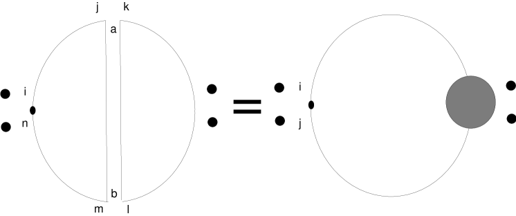
Figure 2: Bare and dressed vacuum loop calculations shown to agree to order $g^{2}$.

We calculate this bare diagram using both the ’t Hooft regularization scheme and principal value regularization and found that they are equivalent at least to order $g^{2}$:

$$\langle\bar{\psi}\psi\rangle=-N\;C_{2}(F)\;\frac{1}{\pi^{2}}\frac{g^{2}}{m}=-\frac{(N^{2}-1)}{2}\;\frac{1}{\pi^{2}}\frac{g^{2}}{m},$$ (12)

where the second Casimir constant of the fundamental representation arises from $T^{a}_{ij}T^{a}_{ji}=Tr(C_{2}(F){\mathbf{I}}_{F})=C_{2}(F)N$ after contraction over group matrix indices because of the closed fermion loop. We note that in the large $N$ limit where $g^{2}N\sim const.$, the condensate $\langle\bar{\psi}\psi\rangle\sim N$ as it should. We also note that in the large $m$ limit it goes to zero as $1/m$ in agreement with the general discussions presented in the Introduction.

The second approach to the same calculation is to take the dressed ’t Hooft propagator and expand it to the first order in $g^{2}$ (from the definition of the condensate we have to take the difference between the dressed and free propagator):

$$\int\frac{dp_{-}dp_{+}}{(2\pi)^{2}}\left[\right. \delta{ij} \;\frac{i(\gamma_{-}p_{+}+\gamma_{+}p_{-}+m)}{2p_{+}p_{-}-m^{2}+g^{2}N/\pi-g^{2}N|p_{-}|/\pi\lambda-i\epsilon}$$

$$-\delta{ij} \;\frac{i(\gamma_{-}p_{+}+\gamma_{+}p_{-}+m)}{2p_{+}p_{-}-m^{2}-i\epsilon}\left.\right].$$

For small values of g we can expand the denominator of the first term so that we have:

$$\frac{1}{2p_{+}p_{-}-m^{2}+g^{2}N/\pi-g^{2}N|p_{-}|/\pi\lambda-i\epsilon}=$$

$$\frac{1}{2p_{+}p_{-}-m^{2}-g^{2}N|p_{-}|/\pi\lambda-i\epsilon}\left[1-\frac{g^{2}N/\pi}{2p_{+}p_{-}-m^{2}-g^{2}N|p_{-}|/\pi\lambda-i\epsilon}\right].$$

The first term of the expansion cancels the bare propagator in CPV regularization where terms containing $\lambda$ are simply dropped. Therefore we have the integral:

$$\int\frac{dp_{-}dp_{+}}{(2\pi)^{2}}\;\delta{ij}\frac{g^{2}N/\pi}{[2p_{+}p_{-}-m^{2}-i\epsilon]^{2}}.$$ (14)

The result is the same as above (12) in the large $N$ limit and agrees with the large m expansion of formula (2), (see Ref.[17]). The moral of this section is that we are confident that the perturbative calculation gives the correct expression for the condensate (1) in this completely solvable example. Now we would like to apply this approach to a model which (unlike the ’t Hooft model) is not completely solvable, but is much more interesting because it includes nontrivial vacuum structure labeled by an integer number $k=0,1,...N-1$. We consider this problem in the next section.

3 Condensate with Adjoint Fermions

Now we want to do the same calculation for two dimensional QCD where we take the fermions to be in the adjoint representation. The QCD lagrangian is the same as before with the only difference that the generators of the group are the structure constants of the group

$$(T^{a})_{bc}=-if_{abc}~{}~{}~{}~{}~{}~{}~{}~{}~{}a=1,2\ldots(N^{2}-1).$$ (15)

We now repeat our previous calculation of the first diagram in Figure (2) with the following result:

$$\langle\bar{\psi}\psi\rangle=-(N^{2}-1)\;C_{2}(A)\;\frac{m}{\pi^{2}}\frac{g^{2}}{m^{2}}=-N(N^{2}-1)\;\frac{g^{2}}{\pi^{2}m},$$ (16)

where we take into account the value for the second Casimir constant for the adjoint representation:

$$T^{a}_{ij}T^{a}_{ji}=Tr(C_{2}(A){\mathbf{I}}_{A})=C_{2}(A)(N^{2}-1).$$ (17)

This result corresponds to the trivial vacuum, i.e. $k=0$. We would like to do the same perturbative calculations for a nontrivial vacuum state $|k\rangle$ as well. Recall that the case of fermions in the adjoint representation has long been known [12] to possess $N$ different vacua corresponding to fundamental external charges at the boundaries of the universe. This is equivalent to a universe with a background color electric field analagous to the $\theta$-vacua in Coleman’s analysis of the Schwinger model[21]. Different vacua in the nonabelian case have, in general, different vacuum energy and can be labeled by discrete values of $\theta$:

$$\theta_{k}=\frac{2\pi}{N}k\;\;\;k=0,1,\ldots(N-1).$$ (18)

These vacua are unstable when the dynamical fermions are in the fundamental representation because they can screen the charges at the edges of the universe to form a trivial vacuum[12]. This is the analogy of pair creation in the massive Schwinger model. When the fermions are in the adjoint representation such a screening cannot occur and therefore there is a nontrivial vacuum structure and consequently a nontrivial dependence of the observables on this vacuum angle $k$.

Now the question is: Is it possible to obtain a nontrivial dependence on the topological angle $k$ from the perturbative calculation, which apparently does not contain any information regarding the topological properties of the theory at all? Are we able to see the effect of the vacuum angle $\theta_{k}$ in a perturbative expansion $\sim\sum_{n}c_{n}(\frac{g^{2}}{m^{2}})^{n}$ or is this impossible in principle?

The answer to the question formulated above is: yes, we can extract information about vacuum topological properties of the theory. In fact, this information is contained in the coefficients $c_{n}$ of the perturbative expansion in powers of $g^{2}/m^{2}$. The point is that external charges at the boundaries of the universe cannot, of course, talk in the gauge theory to vacuum fermions directly, but they can communicate via gluons as soon as the external charges act as sources for the latter. It is therefore clear that in order to see a nontrivial $k-$dependence in the fermion condensate, $\langle\bar{\psi}\psi\rangle$, we should go beyond the leading term (16) in the expansion over $g^{2}/m^{2}$ and take into account terms of higher orders in $1/m$ which are accompanied by powers of the gluon field. Technically, this problem amounts to a calculation of the heavy fermion loop in an external gluon field (see Fig.(3)) which does depend on the topological number $k$. In our case both the use of the perturbative fermion propagator and retaining only a finite number of powers of the external field (and its derivatives) are justified by the smallness of the parameter $g^{2}/m^{2}$. This procedure results in a particular form of the Operator Product Expansion in powers of $1/m$ (known also as the heavy quark expansion). Note that by gauge invariance the expansion in external field starts from a term of second order in the field, and this is why we expect to get a nonzero effect at the level of order $g^{4}/m^{3}$.

Therefore, at large $m$ we are justified in the use of perturbation theory in order to reduce the problem of the calculation of $\langle k|\bar{\psi}\psi|k\rangle$ to the problem of the calculation of the gluon condensate $\langle k|TrG_{\mu\nu}G^{\mu\nu}|k\rangle$. The corresponding method is well-known and we refer to a nice technical review[22] of the subject. The result of the calculation is::

$$\langle k|\bar{\psi}\psi|k\rangle-\langle 0|\bar{\psi}\psi|0\rangle= - \frac{1}{12\pi}\frac{g^{2}N}{m^{3}}\left(\langle k|G_{\mu\nu}^{a}G^{a\mu\nu}|k\rangle-\langle 0|G_{\mu\nu}^{a}G^{a\mu\nu}|0\rangle\right)$$ (19)

$$+ O(1/m^{5}).$$

Figure 3: Heavy fermion loop in an external gluon field

The problem of the dependence of the gluon condensate $\langle k|G_{\mu\nu}^{a}G^{a\mu\nu}|k\rangle$ on nontrivial vacuum structure in pure gluodynamics in two dimensions has been solved earlier in [7]. The dynamical heavy quarks with mass $m$ will bring some order $1/m^{2}$ corrections to this result and we neglect these corrections at the moment (see the corresponding calculations in the next section). We quote the relevant formula for the gluon condensate in Minkowski space rather than in Euclidean space, where it was originally obtained [7]:

$$\langle k|G_{\mu\nu}^{a}G^{a\mu\nu}|k\rangle-\langle k=0|G_{\mu\nu}^{a}G^{a\mu\nu}|k=0\rangle=g^{2}\frac{2k(N-k)(N+1)}{N}.$$ (20)

Therefore, the final expression for the condensate as a function of the vacuum label $k$ takes the following form:

$$\langle k|\bar{\psi}\psi|k\rangle-\langle 0|\bar{\psi}\psi|0\rangle=-\frac{N}{6\pi}\frac{g^{4}}{m^{3}}\frac{k(N-k)(N+1)}{N}.$$ (21)

We close this section with a few remarks. First, as was expected, a nontrivial dependence on $k$ appears in the final formula only at the level $\sim g^{4}/m^{3}$ and therefore is relatively small in large $m$ limit. Nevertheless, formula (21) demonstrates that all physical properties are different for different vacua label $k$. Vacuum condensates are different. String tensions[7] are different and therefore the mass spectrum is different. Vacuum energies are also different. We demonstrated this fact by keeping only the leading $1/m$ terms. However, we believe that the statement has a more general origin and it is hard to believe that different vacua could become identical for a finite value of $m$ as long as the two parameters $m$ and $k$ are independent of each other. Our last remark regarding formula (19) is that the function which appears there has a property which was expected from the very beginning[12] - it is a periodic function such that states $|k=0\rangle$ and $|k=N\rangle$ are equivalent. Therefore, we do not obtain a new state each time we increase the label $k$. Instead, we return to the starting state after $N$ steps have been made. We notice also the symmetry property $k\Leftrightarrow(N-k)$ which was also expected[7].

4 Low Energy Theorems

The purpose of this section is twofold. First of all, the low energy theorems make it possible to investigate the behavior of vacuum condensates with changing quark mass $m$ in the vicinity of parameters where those condensates are known, i.e. at $m\rightarrow\infty$. This information might help in understanding the qualitative features of the model in general and its vacuum structure in particular. The second goal of this study is the calculation of the $\frac{1}{m^{2}}$ corrections to the gluon condensate calculated in pure gluodynamics [7] due to the presence of matter fields.

A similar study of the low energy theorems in the ’t Hooft model was carried out for the first time in ref. [14], for vanishing fermion mass, where the corresponding quark and gluon condensates have been calculated. This program was pushed forward in Ref.[17] where the previous result was generalised to arbitrary quark mass in the ’t Hooft model.

The main idea of the derivation of the low energy theorems is quite simple[23]. From the definition of the Path Integral, the variation of the gluon condensate with mass $m$ is determined by the following correlation function

$$\frac{d}{dm}\langle G^{a}_{\mu\nu}G^{a\mu\nu}\rangle=-i\lim_{q\rightarrow 0}\int d^{2}xe^{iqx}\langle 0|T\{\bar{\psi}\psi(x),G^{a}_{\mu\nu}G^{a\mu\nu}(0)\}|0\rangle.$$ (22)

At the same time, the obtained correlation function can be explicitly calculated due to the following identity

$$i\lim_{q\rightarrow 0}\int d^{2}xe^{iqx}\langle 0|T\{\bar{\psi}\psi(x),G^{a}_{\mu\nu}G^{a\mu\nu}(0)\}|0\rangle=-\frac{4}{g^{2}}\frac{d}{d(1/g^{2})}\langle\bar{\psi}\psi\rangle.$$ (23)

Up to this point the derivation in $QCD_{2}$ is identical to that in $QCD_{4}$. The only relevant point is the form of the Lagrangian (3) and not the specific properties of the theory which of course depend on the dimensionality of the space-time. The difference appears in the explicit calculation of the right hand side of Eq.(23).

In $QCD_{4}$ the corresponding calculation [23] of $\frac{d}{d(1/g^{2})}\langle\bar{\psi}\psi\rangle$ is based on the observation that due to the asymptotic freedom and to the absence of mass parameter other than $M$ (the ultraviolet cut-off), the dependence on $g$ comes exclusively through $\Lambda_{QCD}\sim M\exp{-\frac{8\pi^{2}}{bg^{2}(M)}}$ where $b=11N/3-2N_{f}/3$ is the first term in the Gell-Mann-Low $\beta$-function.

In the present case of $QCD_{2}$ the dependence on $g^{2}$ is known exactly in large $m$ limit (21). Therefore, we can explicitly calculate the behavior of the vacuum condensate $\langle G^{a}_{\mu\nu}G^{a\mu\nu}\rangle$ with variation of the quark mass $m$:

$$\frac{d}{dm}\left(\langle G^{a}_{\mu\nu}G^{a\mu\nu}\rangle_{k}-\langle G^{a}_{\mu\nu}G^{a\mu\nu}\rangle_{0}\right)=\frac{N}{\pi}\frac{4g^{4}}{3m^{3}}\frac{k(N-k)(N+1)}{N}.$$ (24)

Note that in this formula we keep only the information relevant to the $k$-vacuum dependence. As mentioned above, there is a leading term ($\sim g^{2}/m$) in the fermion condensate (16) which does not contain any $k-$dependence. A similar term in the gluon condensate depends on subtraction and normalization procedures but we will not discuss this issue here. However, the difference in condensates between two vacuum states has an absolute meaning and the corresponding expression is given by eq. (24).

Formula (24) makes it possible to calculate the finite correction due to the dynamical heavy quark to the gluon condensate calculated previously [7] in pure gluodynamics. Integrating Eq.(24) at large $m$, we obtain

$$\langle k|G_{\mu\nu}^{a}G^{a\mu\nu}|k\rangle-\langle 0|G_{\mu\nu}^{a}G^{a\mu\nu}|0\rangle=g^{2}\frac{2k(N-k)(N+1)}{N}(1-\frac{1}{3}\frac{g^{2}N}{\pi m^{2}}).$$ (25)

The correction $\sim\frac{g^{2}N}{\pi m^{2}}$ in this formula is not suppressed in the large $N$ limit. This is in accordance with the general expectation that fluctuations of adjoint matter fields (unlike fundamental matter) are not suppressed by a factor $1/N$.

One can go a little bit further in the analysis of the low energy theorems by taking advantage of the specific property of two dimensional $QCD$ that the only dimensionless combination in the theory is $g^{2}/m^{2}$. Therefore, without loss of generality one can present the fermion condensate in the following form:

$$\langle\bar{\psi}\psi\rangle=mf(\frac{g^{2}}{m^{2}}),$$ (26)

with some function $f(x=\frac{g^{2}}{m^{2}})$. In this case the derivative with respect to $m$ and derivative with respect to $g$ are related to each other. At the same time, as we observed earlier, the derivative $\frac{d}{d(1/g^{2})}\langle\bar{\psi}\psi\rangle$ is reduced to some correlation function (23) which describes the dependence of the gluon condensate on $m$ (22). Therefore one can relate the gluon and quark condensate exactly without any approximations using only very general properties of the theory. Indeed, from identities

$$\frac{d}{dm}\left(\frac{\langle\bar{\psi}\psi\rangle}{m}\right)=-2\frac{g^{2}}{m^{3}}f^{\prime}(x),$$

$$\frac{d}{d(1/g^{2})}\langle\bar{\psi}\psi\rangle=-\frac{g^{4}}{m}f^{\prime}(x),$$ (27)

one obtains:

$$\frac{d}{d(1/g^{2})}\langle\bar{\psi}\psi\rangle=\frac{g^{2}m^{2}}{2}\frac{d}{dm}\left(\frac{\langle\bar{\psi}\psi\rangle}{m}\right).$$ (28)

Now combining the low energy theorems (22,23) with (28) we obtain the exact relation between quark and gluon condensates:

$$\frac{1}{2}\frac{d}{dm}\langle G_{\mu\nu}^{a}G^{a\mu\nu}\rangle=m^{2}\frac{d}{dm}\left(\frac{\langle\bar{\psi}\psi\rangle}{m}\right).$$ (29)

This relation was derived earlier in [17] using a different approach. One can rederive our previous formula for the gluon condensate (25) using the exact relation (29) and the expression (21) for the quark condensate in the asymptotic region.

An exact relation between quark and gluon condensates should not be considered as a big surprise. Such a relation is a direct consequence of the fact that in two dimensional $QCD$ the gluons are not dynamical degrees of freedom.

5 Conclusion

The main results of this paper are given by Eqs.(21),(25). We explicitly calculated the quark and gluon condensates in $QCD_{2}(N)$ coupled to adjoint matter as a function of the nontrivial vacuum label $k$. Our formulae are valid only in the vicinity of large $m$, but the obtained results suggest that all observables do depend on the specific vacuum state in which we live.

In principle, one can further generalize formula (19) in order to include higher dimensional gluon condensates. One can derive the next term in the expansion:

$$\langle\bar{\psi}\psi\rangle = -\frac{g^{2}}{\pi^{2}m}Tr\left[T(R)T(R)\right]-\frac{1}{12\pi}\frac{g^{2}}{m^{3}}\langle Tr\left[G^{\mu\nu}G_{a\mu\nu}\right]\rangle$$

$$- \frac{1}{12\pi}\frac{g^{2}}{m^{5}}\left(\langle Tr\left[(D_{\alpha}G^{\mu\nu})(D^{\alpha}G_{\mu\nu})\right]\rangle+\frac{1}{2}\langle Tr\left[G_{\mu\nu}D^{2}G^{\mu\nu}\right]\rangle\right.$$

$$- \left.\frac{1}{3}\langle Tr\left[(D_{\alpha}G^{\alpha\mu})(D^{\beta}G_{\beta\mu})\right]\rangle\right)+\ldots~{}~{},$$

where $T(R)$ are the generators in the representation R of SU(N). Note that Eq.(5) is valid for arbitrary representation of SU(N). Unfortunately, we do not know the higher dimensional condensates which appear in (5). The only thing we know for sure is the fact that the $k$-dependence of each condensate should be a periodic function similar to, but not necessarily the same as, (21). One can reverse this argument. If we knew the fermion condensate in $QCD_{2}^{adjoint}$ for arbitrary $m$ exactly, (similar to Eq.(2) in the ’t Hooft model), we would be able to calculate all high dimensional gluon condensates as a function of $k$. This problem is probably too complicated and equivalent to the complete solution of $QCD_{2}^{adjoint}$ which presently is not available.

We conclude this paper with the following project for future investigation. One may try to use our results with heavy quark mass to generalize the string picture originally derived in [24] for the pure gauge 2D theory without dynamical degrees of freedom. By introducing a heavy quark we have essentially introduced the physical degrees of freedom without noticeably changing the internal gluodynamics. Therefore, we expect that the introduction of the heavy quark might be the first step in the direction of a string description of dynamical degrees of freedom. We probably need to implement some dynamics on the string-sheet boundary which would correspond to a heavy, but dynamical, quark.

6 Acknowledgements

This work was supported in part by the Natural Sciences and Engineering Research Council of Canada.

References

-
[1]
G. Bhanot, K. Demeterfi and I.R. Klebanov,
Phys. Rev.
D48, 4980, (1993),
D. Kutasov, Nucl. Phys. B414, 33, (1994) . - [2] A. Smilga, Phys.Rev. D. 49, 6836 (1994).
- [3] F. Lenz, M. Shifman and M. Thies, Phys.Rev. D51, 7060 (1995)
- [4] I. Kogan and A. Zhitnitsky, Nucl.Phys. B465, 99 (1996)
-
[5]
D.J. Gross, A.V. Smilga, A. Matytsin and I.R. Klebanov,
Nucl. Phys. B461, 109, (1996) hep-th/9511104;
E. Abdalla, R. Mohayaee and A. Zadra, hep-th/9604063 -
[6]
G. Semenoff, K. Zarembo Nucl.Phys.
B480, 317 (1996)
C.R. Gattringer, L. Paniak and G. Semenoff hep-th/9612030. -
[7]
L. Paniak, G. Semenoff and A. Zhitnitsky,
Nucl.Phys. B487, 191 (1997),
L. Paniak, G. Semenoff and A. Zhitnitsky, hep-th/9701270 (1997). - [8] S. Pinsky and R. Mohr hep-th/9610007 (1996)
- [9] G. McCartor, D. Robertson and S. Pinsky, hep-th/9612083, to appear in Phys. Rev.D
- [10] G. McCartor, hep-th/9609140, to appear in Int. J. Mod.Phys. A
- [11] H.R. Christiansen, hep-th/9704020.
- [12] E. Witten, Nuov.Cim. 51A, 325 (1979)
- [13] G. ’t Hooft, Nucl.Phys. B75, 461 (1974).
- [14] A. Zhitnitsky Phys.Lett. 165 405 (1985); Sov.J.Nucl.Phys. 43, 999 (1986):ibid. Sov.J.Nucl.Phys. 44, 139 (1986)
- [15] M. Li Phys.Rev. D34, 3888 (1986)
- [16] F. Lenz et al, Ann. Phys. 208, 1, (1991).
- [17] M. Burkardt, Phys.Rev. D53, 933, (1996)
- [18] S.L. Adler and R. Dashen, Current Algebras and Applications to particle Physics, Benjamin, New York, 1968.
- [19] C. Callan, N. Coote and D. Gross, Phys.Rev. D13, (1976)
- [20] M. Einhorn, Phys.Rev. D14, 3451 (1976)
- [21] S. Coleman, Ann.Phys. 101, 239 (1976)
- [22] V. Novikov et al., Fortschritte Phys. 32, 585 (1984).
- [23] V. Novikov et al., Nucl.Phys. B191, 301 (1981).
- [24] D. J. Gross and W.Taylor, Nucl. Phys. B400, 181, (1993), Nucl. Phys. B403, 395, (1993).