Limits on Anomalous Top Couplings from $Z$ Pole Physics

Abstract

We obtain constraints on possible anomalous interactions of the top quark with the electroweak vector bosons arising from the precision measurements at the $Z$ pole. In the framework of $SU(2)_{L}\otimes U(1)_{Y}$ chiral Lagrangians, we examine all effective CP–conserving operators of dimension five which induce fermionic currents involving the top quark. We constrain the magnitudes of these anomalous interactions by evaluating their one–loop contributions to the $Z$ pole physics. Our analysis shows that the operators that contribute to the LEP observables get bounds close to the theoretical expectation for their anomalous couplings. We also show that those which break the $SU(2)_{C}$ custodial symmetry are more strongly bounded.

I Introduction

The Standard Model (SM) of electroweak interactions has passed through an intense experimental scrutiny that confirmed several of its predictions. In particular, the precise LEPI measurements performed at the $Z$ pole show that the SM describes extremely well the couplings between the gauge bosons and the light fermions [1]. Notwithstanding, the couplings of the top quark to the gauge bosons are still rather poorly measured at the Tevatron $p\bar{p}$ collider [2]. Furthermore, some other elements of the SM, such as the symmetry breaking mechanism, have not been directly tested yet.

If the breaking of the $SU(2)_{L}\otimes U(1)_{Y}$ symmetry takes place via the Higgs mechanism with a relatively light elementary Higgs boson, both the symmetry breaking and the fermion mass generation can have a common origin. However, if no fundamental Higgs particle is present in the theory, the mechanism that breaks the electroweak symmetry and the one that gives rise to the fermion masses are not necessarily related, and we can envisage a breaking in the universality of the fermionic interactions [3]. One may expect that the top quark, being the heaviest of the known fermions, should be more sensitive to the existence of new physics in the electroweak breaking sector. This is certainly the case if, for instance, the breaking of the electroweak symmetry occurs dynamically via the appearance of a $t\bar{t}$ condensate [4].

Whatever the dynamics of the symmetry breaking mechanism is, renormalizability requires that this breaking must occur spontaneously. This leads to the existence of Goldstone bosons associated with the broken directions which become the longitudinal components of the massive gauge bosons. Assuming this as our starting point, we can build effective low–energy Lagrangians which describe the interactions of these Goldstone bosons. The self–interactions of the Goldstone bosons, to lowest order, are totally determined by the symmetry breaking pattern and it is described in terms of a unique dimensionful parameter $v$. However, the interactions between the Goldstone bosons and other fields, such as fermions, involve new unknown parameters that, when the interaction is gauged, leads, in general, to universality violation in the couplings between gauge boson and fermions.

Limits on universality violation in the interactions of the top quark to the gauge bosons have been studied before in Ref. [3, 5] where the authors included only dimension–four operators. In this work, we study the most general CP invariant dimension–five Lagrangian for the interactions between the Goldstone bosons and the top and bottom quarks. In the unitary gauge, these Lagrangians give rise to non–universal couplings of the top and bottom quarks to the gauge bosons. Since the SLC and LEPI achieved a precision of the order of $0.1$ percent in some observables, the $Z$ pole physics is the best available source of information on these interactions. We obtain the constraints on these anomalous top couplings by imposing that their one–loop contributions to the electroweak parameters are compatible with the $Z$ pole data [6].

II Effective Lagrangians

If the Higgs boson, responsible for the electroweak symmetry breaking, is very heavy, it can be effectively removed from the physical low–energy spectrum. In this case and for dynamical symmetry breaking scenarios relying on new strong interactions, one is led to consider the most general effective Lagrangian which employs a nonlinear representation of the spontaneously broken $SU(2)_{L}\otimes U(1)_{Y}$ gauge symmetry [7]. The resulting chiral Lagrangian is a non–renormalizable nonlinear $\sigma$–model coupled in a gauge–invariant way to the Yang-Mills theory. This model independent approach incorporates by construction the low–energy theorems [8], that predict the general behavior of Goldstone boson amplitudes, irrespective of the details of the symmetry breaking mechanism. Unitarity requires that this low–energy effective theory should be valid up to some energy scale smaller than $4\pi v\simeq 3$ TeV, where new physics would come into play.

In order to specify the effective Lagrangian for the Goldstone bosons, we assume that the symmetry breaking pattern is $G=SU(2)_{L}\otimes U(1)_{Y}$ $\longrightarrow$ $H=U(1)_{\text{em}}$, leading to just three Goldstone bosons $\pi^{a}$ ($a=1,2,3$). With this choice, the building block of the chiral Lagrangian is the dimensionless unimodular matrix field $\Sigma$,

$$\Sigma=\exp\left(i\frac{\pi^{a}\tau^{a}}{v}\right)\;,$$ (1)

where $\tau^{a}$ ($a=1,2,3$) are the Pauli matrices. We implement the $SU(2)_{C}$ custodial symmetry by imposing a unique dimensionful parameter, $v$, for charged and neutral fields. Under the action of $G$ the transformation of $\Sigma$ is

$$\Sigma\rightarrow\Sigma^{\prime}=L~{}\Sigma~{}R^{\dagger}\;,$$

with $L=\exp\left(i\frac{\alpha^{a}\tau^{a}}{2}\right)$ and $R=\exp\left(iy\frac{\tau^{3}}{2}\right)\;$. $\alpha^{a}$ and $y$ are the parameters of the transformation.

The gauge fields are represented by the matrices $\hat{W}_{\mu}=\tau^{a}W^{a}_{\mu}/(2i)$, $\hat{B}_{\mu}=\tau^{3}B_{\mu}/(2i)$, while the associated field strengths are given by

$$\begin{array}[]{ll}\hat{W}_{\mu\nu}=&\partial_{\mu}\hat{W}_{\nu}-\partial_{\nu}\hat{W}_{\mu}-g\left[\hat{W}_{\mu},\hat{W}_{\nu}\right]\;,\\ \hat{B}_{\mu\nu}=&\partial_{\mu}\hat{B}_{\nu}-\partial_{\nu}\hat{B}_{\mu}\;.\end{array}$$ (2)

In the nonlinear representation of the gauge group $SU(2)_{L}\otimes U(1)_{Y}$, the mass term for the vector bosons is given by the lowest order operator involving the matrix $\Sigma$. Therefore, the kinetic Lagrangian for the gauge bosons reads

$${\cal L}_{B}=\frac{1}{2}{\rm Tr}\left(\hat{W}_{\mu\nu}\hat{W}^{\mu\nu}+\hat{B}_{\mu\nu}\hat{B}^{\mu\nu}\right)+\frac{v^{2}}{4}{\rm Tr}\left(D_{\mu}\Sigma^{\dagger}D^{\mu}\Sigma\right)\;,$$ (3)

where the covariant derivative of the field $\Sigma$ is $D_{\mu}\Sigma=\partial_{\mu}\Sigma-g\hat{W}_{\mu}\Sigma+g^{\prime}\Sigma\hat{B}_{\mu}$.

In order to include fermions in this framework, we must define their transformation under $G$. Following Ref. [3], we postulate that matter fields feel directly only the electromagnetic interaction $f\rightarrow f^{\prime}=e^{iyQ_{f}}\;f$, where $Q_{f}$ stands for the electric charge of fermion $f$. The usual fermion doublets are then defined with the following transformation under $G$

$$\Psi_{L}=\Sigma\left(\begin{array}[]{c}f_{1}\\[-2.84544pt] f_{2}\end{array}\right)_{L}\;\rightarrow\Psi^{\prime}_{L}=L~{}\exp(iyY/2)\Psi_{L},$$ (4)

where $Q_{f_{1}}-Q_{f_{2}}=1$ and with $Y=2Q_{f_{1}}-1$. Right–handed fermions are just the singlets $f_{R}$. In this framework, the lowest–order interactions between fermions and vector bosons that can be built are of dimension four, leading to anomalous vector and axial–vector couplings, which were analyzed in detail in Ref. [5].

In order to construct the most general Lagrangian describing these interactions, it is convenient to define the vector and tensor fields

$$\begin{array}[]{l}\Sigma_{\mu}^{a}=-\frac{\displaystyle i}{\displaystyle 2}{\rm Tr}\left(\tau^{a}V_{\mu}^{R}\right)~{}=~{}-\frac{\displaystyle i}{\displaystyle 2}{\rm Tr}\left(\tau^{a}\Sigma^{\dagger}D_{\mu}\Sigma\right)\;,\\ \Sigma_{\mu\nu}^{a}=-i\;{\rm Tr}\left[\tau^{a}\Sigma^{\dagger}\left[D_{\mu},D_{\nu}\right]\Sigma\right]\;.\end{array}$$ (5)

Under $G$, $\Sigma_{\mu}^{3}$ and $\Sigma_{\mu\nu}^{3}$ are invariant while $\Sigma_{\mu(\mu\nu)}^{\pm}\rightarrow{\Sigma^{\prime}}_{\mu(\mu\nu)}^{\pm}=e^{\pm iy}\Sigma_{\mu(\mu\nu)}^{\pm}$, where $\Sigma_{\mu(\mu\nu)}^{\pm}=(1/\sqrt{2})(\Sigma_{\mu(\mu\nu)}^{1}\mp i\Sigma_{\mu(\mu\nu)}^{2})$.

The basic fermionic elements for the construction of neutral- and charged-current effective interactions are

$$\begin{array}[]{ll}\Delta_{X}(q,q^{\prime})\equiv\bar{q}P_{X}q^{\prime}\;,&\Delta^{\mu}_{X}(q,q^{\prime})\equiv\bar{q}P_{X}\tilde{D}^{\mu}q^{\prime}\;,\\ \overline{\Delta^{\mu}_{X}}(q,q^{\prime})\equiv\overline{\tilde{D}^{\mu}q}P_{X}q^{\prime}\;,&\Delta^{\mu\nu}_{X}(q,q^{\prime})\equiv\bar{q}\sigma^{\mu\nu}P_{X}q^{\prime}\;,\end{array}$$ (6)

where $P_{X}$ ($X=0$, $5$, $L$, and $R$) stands for $I$, $\gamma^{5}$, $P_{L}$, and $P_{R}$ respectively, with $I$ being the identity matrix and $P_{L(R)}$ the left (right) chiral projector. The fermionic field $q$ ($q^{\prime}$) represents any quark flavor. $\tilde{D}^{\mu}$ represents the electromagnetic covariant derivative.

The most general neutral–current interactions of dimension–five, which are invariant under nonlinear transformations under $G$, are [9]:

$$\begin{array}[]{ll}{\cal L}^{\text{NC}}=&a_{1}^{\text{NC}}~{}\Delta_{0}(t,t)~{}\Sigma_{\mu}^{+}\Sigma^{-\mu}+a_{2}^{\text{NC}}~{}\Delta_{0}(t,t)~{}\Sigma_{\mu}^{3}\Sigma^{3\mu}+i~{}a_{3}^{\text{NC}}~{}\Delta_{5}(t,t)~{}\partial^{\mu}\Sigma^{3}_{\mu}\\ &+i~{}b_{1}^{\text{NC}}~{}\Delta^{\mu\nu}_{0}(t,t)~{}\mbox{Tr}\left[T\hat{W}_{\mu\nu}\right]+b_{2}^{\text{NC}}~{}\Delta^{\mu\nu}_{0}(t,t)~{}B_{\mu\nu}\\ &+i~{}b_{3}^{\text{NC}}~{}\Delta^{\mu\nu}_{0}(t,t)~{}\left(\Sigma^{+}_{\mu}\Sigma^{-}_{\nu}-\Sigma^{+}_{\nu}\Sigma^{-}_{\mu}\right)~{}+i~{}c_{1}^{\text{NC}}~{}\left(\Delta^{\mu}_{0}(t,t)-\overline{\Delta^{\mu}_{0}}(t,t)\right)\Sigma^{3\mu}\;,\end{array}$$ (7)

and the charged–current interactions are

$$\begin{array}[]{ll}{\cal L}^{\text{C}C}=&a_{1L}^{\text{CC}}~{}\Delta_{L}(t,b)~{}\Sigma_{\mu}^{+}\Sigma^{3\mu}+a_{1R}^{\text{CC}}~{}\Delta_{R}(t,t)~{}\Sigma_{\mu}^{+}\Sigma^{3\mu}\\ &+ia_{2L}^{\text{CC}}~{}\Delta_{L}(t,b)~{}\tilde{D}^{\mu}\Sigma_{\mu}^{+}+ia_{2R}^{\text{CC}}~{}\Delta_{R}(t,t)~{}\tilde{D}^{\mu}\Sigma_{\mu}^{+}\\ &+\,b_{1L}^{\text{CC}}\Delta^{\mu\nu}_{L}(t,b)~{}\Sigma_{\mu\nu}^{+}+\,b_{1R}^{\text{CC}}~{}\Delta^{\mu\nu}_{R}(t,b)~{}\Sigma_{\mu\nu}^{+}\\ &+\,b_{2L}^{\text{CC}}~{}\Delta^{\mu\nu}_{L}(t,b)~{}\left(\Sigma^{+}_{\mu}\Sigma^{3}_{\nu}-\Sigma^{+}_{\nu}\Sigma^{3}_{\mu}\right)+\,b_{2R}^{\text{CC}}~{}\Delta^{\mu\nu}_{R}(t,b)~{}\left(\Sigma^{+}_{\mu}\Sigma^{3}_{\nu}-\Sigma^{+}_{\nu}\Sigma^{3}_{\mu}\right)\\ &+i~{}c_{1L}^{\text{CC}}~{}\Delta^{\mu}_{L}(t,b)\Sigma^{+}_{\mu}+i~{}c_{1R}^{\text{CC}}~{}\Delta^{\mu}_{R}(t,b)\Sigma^{+}_{\mu}~{}+~{}\mbox{h.c.}\;.\end{array}$$ (8)

In the unitary gauge, we can rewrite these interactions as a scalar (${\cal L}_{S}$), a vector (${\cal L}_{V}$), and a tensorial (${\cal L}_{T}$) Lagrangian involving the physical fields.

$$\begin{array}[]{ll}{\cal L}_{S}=&\frac{\displaystyle g^{2}}{\displaystyle 4\Lambda}\Biggl{[}\bar{t}t\Bigl{(}2\alpha_{1}^{NC}W^{+}_{\mu}W^{-\mu}+\frac{\alpha_{2}^{NC}}{c_{W}^{2}}Z^{\mu}Z_{\mu}\Bigr{)}\Biggr{]}+i\frac{\displaystyle g}{\displaystyle 2c_{W}\Lambda}\alpha_{3}^{NC}\bar{t}\gamma^{5}t\partial^{\mu}Z_{\mu}\\ &+\frac{\displaystyle g^{2}}{\displaystyle 2\sqrt{2}\Lambda c_{W}}\Biggl{\{}\bar{t}~{}\Bigl{[}\alpha_{1L}^{CC}(1-\gamma^{5})+\alpha_{1R}^{CC}(1+\gamma^{5})\Bigr{]}b\;W_{\mu}^{+}Z^{\mu}\\ &+\bar{b}\Bigl{[}\alpha_{1L}^{CC}(1+\gamma^{5})+\alpha_{1R}^{CC}(1-\gamma^{5})\Bigr{]}t\;W^{-}_{\mu}Z^{\mu}\Biggr{\}}\\ &+i\frac{\displaystyle g}{\displaystyle 2\sqrt{2}\Lambda}\Biggl{\{}\bar{t}~{}\Bigl{[}\alpha_{2L}^{CC}(1-\gamma^{5})+\alpha_{2R}^{CC}(1+\gamma^{5})\Bigr{]}b\;\left(\partial^{\mu}W_{\mu}^{+}+ieA^{\mu}W_{\mu}^{+}\right)\\ &-\bar{b}~{}\Bigl{[}\alpha_{2L}^{CC}(1+\gamma^{5})+\alpha_{2R}^{CC}(1-\gamma^{5})\Bigr{]}t\;\left(\partial^{\mu}W_{\mu}^{-}-ieA^{\mu}W_{\mu}^{-}\right)\Biggr{\}}\\ \end{array}$$ (9)

$$\begin{array}[]{ll}{\cal L}_{V}=&i~{}\frac{\displaystyle g}{\displaystyle 2c_{W}}~{}\gamma^{NC}~{}\bar{t}~{}(\tilde{D}_{\mu}t)~{}Z^{\mu}-i~{}\frac{\displaystyle g}{\displaystyle 2c_{W}}~{}\gamma^{NC}\overline{(\tilde{D}_{\mu}t)}~{}t~{}Z^{\mu}\\ &+i~{}\frac{\displaystyle g}{\displaystyle 2\sqrt{2}}~{}\bar{t}\left[\gamma_{L}^{CC}(1-\gamma^{5})+\gamma_{R}^{CC}(1+\gamma^{5})\right]~{}(\tilde{D}_{\mu}b)~{}W{+^{\mu}}\\ &-i~{}\frac{\displaystyle g}{\displaystyle 4c_{W}}~{}\overline{(\tilde{D}_{\mu}b)}\left[\gamma_{L}^{CC}(1+\gamma^{5})+\gamma_{R}^{CC}(1-\gamma^{5})\right]~{}t~{}W^{-\mu}\end{array}$$ (10)

$$\begin{array}[]{ll}{\cal L}_{T}=&\frac{\displaystyle 1}{\displaystyle 4\Lambda}\Biggl{[}\bar{t}\sigma^{\mu\nu}t\;\Bigl{(}\beta_{1}^{NC}eF_{\mu\nu}+\beta_{2}^{NC}\frac{g}{c_{W}}Z_{\mu\nu}+4ig^{2}\beta_{3}^{NC}W_{\mu}^{+}W_{\nu}^{-}\Bigr{)}\Biggr{]}\\ &+\frac{\displaystyle g}{\displaystyle 2\sqrt{2}\Lambda}\Biggl{\{}\bar{t}\;\sigma^{\mu\nu}\;\Bigl{[}\beta_{L1}^{CC}(1-\gamma^{5})+\beta_{R1}^{CC}(1+\gamma^{5})\Bigr{]}b\;\Bigl{[}W^{+}_{\mu\nu}+ie\left(A_{\mu}W_{\nu}^{+}-A_{\nu}W_{\mu}^{+}\right)\Bigr{]}\\ &+\bar{b}\;\sigma^{\mu\nu}\;\Bigl{[}\beta_{L1}^{CC}(1+\gamma^{5})+\beta_{R1}^{CC}(1-\gamma^{5})\Bigr{]}t\;\Bigl{[}W^{-}_{\mu\nu}-ie\left(A_{\mu}W^{-}_{\nu}-A_{\nu}W^{-}_{\mu}\right)\Bigr{]}\\ &+i\frac{\displaystyle g}{\displaystyle c_{W}}~{}\bar{t}\;\sigma^{\mu\nu}\;\Bigl{[}\beta_{L2}^{CC}(1-\gamma^{5})+\beta_{R2}^{CC}(1+\gamma^{5})\Bigr{]}b\;\left(Z_{\mu}W_{\nu}^{+}-Z_{\nu}W_{\mu}^{+}\right)\\ &-i\frac{\displaystyle g}{\displaystyle c_{W}}~{}\bar{b}\;\sigma^{\mu\nu}\;\Bigl{[}\beta_{L2}^{CC}(1+\gamma^{5})+\beta_{R2}^{CC}(1-\gamma^{5})\Bigr{]}t\;\left(Z_{\mu}W^{-}_{\nu}-Z_{\nu}W^{-}_{\mu}\right)\;\Biggr{\}}\\ \end{array}$$ (11)

The couplings constants $\alpha$’s, $\beta$’s and $\gamma$’s are linear combinations of the $a$’s, $b$’s and $c$’s in Eqs. (7) to (8). In writing the interactions (9) and (11), the coupling constants were defined in such a way that we have a factor $g/(2c_{W})$ per $Z$ boson, $g/\sqrt{2}$ per $W^{\pm}$, and $e$ per photon. $s_{W}$ ($c_{W}$) is the sine (cosine) of the weak mixing angle, $\theta_{W}$. Similar interactions were obtained in Ref. [9], and for a linearly realized symmetry group, in Ref. [10].

In general, since chiral Lagrangians are related to strongly interacting theories, it is hard to make firm statements about the expected order of magnitude of the couplings. Notwithstanding, requiring the loop corrections to the effective operators to be of the same order of the operators themselves suggests that these coefficients are of ${\cal O}(1)$ [11]. Moreover, if the high energy theory respects chiral symmetry, we can also foresee a further suppression factor proportional to $m_{\text{top}}/\Lambda$.

As an example of the above anomalous couplings, we show their couplings for the SM with a heavy Higgs boson integrated out. In this case, we can perform the matching between the full theory and the effective Lagrangian [12]. Setting $m_{b}=0$ and keeping only the leading terms of the order $m_{\text{top}}\log(M_{H}^{2})$, we find that only two effective operators are generated

$$\alpha_{1}^{NC}=\alpha_{2}^{NC}=\frac{g^{2}m_{\text{top}}\Lambda}{16\pi^{2}M_{W}^{2}}\,\log\frac{M_{H}^{2}}{m^{2}_{\text{top}}}\;.$$ (12)

III Limits from $Z$ Pole Physics

At the one-loop level, the effective interactions (9) to (11) contribute to the $Z$ physics through universal corrections to the gauge boson propagators and non–universal ones to the $Zb\bar{b}$ vertex. The oblique anomalous corrections can be efficiently summarized in terms of the parameters $\epsilon^{1}_{\text{new}}$, $\epsilon^{2}_{\text{new}}$, and $\epsilon^{3}_{\text{new}}$ [13], whose expressions as functions of the unrenormalized gauge boson self-energies in the on–mass–shell renormalization scheme are

$$\epsilon^{1}_{\text{new}} = \frac{\Sigma_{\text{new}}^{ZZ}(M_{Z}^{2})}{M_{Z}^{2}}-\frac{\Sigma_{\text{new}}^{WW}(0)}{M_{W}^{2}}+2\;\frac{s_{W}}{c_{W}}\;\frac{\Sigma_{\text{new}}^{AZ}(0)}{M_{Z}^{2}}-\Sigma_{\text{new}}^{\;\prime\;ZZ}(M_{Z}^{2})\;,$$

$$\epsilon^{2}_{\text{new}} = \frac{\Sigma_{\text{new}}^{WW}(M_{W}^{2})-\Sigma_{\text{new}}^{WW}(0)}{M_{W}^{2}}-s_{W}^{2}\;\frac{\Sigma_{\text{new}}^{AA}(M_{Z}^{2})}{M_{Z}^{2}}$$

$$\;-2s_{W}c_{W}\left[\frac{\Sigma_{\text{new}}^{AZ}(M_{Z}^{2})-\Sigma_{\text{new}}^{AZ}(0)}{M_{Z}^{2}}\right]-c_{W}^{2}\;\Sigma_{\text{new}}^{\;\prime\;ZZ}(M_{Z}^{2})\;,$$

$$\epsilon^{3}_{\text{new}} = c_{W}^{2}\;\frac{\Sigma_{\text{new}}^{AA}(M_{Z}^{2})}{M_{Z}^{2}}+(c_{W}^{2}-s_{W}^{2})\;\frac{c_{W}}{s_{W}}\;\left[\frac{\Sigma_{\text{new}}^{AZ}(M_{Z}^{2})-\Sigma_{\text{new}}^{AZ}(0)}{M_{Z}^{2}}\right]-c_{W}^{2}\;\Sigma_{\text{new}}^{\;\prime\;ZZ}(M_{Z}^{2})\;,$$

where $\Sigma_{\text{new}}^{V_{1}V_{2}}$ is the new physics contribution to the transverse part of $V_{1}-V_{2}$ vacuum polarization, and $\Sigma_{\text{new}}^{\;\prime}\equiv d\Sigma_{\text{new}}/dq^{2}$. The above expressions are valid for an arbitrary momentum dependence of the vacuum polarization diagrams.

We parametrize the anomalous non–universal contributions to the vertex $Zb\bar{b}$ as

$$i\frac{e}{2s_{W}c_{W}}\left(\gamma_{\mu}F_{V}^{Zb}-\gamma_{\mu}\gamma_{5}F_{A}^{Zb}\right)\;.$$ (13)

Our results show that the new operators lead to pure left-handed contributions to this vertex, i.e. $F_{V}^{Zb}=F_{A}^{Zb}$, in the limit of vanishing bottom quark mass. These corrections can be cast in terms of the $\epsilon_{b}$ parameter [13, 14]

$$\epsilon^{b}_{\text{new}}=-2~{}F_{V}^{Zb}\;.$$ (14)

Recent global analyses of the LEP, SLD, and low-energy data yield the following values for the oblique parameters [6], which include the standard model and new physics contributions, i.e. $\epsilon^{i}\equiv\epsilon^{i}_{\text{S}M}+\epsilon^{i}_{\text{new}}$ ($i=1,2,3,b$)

$$\begin{array}[]{ll}\epsilon^{1}~{}=~{}(4.28\pm 1.25)\times 10^{-3}\;\;,&\;\;\;\;\;\;\;\;\epsilon^{2}~{}=~{}(-7.85\pm 2.2)\times 10^{-3}\;\;,\\ \epsilon^{3}~{}=~{}(4.13\pm 1.37)\times 10^{-3}\;\;,&\;\;\;\;\;\;\;\;\epsilon^{b}~{}=~{}(-4.45\pm 3.)\times 10^{-3}\;.\end{array}$$ (15)

In order to include low-energy observables in the extraction of the values for the $\epsilon$’s, one must assume that the vacuum polarization corrections differ from the SM ones only by terms up to order $q^{2}$ in the momentum expansion. Since this is the case for the couplings we are considering, we are allowed to use the values in Eq. (15) in our analysis. The extraction of the values of the $\epsilon$ parameters due to new physics requires the subtraction the SM contribution, which depends upon the SM parameters, and in particular, on the top quark mass $m_{\text{top}}$.

Our procedure to obtain the bounds on the operators (9) to (11) is the following: first we evaluate their corrections to the gauge boson self–energies and to the $Zb\bar{b}$ vertex using dimensional regularization [15], and neglecting the external fermion masses. Then, we use the leading non–analytic contributions from the loop diagrams to constrain the new interactions — that is, we keep only the logarithmic terms, dropping all the others. The contributions that are relevant for our analysis are easily obtained by the substitution

$\displaystyle\frac{2}{4-d}\rightarrow{\rm{log}}\;\frac{\Lambda^{2}}{\mu^{2}}\;,$

where $\Lambda$ is the energy scale which characterizes the appearance of new physics, and $\mu$ is the scale in the process, which we take to be $\mu=m_{\text{top}}$.

The contributions to the oblique parameters due to the top anomalous interactions are

$$\begin{array}[]{ll}\epsilon^{1}_{\text{new}}=&\frac{\displaystyle g^{2}}{\displaystyle 96\pi^{2}}~{}\frac{\displaystyle m^{3}_{\text{top}}}{\displaystyle\Lambda~{}M_{W}^{2}}~{}N_{c}~{}\left[12\left(\alpha_{2}^{NC}-\alpha_{1}^{NC}\right)+(12-32s_{W}^{2})\gamma^{NC}-3\gamma_{L}^{CC}\right]\log\frac{\displaystyle\Lambda^{2}}{\displaystyle\mu^{2}}\;,\\ \epsilon^{2}_{\text{new}}=&\frac{\displaystyle g^{2}}{\displaystyle 96\pi^{2}}~{}\frac{\displaystyle m_{\text{top}}}{\displaystyle\Lambda}~{}N_{c}\left[6\left(2\beta_{L1}^{CC}-\beta_{2}^{NC}-\beta_{1}^{NC}s_{W}^{2}\right)+2\gamma_{L}^{NC}-\gamma_{L}^{CC}\right]\log\frac{\displaystyle\Lambda^{2}}{\displaystyle\mu^{2}}\;,\\ \epsilon^{3}_{\text{new}}=&\frac{\displaystyle g^{2}}{\displaystyle 288\pi^{2}}~{}\frac{\displaystyle m_{\text{top}}}{\displaystyle\Lambda}~{}N_{c}~{}\left[3\left(3~{}\beta_{1}^{NC}+2~{}\beta_{2}^{NC}+2~{}\beta_{1}^{NC}s_{W}^{2}\right)~{}-2\gamma^{NC}\right]\log\frac{\displaystyle\Lambda^{2}}{\displaystyle\mu^{2}}\;,\end{array}$$ (16)

where $N_{c}=3$ is the number of colors.

The anomalous contributions to the $Zb\bar{b}$ vertex are left-handed for $m_{b}=0$, and their expression in terms of the $\epsilon_{b}$ parameter is

$$\begin{array}[]{ll}\epsilon^{b}_{\text{new}}=&\frac{\displaystyle g^{2}}{\displaystyle 32\pi^{2}}~{}\frac{\displaystyle m_{\text{top}}^{3}}{\displaystyle\Lambda M_{W}^{2}}\Biggl{\{}\left(1-3X_{W}\right)\left(\alpha_{1L}^{CC}+6~{}\beta_{L2}^{CC}-6~{}\beta_{L1}^{CC}c_{W}^{2}\right)\\ &+~{}\alpha_{2L}^{CC}\left[1+c_{W}^{2}-\frac{\displaystyle s_{W}^{2}}{\displaystyle 9c_{W}^{2}}X_{W}(8-27c_{W}^{2})\right]~{}+~{}\left(2+3X_{W}\right)\gamma^{NC}\\ &~{}-\frac{\displaystyle 1}{\displaystyle 3}~{}\gamma_{L}^{CC}\left[1+2c_{W}^{2}-\frac{\displaystyle 1}{\displaystyle 3c_{W}^{2}}X_{W}(11-5c_{W}^{2}-18c_{W}^{4})\right]\Biggr{\}}\log\frac{\displaystyle\Lambda^{2}}{\displaystyle\mu^{2}}\\ \;.\end{array}$$ (17)

where $X_{W}=M_{W}^{2}/m_{\text{top}}^{2}$. We made a consistency check of our calculation by analyzing the effect of these new interactions to the $\gamma b\bar{b}$ vertex at zero momentum, which is one of the renormalization conditions in the on–shell renormalization scheme. We verified that our result for this vertex does vanish at $q^{2}=0$.

¿From the above expressions, we can see that the effect of operators contributing to $\epsilon_{1}$ and $\epsilon_{b}$ is enhanced by a factor $m^{2}_{\text{top}}/M_{W}^{2}$. This is in agreement with the results of Ref. [10] that used anomalous top interactions that transform linearly under the action of $G$. Moreover, the right–handed charged currents do not contribute to any of the observables and therefore cannot be constrained by the LEPI data. Notice that the $\epsilon$ parameters depend on different combinations of the anomalous couplings, providing a way to disentangle them in case of a clear sign of new physics.

Our next step towards obtaining the bounds on the anomalous quartic vertices is to determine the SM contribution to $\epsilon^{\prime}s$. The gauge-boson contribution to these parameters is infinite as a consequence of the absence of the elementary Higgs. On the other hand, one must also include the tree level contributions from the purely gauge chiral Lagrangian [7], which absorb these infinities through the renormalization of the corresponding constants. If the renormalization condition is imposed at a scale $\Lambda$, we are left with the contribution due to the running of the couplings from the scale $\Lambda$ to the scale $\mu$. Therefore, the SM contribution without the Higgs boson will be the same as that of the SM with an elementary Higgs, with the substitution $\ln(M_{H})\rightarrow\ln(\Lambda)$ [12].

We show in Table I the 99% CL constraints on the anomalous top–quark interactions assuming that $\Lambda=1$ TeV for $160$ GeV $\leq m_{\text{top}}\leq 190$ GeV, provided that only one operator is considered different from zero at each time. In order to obtain these bounds we constructed the $\chi^{2}$ function with the four epsilons including the corresponding correlations. The values shown in this table verify the condition $\chi^{2}(m_{\text{top}},c_{i},c_{j\neq i}=0)\leq\chi^{2}_{min}(m_{\text{top}},c_{i},c_{j\neq i}=0)+6.7$ where $c_{i}$ is the coefficient allowed to be different from zero at each time. Our results show that most operators get bounds close to the theoretical expectation for their anomalous couplings, i.e. the bounds are of order 1. However, there is an uncertainty in the derived bounds associated with the choice for the $\mu$ scale, being the bounds in Table I derived for $\mu=m_{\text{top}}$. Allowing $\mu=2m_{\text{top}}\;(m_{\text{top}}/2)$ we get limits which are 10–20% weaker (stronger) than the ones given in this table.

As a matter of fact, because of the large number of anomalous couplings involved one can only obtain constraints on the different combinations that contribute to each of the epsilon parameters. For instance, we get for $m_{\text{t}op}=170$ GeV that the regions allowed at 99% CL are

$$\begin{array}[]{c}-0.105\leq\alpha_{1}^{NC}-\alpha_{2}^{NC}+0.38\gamma^{NC}-0.25\gamma_{L}^{CC}\leq 0.053\\ -0.72\leq\beta_{1L}^{CC}-0.12\beta^{1}_{NC}-0.5\beta_{2}^{NC}+0.16\gamma^{NC}-0.083\gamma_{L}^{CC}\leq 0.53\\ -2.2\leq\beta_{1}^{NC}+0.58\beta_{2}^{NC}-0.19\gamma^{NC}\leq 0.47\\ -5.3\leq\alpha_{1L}^{CC}-4.6\beta_{1L}^{CC}+6\beta_{2L}^{CC}+7.9\gamma^{NC}-0.41\gamma_{L}^{CC}+5.5\alpha_{2L}^{CC}\leq 8.2\end{array}$$ (18)

Moreover, there is also a large correlation between those parameters which contribute to $\epsilon_{1}$ and $\epsilon_{3}$. For the sake of illustration, we show in Fig. 1 the allowed region at 99% CL for the parameters $\alpha_{1}^{NC}$ and $\beta_{1}^{NC}$.

Summarizing, we have analyzed the effects of possible anomalous couplings between the top quark and the gauge bosons that appear in a scenario where there is no particle associated to the symmetry–breaking sector in the low–energy spectrum. Using a chiral Lagrangian formalism, we have constructed the most general dimension–five CP invariant Lagrangian for the interactions between the Goldstone bosons and the top and bottom quarks, which contains seventeen unknown parameters. We then draw the limits on those couplings arising from precision measurements at the $Z$ pole. Our results show that right–handed charged currents do not contribute to the LEPI observables and therefore cannot be constrained. We found that left–handed charged– and neutral–current contributions to $\epsilon_{1}$ and $\epsilon_{b}$ are enhanced by a factor $m^{2}_{\text{top}}/M_{W}^{2}$ . Our limits on these operator are close to the theoretically expected order of magnitude for these couplings.

$$\begin{array}[]{||c||c||c||c||}\hline\cr\hline\cr\alpha_{1}^{NC}&-0.15\,,\,0.013&\alpha_{1L}^{CC}&-1.6\,,\,5.4\\ \alpha_{2}^{NC}&-0.013\,,\,0.15&\alpha_{2L}^{CC}&-0.40\,,\,1.3\\ \beta_{1}^{NC}&-2.2\,,\,0.15&\beta_{L1}^{CC}&-0.65\,,\,0.29\\ \beta_{2}^{NC}&-1.3\,,\,0.44&\beta_{L2}^{CC}&-0.26\,,\,0.88\\ \gamma^{NC}&-0.017\,,\,0.20&\gamma_{L}^{CC}&-0.56\,,\,0.052\\ \hline\cr\hline\cr\end{array}$$

TABLE I.: 99% CL limits on the anomalous top couplings for $\Lambda=1$ TeV, $160$ GeV $\leq m_{\text{{top}}}\leq 190$ GeV and $\mu=m_{\text{{top}}}$.

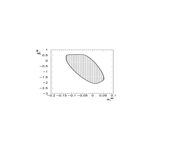
FIG. 1.: 99% CL allowed region for the parameters $\alpha_{1}^{NC}$ and $\beta_{1}^{NC}$ for for $\Lambda=1$ TeV and $160$ GeV $\leq m_{\text{{top}}}\leq 190$ GeV and $\mu=m_{\text{{top}}}$.

REFERENCES

• [1] LEP Electroweak Working Group, contributions to the 28th Int. Conf. on High-energy Phys., Warsaw, Poland, 1996, CERN-PPE/96-183 (1996).
• [2] D. Gerdes for CDF and D0 Collaborations, hep-ex/9609013.
• [3] R. D. Peccei and X. Zhang, Nucl. Phys. B337 (1990) 269.
• [4] W. A. Bardeen, C. T. Hill and M. Lindner, Phys. Rev. D41 (1990) 1647.
• [5] E. Malkawi and C.–P. Yuan, Phys. Rev. D 50 (1994) 4462; D. O. Carlson, E. Malkawi, and C.–P. Yuan, Phys. Lett. B337 (1994) 145.
• [6] G. Altarelli, preprint CERN–TH/96–265 (hep-ph/9611239); G. Altarelli, and F. Caravagios private comunication.
• [7] T. Appelquist and C. Bernard, Phys. Rev. D22 (1980) 200; A. Longhitano, Phys. Rev. D22 (1980) 1166; Nucl. Phys. B188 (1981) 118.
• [8] M. S. Chanowitz, M. Golden, and H. Georgi, Phys. Rev. D36 (1987) 1490.
• [9] F. Larios and C.–P, Yuan, Phys. Rev. D55 (1997) 7218; H.–J. He, Y.–P. Kuang, and C.–P. Yuan, preprint DESY-97-056 (hep-ph/9704276).
• [10] G. J. Gounaris, F. M. Renard, and C. Verzegnassi, Phys. Rev. D52 (1995) 451.
• [11] J. Wudka, in the Proceedings of the IV Workshop on Particles and Fields of the Mexican Physical Society (hep-ph/9405206).
• [12] S. Dittmaier, C. Grosse-Knetter, Nucl. Phys. B459 (1996) 497.
• [13] G. Altarelli, R. Barbieri, and F. Caravaglios, Nucl. Phys. B405 (1993) 3.
• [14] J. Bernabeu, A. Pich, and A. Santamaria, Phys. Lett. B200 (1988) 569.
• [15] C. G. Bollini and J. J. Giambiagi, Phys. Lett. B40 (1972) 566; G. ’t Hooft and M. Veltman, Nucl. Phys. B44 (1972) 189; J. F. Ashmore, Nuov. Cim. Lett. 4 (1972) 289.