The Preheating - Gravitational Wave Correspondence: I

Abstract

The gravitational wave equations form a parametric resonance system during oscillatory reheating after inflation, when cast in terms of the electric and magnetic parts of the Weyl tensor. This is in direct analogy with preheating. For chaotic inflation with a quadratic potential, this analogy is exact. The resulting amplification of the gravitational wave spectrum begins in the broad resonance regime for chaotic inflation but quickly moves towards narrow resonance. This increases the amplitude and breaks the scale invariance of the tensor spectrum generated during inflation, an effect which may be detectable. The parametric amplification is absent, however, in 1st-order phase transition models and “warm” inflationary models with continuous entropy production.

I Introduction

Standard inflation ends with the universe in a near-vacuum state & hence reheating the universe successfully is a crucial requirement of inflationary scenarios. A full theory of this phoenix-like revival from the remains of the inflaton field remains elusive given the complexities of non-equilibrium field theory on curved spacetime, although the so-called elementary theory has been known for over a decade and a half [1, 2, 37]. However, whereas previously the importance of parametric resonance was recognised [2, 4], it was not studied in the broad-resonance realm. It was essentially the move into this non-perturbative regime - preheating - which lead to a radical paradigm shift [3], demonstrating that inflation may give rise to nonlinear fluctuations of sufficient magnitude to restore symmetries [14] and offer a way of gracefully exiting inflation [15]. In addition, it has forced the study of backreaction phenomena [3, 16] using nonperturbative methods, and the effects of scattering during the broad resonance regime [21, 20].

However, the implications of oscillatory reheating (through a second order phase transition) and the resulting large quantum fluctuations for local curvature (metric) fluctuations has been largely unexplored until now, and limited to scalar modes [28, 29, 30]. The evolution of the tensor (gravitational wave) spectrum has essentially been completely ignored, apart from a recent study of gravitational bremstrahlung generated through the interactions of the large quantum fluctuations in the inflaton and decay-product fields [6]. Gravitational wave production during the bubble-wall collisions of a first order phase transition have been rather more studied [5]. However, the gravitational waves produced in these mechanisms are backreaction phenomena, since they are due to the scalar field fluctuations, rather than the background zero mode evolution itself.

In this paper we wish to demonstrate that there exists such an amplification of gravitational waves, essentially due to the oscillation of the zero mode of the inflaton during reheating. This is in addition to any gravitational bremstrahlung that may be produced by the associated scalar fluctuations. Further, we show that a direct analogy exists in the treatment of preheating and gravitational wave evolution at the end of inflation if this occurs via a second order phase transition, as we shall assume here. Indeed, both are governed by (approximately) Floquet systems . In the case of the quadratic potential, $V(\phi)=\frac{1}{2}m_{\phi}^{2}\phi^{2}$, both preheating and gravitational wave amplification are initially well approximated by the Mathieu equation, hence the correspondence of the title. This “duality” is exhibited using the covariant Maxwell-Weyl form of the Einstein field equations (see section II and e.g. [8]), and is partially hidden in the Bardeen formalism [18]. This demonstration of gravitational wave amplification should be considered in the light of the controversy surrounding tensor amplification during instantaneous phase transitions. In these models, two different cosmologies such as de Sitter and radiation Friedmann-Lemaître-Robertson-Walker (flrw) are matched across a single 3-space through appropriate junction conditions. Such discussions are indeed rather technical and subtle, dealing with discontinuities in the Einstein field equations, and do not model the actual physics of reheating. Further, there is as yet no absolute clarity as to the possibility of tensor amplification in these models, with claims both for [10] and against [11, 12] amplification.

Now, in the covariant approach to cosmology (see e.g. [8, 36, 13]), a fundamental vector is the four velocity of the fluid, $u^{a}$, which is used to perform a $3+1$ splitting of spacetime. The expansion, $\Theta$, is then defined via:

$$\Theta=u^{a}{}_{;a}$$ (1)

where ; denotes the covariant derivative. In flrw universes, $\Theta=3\dot{S}/S=3H$, where S is the scale factor and H is the Hubble constant. In the case of a minimally coupled inflaton field $\phi$, we may choose our $u^{a}$ to be proportional to the timelike vector field orthogonal to the surfaces of constant $\phi$, i.e. proportional to the covariant derivative $\phi_{;a}$ [9], with $h_{ab}=g_{ab}+u_{a}u_{b}$ the projection tensor into the orthogonal 3-spaces. The convective time derivative is defined as $\dot{Q}^{a..b}\equiv Q^{a..b}{}_{;c}u^{c}$, for arbitrary $Q^{a..b}$, i.e. it is the covariant derivative projected along the four velocity. This coincides with the usual time derivative in flrw spacetimes. The evolution equation for the inflaton $\phi$, with effective potential $V_{\mbox{eff}}(\phi)$ , is given by:

$$\ddot{\phi}+\Theta\dot{\phi}+V^{\prime}_{\mbox{eff}}(\phi)+\Pi\phi=0$$ (2)

where ${}^{\prime}\equiv\partial/\partial\phi$. $\Pi$ in eq. (2) generically represents the backreaction of quantum fluctuations on the zero mode evolution via a change to the effective mass of the inflaton. It may be written specifically as the polarisation operator [37] or given explicitly in certain approximations, such as Hartree factorisation [15], or the large-$N$ limit of $O(N)$ vector models [16].

The geometry of space (if the background is flrw) enters only through the expansion $\Theta$, whose evolution is given by the Raychaudhuri equation [8], which in flat flrw spacetime is:

$$\dot{\Theta}=-\frac{3\kappa}{2}\dot{\phi}^{2}$$ (3)

Here $\kappa=8\pi$ is the gravitational coupling constant.

To illustrate preheating and hence the first axis of the correspondence between reheating and gravitational wave evolution, assume that $\phi$ interacts with a light scalar field $\chi$, which itself has no self-interaction, via the Lagrangian interaction term $\frac{1}{2}g^{2}\phi^{2}\chi^{2}$. Consider the simplest effective potential for chaotic inflation:

$$V(\phi)=\frac{1}{2}m_{\phi}^{2}\phi^{2}\,.$$ (4)

The solution of the inflaton equation of motion (2), when the frequency is an adiabatic invariant, is that of decaying sinusoidal oscillations, $\phi(t)=\Phi(t)\sin(m_{\phi}t)$. In the absence of particle production the amplitude varies roughly as $\Phi\sim\frac{1}{m_{\phi}t}$, due to the averaged expansion. The time evolution of the quantum fluctuations for each mode of the $\chi$-field is given by (neglecting $m_{\chi}$) [3]:

$$\ddot{\chi}_{k}+\Theta\dot{\chi}_{k}+\left(\frac{k^{2}}{S(t)^{2}}+g^{2}\Phi^{2}\sin^{2}(m_{\phi}t)\right)\chi_{k}=0$$ (5)

This can be put in canonical Mathieu form if one neglects the expansion of the universe ($\Theta=0$):

$$\chi_{k}^{\prime\prime}+\left[A(k)-2q\cos(2z)\right]\chi_{k}=0$$ (6)

with dimensionless coefficients:

$$A_{\chi}(k)=\frac{k^{2}}{m_{\phi}^{2}S^{2}}+2q~{}~{},~{}~{}~{}~{}q_{\chi}=\frac{g^{2}\Phi^{2}}{4m_{\phi}^{2}}$$ (7)

and $z=m_{\phi}t$. Depending on the size of the coupling, $g$, and the mass $m_{\phi}$, certain modes $\chi_{k}$ will thus be amplified exponentially: $\chi_{k}=p_{k}(m_{\phi}t)\exp(\mu_{k}{}^{(n)}m_{\phi}t)$, where $p_{k}$ are functions with the same period as the oscillations of the inflaton field and the positive $\mu_{k}{}^{(n)}$ are the Floquet indices corresponding to the $n$-th instability band. The existence of resonance bands survives when the expansion of the universe is included [19, 15]. The parameter $q$ divides the phase space into three broad classes with qualitatively different behaviour. The case $q\ll 1$ is well understood [4] and can be treated perturbitively, the effects of expansion being important. The broad resonance case is described roughly by $\pi^{-1}<q<q_{*}~{},~{}q_{*}\sim 10^{2}$, is non-perturbative and requires consideration of the backreaction of created particles on the zero mode $\phi_{0}$. The resonance bands are characterized by huge occupation numbers of produced particles, typically of order $n_{k}\sim\frac{1}{g^{2}}$. The upper limit, $q_{*}$, is for an expanding universe and is much lower in Minkowski spacetime ($\Theta=0$) [21]. The wide resonance, $q\gg q_{*}$, evolution is dominated by scattering effects which rapidly shut-off the exponential growth of the $\chi$ fluctuations [20, 21].

II Gravitational waves in Maxwell-Weyl form

Gravitational waves (tensor perturbations) describe curvature fluctuations unassociated directly with matter. We will discuss their evolution using the elegant covariant formalism [8].

The covariant derivative of the four velocity $u_{a}$ is split into kinematic parts via:

$$u_{a;b}=\sigma_{ab}+\omega_{ab}+\frac{1}{3}\Theta h_{ab}-\dot{u}_{a}u_{b}$$ (8)

where the shear $\sigma_{ab}=\sigma_{(ab)}$ is traceless, $\omega_{ab}=\omega_{[ab]}$ is the vorticity and $h_{ab}=g_{ab}+u_{a}u_{b}$ is both the projection tensor into, and the metric of, the hypersurfaces orthogonal to $u_{a}$ in the case where $\omega_{ab}=0$ . $\dot{u}_{a}$ is the acceleration and is caused by pressure gradients. Here indices surrounded by round brackets denote symmetrization on those indices while square brackets denote anti-symmetrization.

A The Electric and Magnetic Weyl Tensors

A purely tensor description of gravitational waves is still partially lacking in the covariant approach [36], but a sufficient description was given first by Hawking (1966) [7] in terms of the magnetic $H_{ab}$ and electric, $E_{ab}$ parts of the Weyl tensor, which are automatically traceless and gauge-invariant (since they vanish in exactly flrw spacetimes) [13, 8], given by:

$$H_{ac} = \frac{1}{2}\eta_{ab}{}^{gh}C_{ghcd}u^{b}u^{d}~{}~{}\equiv{}^{*}\!C_{abcd}u^{b}u^{d}$$ (9)

$$E_{ac} = C_{abcd}u^{b}u^{d}$$ (10)

where $*$ is the usual dual (Hodge) operator. These definitions are completely analogous to those of the electric and magnetic fields in terms of the field strength, $F_{ab}$, in standard electromagnetism [22]. A natural interpretation of the electric Weyl part is given by the geodesic deviation equations, which for the special case of a plane gravitational wave propagating along the $x^{1}$ direction are: [24]

$$\ddot{\xi}^{\alpha}=E^{\alpha}{}_{\beta}\xi^{\beta}~{}~{},~{}~{}~{}\alpha,\beta=2,3$$ (11)

where $\xi^{\alpha}$ is the connecting vector between orthonormal tetrads associated with the congruence of null geodesics ruled by gravitons. This means that we can directly attribute the physical effects of linear tensor perturbations, on e.g. a gravitational wave detector, to the electric part of the Weyl tensor.

The evolution equations for $H_{ab}$ and $E_{ab}$ are provided by the Bianchi identities:

$$R_{ab[cd;e]}=0\Longleftrightarrow C^{abcd}{}_{;d}=R^{c[a;b]}-\frac{1}{6}g^{c[a}R^{;b]}~{},$$ (12)

with the above equivalence only holding in four dimensions. These yield the nonlinear gravitational analogues of the Maxwell equations [8] which take the form of two evolution equations, $\dot{E}_{ab},\dot{H}_{ab}$ and two constraint equations, $\mbox{div}E_{ab},~{}\mbox{div}H_{ab}$ - see equations (A2), (A4), (A7), (A8), again just as in the case of Maxwell’s equations.

In addition we can associate a natural super-energy to gravitational waves in the covariant approach through the scalar:

$$E_{ab}E^{ab}+H_{ab}H^{ab}~{},$$ (13)

which is in fact just the $u_{a}$-projected timelike component of the Bel-Robinson tensor, the super-stress-tensor for the gravitational field [25, 26]. After expansion in eigenfunctions of the tensor Helmholtz equation, and using the relation $\nabla^{2}=-k^{2}/S^{2}$, the modes $H_{k}$, of the magnetic part $H_{ab}$ satisfy (see [13] and appendix A for the derivation):

$$\ddot{H}_{k}+\frac{7}{3}\Theta\dot{H}_{k}+\left[\frac{k^{2}}{S^{2}}+\dot{\Theta}+\Theta^{2}+\frac{1}{2}(\mu-p)\right]H_{k}=0~{},$$ (14)

where $\mu$ and $p$ are the relativistic energy density and pressure respectively. This is a simple decoupled equation (c.f. eq. 5), while the shear satisfies:

$$\ddot{\sigma}_{k}+\frac{5}{3}\Theta\dot{\sigma}_{k}+\left[\frac{k^{2}}{S^{2}}+\frac{\Theta^{2}}{9}+\frac{1}{6}\mu-\frac{3}{2}p\right]\sigma_{k}=0~{}.$$ (15)

Finally the modes of the electric part obey an equation which is coupled to the shear (c.f. equation A2):

$$\ddot{E}_{k} + \frac{7}{3}\Theta\dot{E}_{k}+\left[\frac{k^{2}}{S^{2}}+\dot{\Theta}+\Theta^{2}+\frac{1}{2}(\mu-p)\right]E_{k}$$ (16)

$$= -\left[\frac{1}{3}\Theta(\mu+p)+\frac{1}{2}(\dot{\mu}+\dot{p})\right]\sigma_{k}$$ (17)

The shear can be eliminated from the $E_{k}$ equation by another differentiation [13], but since the shear is the variable which appears in the covariant formula for the temperature anisotropies of the CMB, it will be convenient to retain it explicitly. The shear does not appear in the $E_{ab}$ equation when $\mu+p=0$, i.e. in exact de Sitter spacetime or in vacuum, be it Minkowski ($\Theta=0$) or Milne ($\Theta\not=0$). In this case there is an exact symmetry between the equations (14,17) under the interchange $E_{ab}\leftrightarrow H_{ab}$. This is the linearised version of the exact nonlinear rotational duality that exists in the full vacuum Bianchi identities [38] and which is the gravitational analogue of the electromagnetic duality in vacuum [39] which lead to the Montonen-Olive conjecture and the modern progress in dualities of supersymmetry and string theory [40]. See [22, 23] for further analysis of the gravity-electromagnetic duality in cosmology.

1 Oscillatory dynamics in reheating

Now let us specialise equations (14-17) to the case of classical scalar field dynamics. Treating here only the case of a single scalar field, we have, using the equivalence of $\phi$ with a perfect fluid:

$$\mu=\kappa\left[\frac{1}{2}\dot{\phi}^{2}+V(\phi)\right]~{},~{}~{}p=\kappa\left[\frac{1}{2}\dot{\phi}^{2}-V(\phi)\right]$$ (18)

so that

$$\frac{1}{2}(\mu-p)=\kappa V(\phi),~{}~{}(\mu+p)=\kappa\dot{\phi}^{2}~{},~{}~{}(\dot{\mu}+\dot{p})=2\kappa\dot{\phi}\ddot{\phi}~{}.$$ (19)

Here $V(\phi)$ is the effective potential of the scalar field. Note that if scalar perturbations become important then these relations will gather terms proportional to $(\nabla\phi)^{2}$ [27]. This is precisely the case if one wishes to consistently study the production of tensor perturbations from gravitational bremstrahlung [6]. However, it brings with it a host of complexities, since for example, eq.s (14 - 17) must be rederived in the presence of the backreaction of matter fluctuations, a highly non-trivial problem. We will not consider this issue further here.

The important point is that with the above identifications, the equations (14), (15), (17) become generalizations of eq.(5). There thus exists a strong connection between the evolution governing reheating under a given potential and the equations governing the evolution $H_{k},E_{k}$ and $\sigma_{k}$ particularly when $V(\phi)$ is an even polynomial in $\phi$, as in chaotic inflation.

III Chaotic inflation and Duality

Consider again the quadratic chaotic potential, Eq. (4). In addition to chaotic inflation, this describes the dynamics of the invisible axion, and the Polonyi and moduli fields of supergravity and string theory, with appropriate changes to the values of the masses, $m^{2}\equiv V^{\prime\prime}(\phi)$.

Here we will neglect the expansion of the universe as before to delineate the duality [19]. This would of course not be adequate for the study of long-time oscillatory amplification, but is justified if the period of oscillations of $\phi$ is small compared with typical averaged expansion times, i.e. $m_{\phi}\gg\overline{\Theta}$. However, the oscillations of the expansion rate should also be included in a full description [18] which will act as an additional source of resonance. This will be important in obtaining the tensor spectrum from oscillating cold dark matter (CDM) relics like the invisible axion [31]. The equation (14) for the modes, $H_{k}$, of the magnetic part $H_{ab}$ now becomes:

$$\ddot{H}_{k}+\left(\frac{k^{2}}{S^{2}}+\frac{\kappa m_{\phi}^{2}}{2}\Phi^{2}\sin^{2}(m_{\phi}t)\right)H_{k}=0$$ (20)

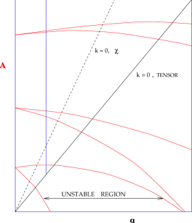
FIG. 1.: A schematic of the instability chart for the Mathieu equation. The two diagonal lines correspond respectively to the zero-modes ($k=0$) of the gravitational wave spectrum and the $\chi$-spectrum of eq. (4), for the case $g^{2}<m_{\phi}^{2}$. The vertical line near the left border of the chart is a sample spectrum for a given model (i.e. value of $q$).

This is the Mathieu equation and is precisely the same as equation (5) for the evolution of the quantum fluctuations $\chi_{k}$, with the replacement $g^{2}\rightarrow\kappa\frac{m^{2}_{\phi}}{2}=4\pi m^{2}_{\phi}$. Hence $q_{H}=\pi\Phi$. The requirement that production of $\chi$ bosons is more efficient than $H_{ab}$ amplification is then $g^{2}>4\pi m_{\phi}^{2}$. If $m_{\phi}\sim 10^{-6}$, as required to match CMB observations [32], then this is a weak constraint on the coupling $g$, namely $g^{2}>10^{-11}$. Nevertheless, it is a constraint independent of $\Phi$ and hence applies to both chaotic and new inflationary models (which have quadratic potentials near the global minima). If the constraint is not met, it implies that reheating occurs preferentially via production of gravitons rather than the $\chi$-channel .

In figure 1 this situation is depicted schematically on the instability chart of the Mathieu equation: namely, the situation in which $q_{H}>q_{\chi}$. The two diagonal lines corresponding to the mode $k=0$, delimit the physical (i.e. upper) region of the chart. The single vertical line corresponds to a sample spectra for a given value of $q$. Note that for this value of $q$, the tensor spectrum has modes in the first fundamental resonance band, while there are no $\chi$ modes which lie in this band. Figure (2) shows a numerical integration of the spectrum as a function of time for modes in both stable and unstable bands. Figure (3) zooms in on the spectrum within a stable band.

Can $H_{ab}$ be amplified in the broad resonance regime ? This is necessary if gravitational wave enhancement is to be really effective over the expansion. This requires $q_{H}>\pi^{-1}$. Since $q_{H}=\pi\Phi^{2}$ this implies $\Phi>\pi^{-1}$ in units of the Planck energy. In the case of chaotic inflation, the amplitude of oscillations goes as [33] $\Phi\sim 1/N$, where $N$ is the number of oscillations of $\phi$, neglecting the non-equilibrium backreaction at the end of preheating which often leads to a sudden decrease in $\Phi$ [16]. Thus during preheating proper, $q_{H}\sim\pi/N^{2}$, and $H_{ab}$ is initially amplified in the broad resonance regime, but moves rapidly towards narrow resonance.

	$\chi_{k}$	$H_{k}$	$\sigma_{k}$
A	$\frac{k^{2}}{S^{2}m_{\phi}^{2}}+2q$	$\frac{k^{2}}{S^{2}m_{\phi}^{2}}+2q$	$\frac{k^{2}}{S^{2}m_{\phi}^{2}}+\frac{2}{19}q$
q	$\frac{g^{2}\Phi^{2}}{4m_{\phi}^{2}}$	$\pi\Phi^{2}$	$\frac{19}{6}\pi\Phi^{2}$

Consider now the equations for the electric Weyl field, $E_{ab}$, and the shear $\sigma_{ab}$. They form a partially decoupled linear system with time-dependent coefficients that form an approximately Floquet system. Here we ignore the decay of the amplitude. This is appropriate during preheating while the non-equilibrium effects and backreaction of graviton production are not too strong and the oscillation period of $\phi$, (controlled by $m_{\phi}$) is short compared with the expansion time scale. This gives:

$$\ddot{E}_{k}+\left(\frac{k^{2}}{S^{2}}+\frac{m_{\phi}}{2}\Phi^{2}\sin(m_{\phi}t)\right)E_{k}=\frac{1}{8}\left[\Phi^{2}m_{\phi}^{3}\sin(2m_{\phi}t)\right]\sigma_{k}$$ (21)

with

$$\ddot{\sigma}_{k}+\left(\frac{k^{2}}{S^{2}}-\kappa\frac{3}{4}\dot{\phi}^{2}+\kappa\frac{5}{6}m_{\phi}^{2}\phi^{2}\right)\sigma_{k}=0$$ (22)

The equation for the shear can again be cast in the form of the Mathieu equation with

$$A(k)_{\sigma}=\frac{k^{2}}{m_{\phi}^{2}S^{2}}+\frac{2}{19}q_{\sigma}~{}~{},~{}~{}~{}q_{\sigma}=\kappa\frac{19}{48}\Phi^{2}~{}.$$ (23)

A comparison of parameters is given in table 1.

Note that the shear always lies in a region of broader resonance than the magnetic part of the Weyl tensor because $q_{\sigma}>q_{H}$ and $A_{\sigma}(k)<A_{H}(k)$. Now $q_{\sigma}=\frac{19\pi}{6}\Phi^{2}$ with the requirement of broad resonance amplification of the shear $\Phi>\sqrt{\frac{6}{19}}\pi^{-1}\sim 0.56\pi^{-1}\sim 0.18$.

Since it is the shear which directly determines the tensor contribution to the anisotropy of the CMB, this may allow one to place constraints on large-amplitude oscillatory reheating. Since power-law inflation is known to produce one of the strongest tensor signals during slow-roll [42] the signal to noise (due to cosmic variance and instrument) ratio for the tensor component in the CMB may be significantly larger than previously hoped [43]. The CMB anisotropy from a tensor signal is [34, 35]:

$$\left(\frac{\delta T}{T}\right)^{*}=-\int_{E}^{R}S~{}\sigma_{ab}~{}k^{a}k^{b}d\lambda$$ (24)

The left hand side is a gauge-invariant measure of the anisotropy in the CMB, and $k^{a}$ is the wave vector ruling our past null cone.

Now for purely tensor perturbations, $\sigma_{ab}$ and $E_{ab}$ are related by [13]:

$$\dot{\sigma}_{ab}=-\frac{2}{3}\Theta\sigma_{ab}-E_{ab}$$ (25)

we see that exponential growth of the shear implies exponential growth of the electric Weyl field, and hence the energy in gravitational waves, $\Omega_{GW}$, increases exponentially, via eq. (13).

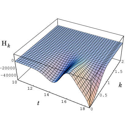
FIG. 2.: The gravitational wave spectrum, $H_{k}$ as a function of $k$ and $t$, with the initial condition $H(0)=0,\dot{H}(0)=10^{-4}$ and starting in the broad resonance regime. As can be seen, the power spectrum becomes highly $k$-dependent, breaking the usual scale-invariance of the envelope predicted by inflation. Further, the amplitude of the spectrum is exponentially enhanced by resonant reheating over its value during inflation.

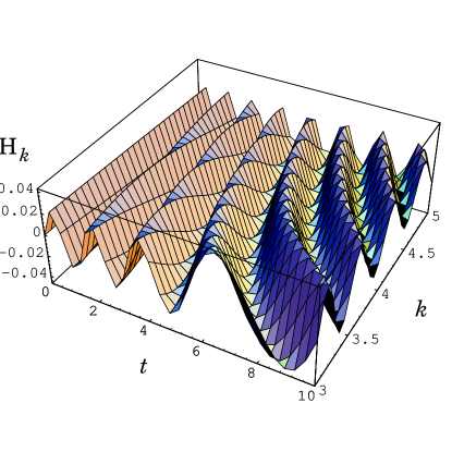
FIG. 3.: A zoom of the stable band region $3\leq k\leq 5$. The solution is the usual bounded oscillatory one. Note the scale on the $z$-axis (c.f. fig. 2).

However, a counter example to the above situation occurs if there is non-thermal symmetry restoration [14, 16]: start with $\phi\gg M_{pl}$, as in the chaotic inflation scenario, but with a Coleman-Weinberg type new-inflationary potential, which is flat near the origin. If preheating restores symmetry, a phase of new inflation begins with $\phi=0$. This redshifts away the resonantly amplified tensor spectrum. The second stage of reheating will be much less effective in amplifying the tensor spectrum than the first if $V(0)\ll M_{pl}^{4}$. This is the generic case for non-thermal symmetry restoration and hence amplification will occur in the very narrow resonance region where expansion effects are expected to dominate, leaving an almost untouched, scale-invariant tensor spectrum.

IV Conclusions

The main result of this paper is that gravitational wave perturbations can be naturally amplified during a second order phase transition. Thus, in addition to the standard creation of a scale-invariant stochastic gravitational wave spectrum due to quantum fluctuations during inflation, there may be amplification of this spectrum during reheating which breaks the scale invariance and may significantly enhance the rms amplitude of the tensor perturbation spectrum with no a priori limit on the maximum wavelength affected. However the exact pattern and size of this “symmetry breaking” is highly model dependent, and is hence relevant to inflationary potential reconstruction attempts [42, 43]. This amplification is qualitatively different from gravitational bremstrahlung [6] since it is due to the coherent oscillation of the mean energy density and pressure of the inflaton, and is largely insensitive to the nature of the scalar field fluctuations.

We have further examined chaotic inflation with a quadratic potential in detail and found a duality between the equations describing the growth of $\chi$ fluctuations and those of the magnetic part of the Weyl tensor and the shear, the latter being the variable which determines the gravitational wave signal in the CMB; eq (24). Finally, the resonant enhancement of the tensor spectrum is completely missing in those models of inflation which involve a continuous production of entropy during inflation, such as in the “warm” inflation models [44]. Future work will examine the quantitative importance of expansion, quantum backreaction and scattering effects for the amplification of gravitational waves, and will compare the Weyl formalism with the more typical Bardeen approach.

Acknowldegements

It is a pleasure to thank George Ellis, Andre Linde, Claudio Scrucca, Stefano Liberati, Roy Maartens and Peter Dunsby for discussions and Andre Linde for pointing out that the idea of resonant gravity wave amplification due to the oscillation of the expansion had been worked on, though previously unpublished.

A Derivation of the wave equations

The Bianchi identities, eq. (12), yield the following evolution equations [13]:

$$h^{m}{}_{a}h^{t}{}_{c}\dot{E}^{ac}+J^{mt}-2H_{a}{}^{(t}\eta^{m)bpq}u_{b}\dot{u}_{p}+h^{mt}\sigma^{ab}E_{ab}+$$ (A1)

$$+\Theta E^{mt}-3E_{s}{}^{(m}\sigma^{t)s}-E_{s}{}^{(m}\omega^{t)s}=-\frac{1}{2}(\mu+p)\sigma^{tm}\,,$$ (A2)

the ‘$\dot{E}$’ equation, $h_{ab}=g_{ab}+u_{a}u_{b}$ is the projection tensor into the hypersurfaces orthogonal to $u_{a}$, and

$$h^{m}{}_{a}h^{t}{}_{c}\dot{H}^{ac}-I^{mt}+2E_{a}{}^{(t}\eta^{m)bpq}u_{b}\dot{u}_{p}+h^{mt}\sigma^{ab}H_{ab}+$$ (A3)

$$+\Theta H^{mt}-3H_{s}{}^{(m}\sigma^{t)s}-H_{s}{}^{(m}\omega^{t)s}=0$$ (A4)

is the ‘$\dot{H}$’ equation, where we have given only the perfect fluid form, and where the covariant curl terms are defined as:

$$J^{mt} = h_{a}{}^{(m}\eta^{t)rsd}u_{r}H^{a}{}_{s;d}$$ (A5)

$$I^{mt} = h_{a}{}^{(m}\eta^{t)rsd}u_{r}E^{a}{}_{s;d}$$ (A6)

These are the fully nonlinear equations and despite their complexity, note the symmetries between the equations (A2) and (A4), broken only by the driving term $-\frac{1}{2}(\mu+p)\sigma_{ab}$ in eq. (A2) which is absent in the $\dot{H}_{ab}$ equation. In addition there are the gravitational ‘div E’ and ‘div H’ constraint equations:

$$h^{t}{}_{a}E^{as}{}_{;d}h^{d}{}_{s}-\eta^{tbpq}u_{b}\sigma^{d}{}_{p}H_{qd}+3H^{t}{}_{s}\omega^{s}=\frac{1}{3}h^{tb}\mu_{;b}\,,$$ (A7)

$$h^{t}{}_{a}H^{as}{}_{;d}h^{d}{}_{s}+\eta^{tbpq}u_{b}\sigma^{d}{}_{p}E_{qd}-3E^{t}{}_{s}\omega^{s}=(\mu+p)\omega^{t}\,,$$ (A8)

where the vorticity vector is $\omega^{a}=\frac{1}{2}\eta^{abcd}u_{b}\omega_{cd}$.

In linear theory about a flrw background, to specify that we are interested in purely tensor, i.e. gravitational wave solutions, we require that there are no scalar or vector perturbations:

$$\frac{1}{3}h_{a}{}^{b}\mu_{;b}=\omega_{a}=0$$ (A9)

Examining equations (A7,A8) and dropping all second order terms, this implies that the divergences themselves vanish:

$$h^{t}{}_{a}E^{as}{}_{;d}h^{d}{}_{s}=h^{t}{}_{a}H^{as}{}_{;d}h^{d}{}_{s}=0$$ (A10)

This ensures only purely radiative solutions, and since $E^{a}{}_{a}=H^{a}{}_{a}=0$, by the construction of the Weyl tensor, we have the analogue of the transverse-traceless (TT) conditions usually imposed on tensor metric perturbations.

The equations (A2,A4) can be linearised consistently [13], giving the coupled set:

$$\dot{E}_{ab}+\Theta E_{ab}+h_{(a}^{f}\eta_{b)cde}u^{c}\nabla^{e}H_{f}^{d}+\frac{1}{2}(\mu+p)\sigma_{ab}=0$$ (A11)

and

$$\dot{H}_{ab}+\Theta H_{ab}-h_{(a}^{f}\eta_{b)cde}u^{c}\nabla^{e}E_{f}^{d}=0$$ (A12)

These can be converted to wave equations for $E_{ab}$ and $H_{ab}$ by differentiation (see [13]). Similarly the shear, $\sigma_{ab}$, satisfies a wave equation and the three variables form a partially - coupled system. Once one transforms the variables to momentum space via expansion in eigenfunctions, $Q^{k}_{ab}$, of the tensor Helmholtz equation, one obtains the ordinary differential equations (14), (15), (17).

REFERENCES

- [1] A.D. Dolgov and A.D. Linde, Phys. Lett. 116B, 329 (1982); L.F. Abbott, E. Fahri, and M. Wise, Phys. Lett. 117B, 29 (1982).
- [2] J. Traschen and R. Brandenberger, Phys. Rev. D 42, 2491 (1990); A.D. Dolgov and D.P. Kirilova, Sov. Nucl. Phys. 51, 273 (1990).
- [3] L. Kofman, A. Linde, and A. A. Starobinsky, Phys. Rev. Lett. 73, 3195 (1994)
- [4] Y. Shtanov, J. Traschen and R. Brandenberger, Phys. Rev. D 51, 5438 (1995)
- [5] M. Kamionkowski, A. Kosowsky, and M. S. Turner, Phys. Rev. D 49, 2837 (1994); astro-ph/9310044
- [6] S. Yu. Khlebnikov, I. I. Tkachev, hep-ph/9701423 (1997)
- [7] S. W. Hawking, Ap. J. 145, 544 (1966)
- [8] G. F. R. Ellis, Relativistic Cosmology, in Cargése Lectures in Physics, vol. VI, ed. E. Schatzmann (Gordon and Breach, 1973), p.1
- [9] M. Bruni, P. K. S. Dunsby and G. F. R. Ellis, Class. Quant. Grav. 9, 921 (1992)
- [10] L. P. Grishchuk, Phys. Rev. D 53, 6784, (1996) ; ibid 50, 7154 (1994)
- [11] N. Deruelle and V. F. Mukhanov, Phys. Rev. D 52, 5549 (1995)
- [12] J. Martin and D. J. Schwarz, gr-qc/9704049 (1997)
- [13] P. K. S. Dunsby, B. A. Bassett and G. F. R. Ellis, Class. Quant. Grav., 14, 1215 (1997)
- [14] L. Kofman, A. Linde and A. A. Starobinsky, Phys. Rev. Lett. 76, 1011 (1996)
- [15] D. Boyanovsky, D. Cormier, H.J. de Vega, R. Holman, Phys. Rev. D 55, 3373 (1997), D. Boyanovsky, D. Cormier, H. J. de Vega, R. Holman, A. Singh, M. Srednicki, hep-ph/9703327 (1997)
- [16] D. Boyanovsky, H. J. de Vega, R. Holman, J. F. J. Salgado, Phys.Rev. D 54, 7570 (1996); D. Boyanovsky, H.J. de Vega, R. Holman, D.S. Lee, and A. Singh, Phys.Rev. D 51, 4419 (1995); D. Boyanovsky, M. D’Attanasio, H. J. de Vega, R. Holman, D.-S. Lee, and A. Singh, Phys. Rev. D 52, 6805 (1995)
- [17] M. Yoshimura, Prog. Theo. Phys. 94, 873 (1995); H. Fujisaki, K. Kumekawa, M. Yamaguchi, and M. Yoshimura, Phys. Rev. D 53, 6805 (1995)
- [18] B. A. Bassett, in preparation (1997)
- [19] D. Kaiser, Phys. Rev. D 53, 1776 (1996); D. Kaiser, hep-ph/9702244 (1997)
- [20] S. Yu. Khlebnikov, I. I. Tkachev, hep-ph/9610477 and hep-ph/9608458, (1996) and S. Yu. Khlebnikov, I. I. Tkachev, Phys. Rev. Lett. 77, 219 (1996)
- [21] T. Prokopec, T. G. Roos, hep-ph/9610400 (1996)
- [22] G. F. R. Ellis and P. Hogan, Gen. Rel. Grav. 29, 235 (1996)
- [23] W. B. Bonnor, Class. Quant. Grav. 12, No 2, 499 (1995), & ibid, 12 No 6, 1483 (1995)
- [24] F. de Felice and C. J. S. Clarke Relativity on Curved Manifolds, (Cambridge Univ. Press, 1990)
- [25] V. D. Zakharov, Gravitational Waves in Einstein’s Theory, Trans. R. N. Sen, (Halsted, New York, 1973).
- [26] B. Mashoon, J.C. McClune and H. Quevedo, Preprint, gr-qc/9609018 (1996)
- [27] E. W. Kolb and M. S.Turner, The Early Universe (Addison-Wesley, 1990)
- [28] T. Hamazaki and H. Kodama, gr-qc/9609036 (1996); H. Kodama and T. Hamazaki, gr-qc/9608022 (1996))
- [29] Y. Nambu and A. Taruya, gr-qc/9609029 (1996)
- [30] A. Linde and V. Mukhanov, astro-ph/9610219 (1996)
- [31] J.E. Kim, Physics Reports, 150, 1 (1987)
- [32] D.S. Salopek, Phys. Rev. D, 43, 3214 (1991)
- [33] A. D. Linde, in lectures of the School for Astrofundamental Physics, (Erice, 1996)
- [34] H. Russ, M. Soffel, C. Xu and P.K.S. Dunsby, Phys. Rev. D, 48, 4552 (1993)
- [35] P. K. S. Dunsby, UCT Preprint, A fully covariant description of CMB anisotropies , (1997)
- [36] R. Maartens, G. F. R. Ellis and S. T. C. Siklos, Class. Quant. Grav. 14, (1997) gr-qc/9611003; R. Maartens, Phys. Rev. D 55, 463 (1997)
- [37] A.D. Linde, Particle Physics and Inflationary Cosmology (Harwood, Chur, Switzerland, 1990).
- [38] R. Maartens and B. A. Bassett, gr-qc/9704059 (1997)
- [39] C. Montonen and D. I. Olive, Phys. Lett. 72 B, 117, (1977)
- [40] N. Seiberg and E. Witten, Nucl. Phys. B 426, 19 (1994); Erratum B 430, 485 (1994)
- [41] D. H. Lyth and E. D. Stewart, Phys. Rev. Lett. 75, 201 (1995); D. H. Lyth and E. D. Stewart, Phys. Rev. D 53 1784 (1996)
- [42] J.E. Lidsey et al, astro-ph/9508078, (1995)
- [43] L. Knox and M.S. Turner, Phys. Rev. Lett. 73, 3347 (1994)
- [44] A. Berera, Phys. Rev. D 54, 2519, (1996)