Aspects of Neutrino Detection
of Neutralino Dark Matter
Joakim Edsjö111E-mail address: edsjo@teorfys.uu.se
Department of Theoretical Physics, Uppsala University,
Box 803, SE-751 08 Uppsala, Sweden
April, 1997
PhD Thesis
Abstract
Neutralino dark matter, and in particular different aspects of its detection at neutrino telescopes, has been studied within the Minimal Supersymmetric extension of the Standard Model, the MSSM.
The relic density of neutralinos has been calculated using sophisticated routines for integrating the annihilation cross section and the Boltzmann equation. As a new element, so called coannihilation processes between the lightest neutralino and the heavier neutralinos and charginos have also been included for any neutralino mass and composition.
The detection rates at neutrino telescopes have been evaluated for neutralino annihilation in both the Sun and the Earth using detailed Monte Carlo simulations of the whole chain of processes from the neutralino annihilation products in the core of the Sun or the Earth to detectable muons at a neutrino telescope.
A comparison with other searches for supersymmetry at accelerators and direct dark matter searches is also given.
The signal muon fluxes that current and future neutrino telescopes can probe and the improvement in sensitivity that can be achieved with angular and/or energy resolution of the neutrino-induced muons has also been investigated.
The question of whether the neutralino mass can be extracted from the width of the muon angular distribution, if a signal flux is observed, has also been addressed.
To
my wife Lisa
and our dog Molly
This thesis is based on the following papers
-
I.
J. Edsjö, Neutrino-induced Muon Fluxes from Neutralino Annihilations in the Sun and in the Earth, Nucl. Phys. B (Proc. Suppl.) 43 (1995) 265.
-
II.
J. Edsjö and P. Gondolo, WIMP mass determination with neutrino telescopes, Phys. Lett. B357 (1995) 595.
-
III.
L. Bergström, J. Edsjö and P. Gondolo, Indirect neutralino detection rates in neutrino telescopes, Phys. Rev. D55 (1997) 1765.
-
IV.
L. Bergström, J. Edsjö and M. Kamionkowski, Astrophysical-Neutrino Detection with Angular and Energy Resolution, Astrop. Phys., in press.
-
V.
J. Edsjö and P. Gondolo, Neutralino Relic Density including Coannihilations, submitted to Phys. Rev. D.
Chapter 1 Introduction
Many cosmological observations show a definite need of dark matter, which can make up more than 95% of the mass in the Universe. One usually defines where is the density in the Universe and is the so called critical density for which the Universe would be flat. Rotation curves of galaxies indicate that
| (1.1) |
in contrast to the luminous mass density
| (1.2) |
which clearly indicates the existence of dark matter. Moreover, motions of galaxies in clusters and superclusters indicate that [1]
| (1.3) |
or maybe even higher. is also bounded from above due to the age of the Universe being at least 1010 years [2],
| (1.4) |
where is the Hubble constant in units of 100 km Mpc-1 s-1. The value of is still a bit uncertain with different experimental determinations ranging from 0.5 to 0.9.
What can this dark matter be then? Studies of Big Bang nucleosynthesis predict values of the abundances of 2H, 3He, 4He and 7Li which, when compared with observed abundances, give [3]
| (1.5) |
We thus see that the dark matter cannot be made up of baryons, but some more ’exotic’ relic from the big bang is needed to explain the high values of observed. There exist several hypothetical candidates of which a Weakly Interacting Massive Particle (WIMP) is a major candidate. WIMPs will freeze out in the early Universe when they are non-relativistic and their relic density is approximately given by [4]
| (1.6) |
where is the thermally averaged annihilation cross section. A weakly interacting particle is expected to have an annihilation cross section of the order of cm3 s-1 which gives an of about the magnitude wanted. Hence, if there are any WIMPs left from the big bang, they are expected to have a relic density that can be enough to explain the dark matter problem.
One of the leading WIMP candidates is the lightest supersymmetric particle, the neutralino. Assuming that the dark matter is really constituted by WIMPs (or more specifically by neutralinos), how can one find them? First of all, if WIMPs constitute the dark matter, they will have clumped together making up a halo of the galaxy (containing most of our galaxy’s mass). Hence they will be all around us and the Earth (and the solar system itself) will move through this halo during its motion through the galaxy.
There are in principle two different kinds of experiments proposed to search for the dark matter in the halo of the galaxy: direct and indirect searches. In direct experiments one looks for these WIMPs passing by a detector and scattering off some nucleus. This scattering can be detected and, if found, would be an evidence for WIMPs in the galactic halo. In the indirect searches, one looks not for the WIMPs directly, but for signals coming from annihilation of two WIMPs. For example, their annihilations in the halo will result in a - and -flux which can be searched for. These WIMPs can also get elastically scattered while passing the Sun or the Earth and get gravitationally trapped. They will then accumulate at the center of the Sun and the Earth where their annihilation eventually will produce neutrinos which can be detected. This last indirect way of searching for WIMPs is the main topic of this thesis. Though most discussions will be devoted to neutralinos, many of the results in this thesis will be applicable to any WIMP.
In Chapter 2 the Minimal Supersymmetric extension of the Standard Model (MSSM), in which we work, will be defined, in Chapter 3 the experimental constraints on the MSSM will be reviewed, in Chapter 4 a detailed calculation of the relic density of neutralinos will be performed and in Chapter 5 the expected neutrino-induced muon fluxes at neutrino telescopes will be evaluated. We then close by some concluding remarks in Chapter 6.
Chapter 2 Definition of the MSSM
2.1 Introduction
We work in the Minimal Supersymmetric extension of the Standard Model (MSSM) with supersymmetry generators and we will essentially follow the notation of Ref. [5, 6]. We will only give a short introduction to supersymmetry phenomenology in this chapter and the interested reader is referred to Ref. [4, 5, 6, 7] for more details.
Supersymmetry is a symmetry relating fermions to bosons such that for each fermionic degree of freedom there is a bosonic degree of freedom. This extends the particle content of the Standard Model (SM) such that each particle in the SM has a corresponding superpartner (or partners). More specifically, the particle content in the MSSM is the same as of the SM plus the superpartners and two Higgs doublets (instead of one as in the SM). Two Higgs doublets are needed to give mass to both up- and down-type quarks and will result in five physical Higgs bosons. If supersymmetry were unbroken, a SM particle and its superpartner would have the same mass and quantum numbers (except for spin). Since we haven’t seen these particles, we can conclude that supersymmetry is broken at the energies probed by present accelerators.
In Table 2.1 we list the ‘normal’ particles and their corresponding superpartners. Note that some ‘normal’ particles have more than one superpartner, e.g. each quark has two squarks, and as superpartners, but the number of degrees of freedom (2 for the quark (spin ) and 1 for each squark (spin 0)) sums up to be the same for the normal particle and its superpartner(s). The general notation is to have a tilde on the symbol for the superpartners, but for the charginos and neutralinos we will usually drop the tilde since there is no risk for misinterpretations anyway.
| Normal particles/fields | Supersymmetric partners | |||||
|---|---|---|---|---|---|---|
| Interaction eigenstates | Mass eigenstates | |||||
| Symbol | Name | Symbol | Name | Symbol | Name | |
| quark | , | squark | , | squark | ||
| lepton | , | slepton | , | slepton | ||
| neutrino | sneutrino | sneutrino | ||||
| gluon | gluino | gluino | ||||
| -boson | wino | |||||
| Higgs boson | higgsino | chargino | ||||
| Higgs boson | higgsino | |||||
| -field | bino | |||||
| -field | wino | |||||
| Higgs boson | higgsino | neutralino | ||||
| Higgs boson | higgsino | |||||
| Higgs boson | ||||||
2.2 The superpotential, supersymmetry breaking and -parity
To write down the Lagrangian for the MSSM, one should introduce the superfield formalism. This is not within the scope of this thesis and we will just write down the superpotential and the soft supersymmetry breaking potential for reference and the reader is referred to Ref. [4, 5, 6, 7] for details.
The superpotential is given by
| (2.1) |
where and are SU(2) indices, the Yukawa couplings are matrices in generation space and , , , and are the superfields of the leptons and sleptons and of the quarks and squarks. The lefthanded components are SU(2) doublets and the righthanded are SU(2) singlets.
We then introduce all possible soft supersymmetry breaking terms (without violating gauge-invariance or breaking baryon or lepton number) in the potential
| (2.2) | |||||
where the soft trilinear couplings and the soft sfermion masses are matrices in generation space and the fields , , , and are the scalar components of the superfields corresponding to the superpartners of the SM. The and subscripts on the sfermion fields refers to the chirality of the fermion they are superpartners of. , and are the fermionic superpartners of the SU(2) gauge fields and is the gluino field. is the higgsino mass parameter and , and are the gaugino mass parameters. is the soft bilinear coupling and are Higgs mass parameters. Notice that we have now introduced many new parameters, but this is the price to pay until we know how supersymmetry breaking occurs.
The superpotential and soft supersymmetry breaking potential we have now introduced are not the most general ones, unless we assume that the so called -parity is conserved. -parity is a discrete symmetry being for ‘normal’ particles and for their superpartners. -parity has to be put in by hand and if conserved automatically prevents baryon and lepton number violation which would otherwise be allowed unsuppressed at tree level. -parity conservation also implies that the Lightest Supersymmetric Particle, the LSP, is stable which is a very welcome consequence. In this thesis we will assume throughout that -parity is conserved.
2.3 Electroweak symmetry breaking and Higgs bosons
Electroweak symmetry breaking is caused by the fields and acquiring vacuum expectation values
| (2.3) |
where and can be chosen real and non-negative by using appropriate phases for the Higgs fields. They are related to the boson mass by
| (2.4) |
and we also have the convenient expression for the boson mass
| (2.5) |
where and are the usual SU(2) and U(1) gauge coupling constants. In the unitary gauge we then replace the fields with , . We define the ratio of the vacuum expectation values,
| (2.6) |
There are five physical Higgs bosons in the MSSM, , , and . In another frequently used notation, the neutral Higgs bosons are denoted by , and respectively. We will use the notation , and (and sometimes ) for the Higgs bosons. Of the neutral ones, is CP-odd and and are CP-even. The CP-even Higgs bosons are generally mixtures of the interaction eigenstates and the mixing angle is denoted by where .
In Eq. (2.2) there are three parameters in the Higgs sector, , and . The constraints coming from minimizing the Higgs potential removes one of these and we are left with two independent parameters, see e.g. Ref. [8] for details. We have already chosen as one of them and it is convenient to choose the mass of the CP-odd Higgs boson, , as our second free parameter. The masses of the other Higgs bosons are then at tree-level given by
| (2.7) | |||||
| (2.8) |
As seen by Eq. (2.7), the mass of the lightest Higgs boson is at tree level bounded from above,
| (2.9) |
The Higgs boson masses do however get large radiative corrections and we have used the renormalization group improved 2-loop leading log corrections in Ref. [9]. For other references on such effective potential approaches, see Ref. [10]. The upper bound on the mass depends on the mass of the top quark, . For GeV, the upper bound is GeV and for GeV, it is GeV [11].
2.4 Neutralinos
The neutralinos are linear combinations of the superpartners of the gauge bosons and the Higgs bosons. In the basis their mass matrix is given by
| (2.10) |
The neutralino mass matrix can be diagonalized analytically to give the four neutralinos,
| (2.11) |
the lightest of which, , to be called the neutralino, , is then the candidate for the dark matter in the Universe. We have chosen to work with the convention where the matrix is complex and the mass eigenvalues are all positive. The gaugino fraction of neutralino is defined as
| (2.12) |
and we will call the lightest neutralino higgsino-like when , mixed when and gaugino-like when where the shorthand notation is used for the lightest neutralino gaugino fraction.
The neutralino mass matrix, Eq. (2.10), is valid at tree level but gets loop corrections due to dominantly quark-squark loops [12, 13]. This effect is most important when calculating the relic density of higgsino-like neutralinos (as we will see in Chapter 4), where both the next-to-lightest neutralino and the lightest chargino are close in mass to the lightest neutralino and in this case even small corrections to the masses are important. The most important one-loop corrections are corrections to entries and in the neutralino mass matrix, Eq. (2.10), and they are given by [12, 13]
| (2.13) | |||||
| (2.14) |
where and are the masses of the and quarks,
| (2.15) |
are the Yukawa couplings of the and quark, and are the mixing angles of the squark mass eigenstates () and is the two-point function for which we use the convention in [12, 13]. Expressions for can be found in e.g. [14]. For the momentum scale we use as suggested in [12]. Note that the loop corrections depend on the mixing angles of the squarks as given by the soft supersymmetry breaking parameters in the soft supersymmetry breaking potential Eq. (2.2) (see also Section 2.6 below).
2.5 Charginos
The chargino mass terms in the Lagrangian are given by
| (2.16) |
where the mass matrix,
| (2.17) |
is diagonalized by
| (2.18) | |||||
| (2.19) |
We choose det and with non-negative chargino masses. The chargino mass matrix also gets one-loop corrections as the neutralino mass matrix, but these are always negligible compared to the neutralino mass corrections [12] and can hence safely be neglected.
2.6 Squarks and sleptons
For the squarks we choose a basis where the squarks are rotated in the same way as the corresponding quarks in the standard model. We follow the conventions of the Particle Data Group [15] where the mixing is put in the left-handed -quark fields.
The squark mass matrices then look like
| (2.22) | |||||
| (2.25) |
For the sneutrinos and sleptons we in the same way get the mass matrices
| (2.26) | |||||
| (2.29) |
where
| (2.30) | |||||
| (2.31) |
with being the third component of the weak isospin and being the charge in units of the elementary charge (). In the basis we have chosen, we have
| (2.32) | |||||
| (2.33) | |||||
| (2.34) |
where we have used GeV for the top quark mass.
We now need to find the mass eigenstates, , that diagonalize these mass matrices. The relations between the mass eigenstates and the interaction eigenstates and are
| (2.35) | |||||
| (2.36) |
where the mixing matrices have dimension for squarks and charged sleptons and dimension for sneutrinos.
We now have to specify the soft supersymmetry breaking parameters , , , , , , and . To reduce the number of free parameters we make the simple Ansatz
| (2.37) |
which, since the matrices are diagonal, does not introduce any tree-level flavour changing neutral currents (FCNCs).
2.7 GUT assumptions
To reduce the number of free parameters further we will make the usual Grand Unified Theory (GUT) assumptions for the gaugino mass parameters , and ,
| (2.38) | |||||
| (2.39) |
where is the fine-structure constant and is the strong coupling constant. These relations come from the assumption that the gaugino mass parameters unify at the unification scale as given by the gauge coupling unification.
| Scan | normal | light | generous | high | high | light | heavy |
|---|---|---|---|---|---|---|---|
| Higgs | mass 1 | mass 2 | higgsinos | gauginos | |||
| [GeV] | 1000 | 1000 | |||||
| [GeV] | 5000 | 5000 | 10000 | 30000 | 100 | 30000 | |
| [GeV] | 1000 | 1000 | 1.9/ | ||||
| [GeV] | 5000 | 5000 | 10000 | 30000 | 30000 | 1000 | 2.1/ |
| 1.2 | 1.2 | 1.2 | 1.2 | 1.2 | 1.2 | 1.2 | |
| 50 | 50 | 50 | 50 | 50 | 2.1 | 50 | |
| [GeV] | 0 | 0 | 0 | 0 | 0 | 0 | 0 |
| [GeV] | 1000 | 150 | 3000 | 10000 | 10000 | 1000 | 10000 |
| [GeV] | 100 | 100 | 100 | 1000 | 1000 | 100 | 1000 |
| [GeV] | 3000 | 3000 | 5000 | 30000 | 30000 | 3000 | 30000 |
| No. of models | 4655 | 3342 | 3938 | 1000 | 999 | 177 | 250 |
2.8 Feynman rules
2.9 MSSM parameter scans
The general MSSM contains 63 free parameters [4], but with the assumptions made in the previous sections in this chapter, we have reduced the number of parameters to the seven parameters , , , , , and . It is however a non-trivial task to sample this seven-dimensional parameter space in a complete way. In an attempt to do this we have performed several different scans in the parameter space, some of which are quite general and some of which are more specialized to find interesting regions of the parameter space. In Table 2.2 we list the different scans we have used in the explicit calculations in the subsequent chapters.
Remember, though, that the actual look of our scatter plots in Chapters 4 and 5 might change if different scans were used. One should especially not pay any attention to the density of points in different regions: it is just an artifact of our scanning.
One might argue that the highest values of the massive parameters are unnatural and require fine-tuning. We have in this thesis taken a more phenomenological approach allowing even these high values.
Chapter 3 Experimental Constraints
For each set of parameters in the MSSM we have a unique model with given mass spectrum, particle properties etc. Supersymmetry is searched for both at accelerators and in dark matter searches and some of these models will already be excluded. In the sections below, both accelerator searches and dark matter searches will be discussed briefly. Note, however, that we only use the experimental constraints coming from accelerator searches to rule out models. We will, however, compare with direct dark matter searches later on.
3.1 Accelerator searches
Since supersymmetry introduces many new particles these can affect what is seen at accelerators, either directly by finding a new particle or indirectly by changing some measured width or branching ratio. Below is given the currently most relevant bounds on the MSSM coming from accelerator searches.
3.1.1 Neutralinos and Charginos
The most effective limit on the chargino mass comes from LEP2, through the search for the process where is the lightest chargino. This essentially puts the constraint (to within a few GeV [17]). From LEP2 the present bound on the chargino mass is [18]
| (3.1) |
The neutralinos can also be produced at LEP and would contribute to the invisible width of the boson. It is however difficult to relate this to a model-independent limit on the neutralino mass. In case there is no sfermion mixing, , and all squarks are degenerate in mass (except for and ), the limit from LEP would be GeV when . We have implemented this limit by calculating the invisible width of the boson directly for each MSSM model. If the width, to which neutrinos, sneutrinos and neutralinos contribute, is above the experimental limit
| (3.2) |
the model is excluded.
Due to our GUT assumption, Eq. (2.38), the lightest chargino is never heavier than twice the neutralino mass though, and hence the chargino mass bound is more effective in constraining the neutralino mass in our models than the invisible width bound is.
3.1.2 Higgs bosons
In the MSSM, the lightest Higgs boson, , has a tree level mass , but loop corrections can increase the mass up to about 150 GeV (as described in Section 2.3). If no Higgs boson is seen up this mass, this would mean that the MSSM is ruled out. The lightest Higgs boson is searched for at LEP2, where the main processes are and . The cross sections for these production channels are proportional to and respectively and are hence complementary to each other. More details about Higgs searches at LEP2 can be found in e.g. Ref. [11], from which we will use results for detection prospects of supersymmetry at LEP2 in Section 5.3.
The present LEP2 bound on the lightest Higgs boson mass is approximately given by [18]
| (3.3) |
but can be made more stringent by making the bound dependent on . The bound then gets about 10 GeV higher at high , but we have not included this more stringent mass bound here.
3.1.3 Squarks and gluinos
Squarks and gluinos are primarily searched for at hadron colliders. When produced they will eventually decay to the lightest neutralino which will escape the detector leading to a missing energy event. Since the squark and gluino decays depend very much on the neutralino sector these limits will be quite model dependent. Assuming the GUT assumptions, Eqs. (2.38)–(2.39), to hold, one can derive a limit on the squark and gluino masses as [15]
| (3.4) | |||||
| (3.5) |
There is however a controversy if there is still a window of light gluinos, 1–4 GeV open or not.
3.1.4 Sleptons
Charged sleptons are searched for at colliders where sleptons can be produced and eventually decay to the lightest neutralino resulting in missing energy. As for the squarks and gluino searches, the bounds will depend on details in the neutralino sector, especially on the neutralino mass. The LEP limits on the slepton masses are [15]
| (3.6) | |||||
| (3.7) | |||||
| (3.8) | |||||
| (3.9) |
3.1.5 Other searches
Even though we have chosen the MSSM parameters to avoid tree level FCNCs, these can occur as one-loop corrections. It turns out that the decay width as measured by the CLEO experiment [19] is an important constraint on the MSSM since squark loops (in case of squark mixing) can change this width. We have used the following constraint on the decay width ,
| (3.10) |
where the branching ratio is calculated with QCD corrections included using the method in Ref. [20, 21].
3.2 Dark matter searches
If neutralinos make up the dark matter in the Universe, they can also be searched for by different direct and indirect dark matter searches. The direct searches look for neutralino scattering off nuclei in a detector. This scattering releases some energy in the detector which can be measured. The indirect searches look for indications of neutralino annihilation, e.g. in the galactic halo producing antiprotons, positrons or gamma rays or in the center of the Sun and Earth producing high energy neutrinos which can be detected by neutrino telescopes as explained in detail in Chapter 5.
We have not used any of these dark matter searches to exclude models, but we will compare the indirect detection rates in neutrino telescopes with direct detection rates in Chapter 5.
Chapter 4 Relic Density Calculations
Since the neutralino is a WIMP its annihilation cross section is expected to be of about the right magnitude to give a relic density . The neutralino is not invented to solve the dark matter problem but comes from particle physics considerations and it is very interesting that it turns out to have a relic density in the right regime to be able to make up the dark matter in the Universe.
The relic density of neutralinos has been calculated by several authors during the years [12, 22, 23, 24, 25, 26, 27] and a simple, but approximate, way of calculating the relic density can be found in e.g. Ref. [2]. This is rather approximate since it assumes the cross section to be a nice function expandable in where is the relative velocity of the annihilating particles. This expansion is often very bad, e.g. when there are thresholds and resonances. These problems have been treated in a semi-analytical way in Ref. [22]. Instead of using these approximate expressions we use the full cross section and solve the Boltzmann equation numerically with the method given in Ref. [28, 29]. This way we automatically take care of thresholds and resonances.
When any other supersymmetric particles are close in mass to the lightest neutralino they will also be present at the time when the neutralino freezes out in the early Universe. When this happens so called coannihilations can take place between all these supersymmetric particles present at freeze-out. This was first noted by Griest and Seckel [22] who investigated this for the rather accidental case where squarks are of about the same mass as the lightest neutralino. Later, coannihilations between the lightest neutralino and the lightest chargino were investigated by Mizuta and Yamaguchi [25] for higgsinos lighter than the boson. Drees and Nojiri [27] investigated coannihilations between the lightest and the next-to-lightest neutralino, which are not as important as the chargino-neutralino coannihilations. Recently, Drees et al. [12] reinvestigated coannihilations for light higgsinos taking one-loop corrections to the neutralino and chargino masses into account.
We have performed a more general analysis and evaluated the relic density including coannihilation processes between all charginos and neutralinos lighter than for a general neutralino with any mass, , and composition, . We have however not included coannihilations with squarks which occurs more accidentally than the in many cases unavoidable mass degeneracy between the lightest neutralinos and the lightest chargino.
In the following sections, the method by which the relic density is evaluated when coannihilations are included [29] will be described and our results will be presented and discussed.
4.1 The Boltzmann equation
We want to generalize the formulas in Ref. [28] to include coannihilations. We will do that by starting from the expressions in Ref. [22] which will then be rewritten into a more convenient form.
Consider annihilation of supersymmetric particles with masses and internal degrees of freedom . Order them such that . For the lightest neutralino, the notation and will be used interchangeably. The evolution of the number density of particle is given by
| (4.1) | |||||
where
| (4.2) | |||||
| (4.3) | |||||
| (4.4) |
are the total annihilation cross sections, the inclusive scattering cross sections and the inclusive decay rates respectively and and are (sets of) standard model particles involved in the interactions. The ’relative velocity’ is defined by
| (4.5) |
with and being the four-momentum and energy of particle . are the number densities of the corresponding particles given by
| (4.6) |
with being the three-momentum of particle and being the equilibrium distribution function which in the Maxwell-Boltzmann approximation is given by
| (4.7) |
where is the temperature. Since we assume that -parity holds, all supersymmetric particles will eventually decay to the LSP and we thus only have to consider the total number density of supersymmetric particles . By summing Eq. (4.1) over all SUSY particles we get the evolution equation for ,
| (4.8) |
where the terms on the second and third lines in Eq. (4.1) cancel in the sum. The scattering rate of supersymmetric particles off particles in the thermal background is much faster than their annihilation rate, because the scattering cross sections are of the same order of magnitude as the annihilation cross sections but the background particle density is much larger than each of the supersymmetric particle densities when the former are relativistic and the latter are non-relativistic, and so suppressed by a Boltzmann factor. In this case, the distributions remain in thermal equilibrium, and in particular their ratios are equal to the equilibrium values,
| (4.9) |
We then get
| (4.10) |
where
| (4.11) |
4.2 Thermal averaging
Now reformulate the thermal average, Eq. (4.11), into more convenient expressions.
First, using the Maxwell-Boltzmann approximation we get [28, 29]
| (4.12) |
where is the modified Bessel function of the second kind of order 2. Then rewrite Eq. (4.11) as
| (4.13) |
where
| (4.14) |
is the total annihilation rate per unit volume at temperature . is the annihilation rate and is related to the cross section through111The quantity in Ref. [26] is .
| (4.15) |
where
| (4.16) |
For a two-body final state, is given by
| (4.17) |
where is the final center-of-mass momentum, is a symmetry factor equal to 2 for identical final particles, and the integration is over the outgoing directions of one of the final particles. As usual, an average over initial internal degrees of freedom is performed.
Now consider annihilation of two particles, and , with masses and and statistical degrees of freedom and . If we use Boltzmann statistics (good for ) we can put Eq. (4.14) into the form
| (4.18) |
where and are the three-momenta and and are the energies of the colliding particles. We can now follow the procedure in Ref. [28] as done in Ref. [29] and perform some of the integrations in Eq. (4.18) to arrive at
| (4.19) |
where is the modified Bessel function of the second kind of order 1.
Now we have what we need to perform the sum in Eq. (4.14) to get . Let
| (4.20) | |||||
with
| (4.21) |
Since for , the radicand in Eq. (4.20) is never negative.
Eq. (4.19) can be written in a form more suitable for numerical integration by using instead of as integration variable. From Eq. (4.21), , and we have
| (4.22) |

We can then finally write Eq. (4.13) as
| (4.23) |
This expression is very similar to the case without coannihilations, the difference being the denominator and the replacement of the invariant rate with the effective invariant rate.
In the effective annihilation rate, , coannihilations appear as thresholds at equal to the sum of the masses of the coannihilating particles. We show an example in Fig. 4.1 where it is clearly seen that the coannihilation thresholds appear in the effective invariant rate just as final state thresholds do. In Fig. 4.2 we show the differential of with respect to , . The Boltzmann suppression at higher , contained in the exponential decay of , is clearly visible. We have in Fig. 4.2 evaluated the modified Bessel function at the temperature which is a typical freeze-out temperature. When the temperature is higher, the peak will shift to the right and when it is lower it will shift to the left. For the particular model shown in Figs. 4.1–4.2, the relic density is evaluated to be when coannihilations are included and when they are not.

We end this section with a comment on the internal degrees of freedom . A neutralino is a Majorana fermion and has two internal degrees of freedom, . A chargino can be treated either as two separate species and , each with internal degrees of freedom , or, more simply, as a single species with internal degrees of freedom.
4.3 Reformulation of the Boltzmann equation
We can now put Eq. (4.10) into a more convenient form by instead of the number density considering the ratio of the number density to the entropy density,
| (4.24) |
and instead of having the time as independent variable we choose with being the LSP mass and being the temperature. By following Ref. [28] we can write the evolution equation as
| (4.25) |
where is given by
| (4.26) |
with being the Gravitational constant, the parameter being defined as
| (4.27) |
and and being the effective degrees of freedom as given in the usual parameterizations of the energy and entropy densities
| (4.28) |
We have evaluated , and using the methods given in Ref. [28] assuming the QCD phase transition to occur at 150 MeV. Our results are not sensitive to the value of though, since the neutralino freeze-out temperature is always much larger than .
To obtain the relic density we should integrate Eq. (4.25) from to where is the photon temperature of the Universe today. The relic density today in units of the critical density is then given by
| (4.29) |
where is the critical density, is the entropy density today and is the solution of the integration of Eq. (4.25). With a background radiation temperature of K we obtain
| (4.30) |
4.4 Annihilation cross sections
| Initial state | Final state | Diagrams |
|---|---|---|
| , , , | , , | |
| , | , , , | |
| , , , | ||
| , | , , , | |
| , , | ||
| , | , , | |
| , , | ||
| , , , | ||
| , , , | ||
| , | , , , | |
| , , | ||
| , | , , , | |
| , , | ||
| , , | ||
| , | ||
| , , | ||
| , | ||
| , , , | ||
| , , , | ||
| , , , | , , | |
| , | , , , | |
| , , | ||
| , | , , , | |
| , , | ||
| , | , | |
| , , | ||
| , , | ||
| (only for ) | , | |
| , | ||
| , , | ||
| , | ||
| , , | ||
| , , | ||
| , | ||
| , | ||
| , |
We have calculated all two-body final state cross sections at tree level for neutralino-neutralino, neutralino-chargino and chargino-chargino annihilation. A complete list is given in Table 4.1.
Since we have so many different diagrams contributing, we have to use some method where the diagrams can be calculated efficiently. To achieve this, we classify diagrams according to their topology (-, - or -channel) and to the spin of the particles involved. We then compute the helicity amplitudes for each type of diagram analytically with Reduce [31] using general expressions for the vertex couplings. Further details will be found in Ref. [32].
The strength of the helicity amplitude method is that the analytical calculation of a given diagram only has to be performed once and the summing of the contributing diagrams for each given set of initial and final states can be done numerically afterwards.
4.5 Numerical methods
In this section we describe the numerical methods we use to evaluate the effective invariant rate and its thermal average, and to integrate the density evolution equation.
We obtain the effective invariant rate numerically as follows. We generate Fortran routines for the helicity amplitudes of all types of diagrams automatically with Reduce, as explained in the previous section. We sum the Feynman diagrams numerically for each annihilation channel . We then sum the squares of the helicity amplitudes and sum the contributions of all annihilation channels. Explicitly, we compute
| (4.31) |
where is the angle between particles and . We finally integrate numerically over by means of adaptive gaussian integration.
In rare cases, we find resonances in the - or -channels. For the process , this can occur when and : at certain values of , the momentum transfer is time-like and matches the mass of the exchanged particle. We have regulated the divergence by assigning a small width of a few GeV to the neutralinos and charginos. Our results are not sensitive to the choice of this width, though.
The calculation of the effective invariant rate is the most time-consuming part. Fortunately, thanks to the remarkable feature of Eq. (4.23), does not depend on the temperature , and it can be tabulated once for each model. We have to make sure that the maximum in the table is large enough to include all important resonances, thresholds and coannihilation thresholds. As an extreme case, consider when the effective invariant rate at high is times higher than at . For a typical freeze-out temperature of , the Boltzmann suppression of high contained in in Eq. (4.23) results in that contributions to the thermal average from values of beyond are negligible. For coannihilations, this value of corresponds to a mass of the coannihilating particle of . To be on the safe side all over parameter space, we include coannihilations whenever the mass of the coannihilating particle is less than , even if typically coannihilations are important only for masses less than . For extra safety, we tabulate from up to , more densely in the important low region than elsewhere. We further add several points around resonances and thresholds, both explicitly and in an adaptive manner.
To perform the thermal average in Eq. (4.23), we integrate over by means of adaptive gaussian integration, using a spline routine to interpolate in the table. To avoid numerical problems in the integration routine or in the spline routine, we split the integration interval at each sharp threshold. We also explicitly check for each MSSM model that the spline routine behaves well at thresholds and resonances.
We finally integrate the density evolution equation (4.25) numerically from , where the density still tracks the equilibrium density, to . We use an implicit trapezoidal method with adaptive stepsize. The relic density at present is then evaluated with Eq. (4.30).
A more detailed description of the numerical methods will be found in a future publication [30].
4.6 Results
We now present the results of our relic density calculations for all the models in Table 2.2. We will focus on the effect of coannihilations, since this is the first time they are included for general neutralino masses and compositions.
Fundamentally, we are interested in how the inclusion of coannihilations modifies the cosmologically interesting region and the cosmological bounds on the neutralino mass. We define the cosmologically interesting region as . In this range of the neutralino can constitute most of the dark matter in galaxies and the age of the Universe is long enough to be compatible with observations (see Chapter 1). The lower bound of 0.025 is somewhat arbitrary, and even if would be less than the neutralinos would still be relic particles, but only a minor fraction of the dark matter in the Universe.
We start with a short general discussion and then present more details in the following subsections.
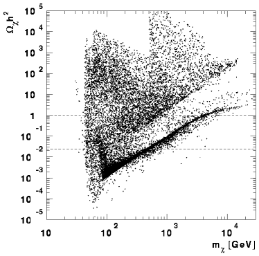
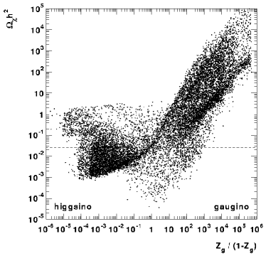
Fig. 4.3 shows the neutralino relic density with coannihilations included versus the neutralino mass and the neutralino composition , respectively. The lower edge on neutralino masses comes essentially from the LEP bound on the chargino mass, Eq. (3.1).
The neutralino is a good dark matter candidate in the cosmologically interesting region limited by the two horizontal lines. There are clearly models with cosmologically interesting relic densities for a wide range of neutralino masses and compositions. The cosmologically interesting region will be discussed more in Section 4.6.5.
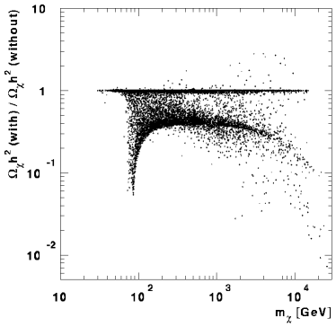
The effect of neutralino and chargino coannihilations on the value of the relic density is summarized in Fig. 4.4, where we plot the ratio of the neutralino relic densities with and without coannihilations versus the neutralino mass and the neutralino composition . In many models, coannihilations reduce the relic density by more than a factor of ten, and in some others they increase it by a small factor. Coannihilations increase the relic density if the effective annihilation cross section . Recalling that is the average of the coannihilation cross sections (see Eq. (4.11)), this occurs when most of the coannihilation cross sections are smaller than and the mass differences of the coannihilating particles are small.
Table 4.2 lists some representative models where coannihilations are important plus one model where coannihilations are negligible. Example 1 contains a light higgsino-like neutralino, example 2 a heavy higgsino-like neutralino. Examples 3 and 4 have , and example 5 has a very pure gaugino-like neutralino. Example 6 is a model with a gaugino-like neutralino for which coannihilations are not important.
| light | heavy | gaugino | ||||
| higgsino | higgsino | bino | ||||
| Example No. | 1 | 2 | 3 | 4 | 5 | 6 |
| [GeV] | 1024.3 | 358.7 | 414.7 | |||
| [GeV] | 3894.1 | 396.6 | ||||
| 1.31 | 40.0 | 2.00 | 7.30 | 37.0 | 22.8 | |
| [GeV] | 656.8 | 737.2 | 577.7 | 828.9 | 2039.5 | 435.1 |
| [GeV] | 610.8 | 1348.3 | 1080.9 | 2237.9 | 4698.0 | 2771.6 |
| 1.97 | ||||||
| 2.75 | 0.52 | |||||
| [GeV] | 76.3 | 1020.8 | 340.2 | 407.8 | 67.2 | 199.5 |
| 0.00160 | 0.00155 | 0.651 | 0.0262 | 0.999968 | 0.99933 | |
| [GeV] | 96.3 | 1026.4 | 364.5 | 418.2 | 133.5 | 396.0 |
| [GeV] | 89.2 | 1023.7 | 362.2 | 414.1 | 133.5 | 396.0 |
| (no coann.) | 0.178 | 0.130 | 0.158 | 0.00522 | 0.418 | |
| 0.0299 | 0.0388 | 0.0890 | 0.00905 | 0.418 | ||
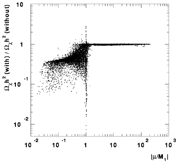
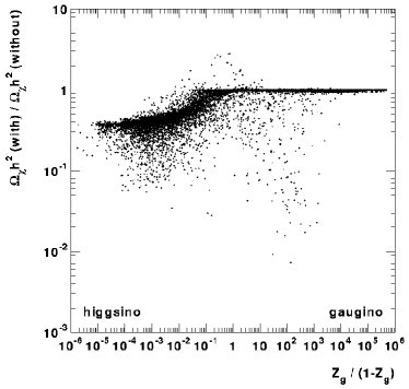
In Fig. 4.5 we show the reduction in relic density due to the inclusion of coannihilations as a function of . A rule of thumb is that coannihilations are important when . But exceptions are found, as can be seen in Fig. 4.5. Notice that when , the neutralino is higgsino-like; when , the neutralino is gaugino-like; and when , the neutralino can be higgsino-like, gaugino-like or mixed.
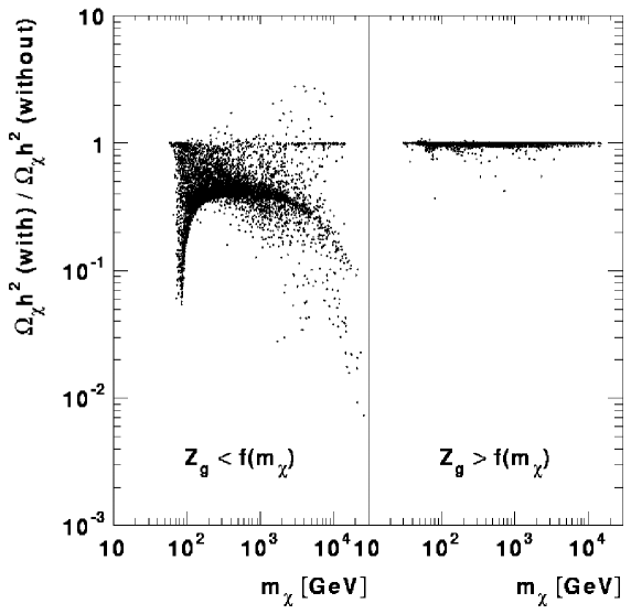
It can be convenient to have a criterium for when coannihilations are important in terms of the composition as well. A rule of thumb is that coannihilations are important when for GeV and when for GeV. There are exceptions to this rule as well, as can be seen in Fig. 4.6 where the ratio of relic densities with and without coannihilations is plotted versus the neutralino mass, the left panel for points satisfying the present criterion, the right panel for those not satisfying it.
In the following subsections, we present the cases where we found that coannihilations are important and explain why. We first discuss the already known case of light higgsino-like neutralinos, continue with heavier higgsino-like neutralinos, the case and finally very pure gaugino-like neutralinos. We then end this section by a discussion of the cosmologically interesting region.
4.6.1 Light higgsino-like neutralinos
We first discuss light higgsino-like neutralinos, , , since coannihilation processes for these have been investigated earlier by other authors [25, 27, 12].
Mizuta and Yamaguchi [25] stressed the great importance of including coannihilations for higgsinos lighter than the boson. For these light higgsinos, neutralino-neutralino annihilation into fermions is strongly suppressed whereas chargino-neutralino and chargino-chargino annihilations into fermions are not. Since the masses of the lightest neutralino and the lightest chargino are of the same order, the relic density is greatly reduced when coannihilations are included. Mizuta and Yamaguchi claim that because of this reduction light higgsinos are cosmologically of no interest.
Drees and Nojiri [27] included coannihilations between the lightest and next-to-lightest neutralino, but did not include those between the lightest neutralino and chargino, which are always more important. In spite of this, they concluded that the relic density of a higgsino-like neutralino will always be uninterestingly small unless GeV or so.
Drees at al. [12] then re-investigated the relic density of light higgsino-like neutralinos. They found that light higgsinos could have relic densities as high as 0.2, and so be cosmologically interesting, provided one-loop corrections to the neutralino masses are included.
We agree with these papers qualitatively, but we reach different conclusions. We show our results in Fig. 4.7, where we plot the relic density of light higgsino-like neutralinos versus their mass with coannihilations included, as well as the ratio between the relic densities with and without coannihilations. The Mizuta and Yamaguchi reduction can be seen in Fig. 4.7b below 100 GeV, but due to the recent LEP2 bound on the chargino mass the effect is not as dramatic as it was for them. If for the sake of comparison we relax the LEP2 bound, the reduction continues down to at lower higgsino masses and we confirm qualitatively the Mizuta and Yamaguchi conclusion — coannihilations are very important for light higgsinos — but we differ from them quantitatively since we find models in which light higgsinos have a cosmologically interesting relic density. For the specific light higgsino models in Drees et al. [12] we agree on the relic density to within 20–30%. We find however other light higgsino-like models with higher , even without including the loop corrections to the neutralino masses.


So there is a window of light higgsino models, GeV, that are cosmologically interesting. All these models have and those with the highest relic densities have . These models escape the LEP2 bound on the chargino mass, GeV, because for the mass of the lightest neutralino can be lower than the mass of the lightest chargino by tens of GeV. By the same token, coannihilation processes are not so important and the relic density in these models remains cosmologically interesting. Most of these models will be probed in the near future when LEP2 runs at higher energies, but some have too large a chargino mass ( GeV) and too large an boson mass ( GeV) to be tested at LEP2. Thus GeV higgsinos with may remain good dark matter candidates even after LEP2.
4.6.2 Heavy higgsino-like neutralinos
Coannihilations for higgsino-like neutralinos heavier than the boson have been mentioned by Drees and Nojiri [27], who argued that they should not change the relic density by much, and by McDonald, Olive and Srednicki [24], who warn that they might change it by an estimated factor of 2. We typically find a decrease by factors of 2–5, and in some models even by a factor of 10 (see the right hand side Fig. 4.7b).
For , the lightest and next-to-lightest neutralinos and the lightest chargino are close in mass, and they annihilate into bosons besides fermion pairs. While the annihilation and coannihilation cross sections into pairs are comparable, the coannihilation of , and into fermion pairs is stronger than the annihilation which is suppressed. This gives the increase in the effective annihilation rate that we observe.
As a result, the smallest and highest masses for which higgsino-like neutralinos heavier than the boson are good dark matter candidates shift up from 300 to 450 GeV and from 3 to 7 TeV respectively.
Together with the result in the previous subsection, we conclude that higgsino-like neutralinos () can be good dark matter candidates for masses in the ranges 60–85 GeV and 450–7000 GeV.
4.6.3 Models with
Coannihilations for mixed or gaugino-like neutralinos have not been included in earlier calculations. It has been believed that they are not very important in these cases. On the contrary, when and there is a very pronounced mass degeneracy among the three lightest neutralinos and the lightest chargino. The ensuing coannihilations can decrease the relic density by up to two orders of magnitude or even increase it by up to a factor of 3. This is easily seen in Fig. 4.5 as the vertical strip at .
If the lightest neutralino is mixed, , coannihilations can increase the relic density, whereas if it is more higgsino-like or gaugino-like they will decrease it. This because the annihilation cross section for mixed neutralinos is generally higher than those for higgsino-like or gaugino-like neutralinos.
The largest decrease we see for this kind of models is when is slightly less than and both are in the TeV region. In this case, the lightest neutralino is a very pure bino, and its annihilation cross section is very suppressed since it couples neither to the nor to the boson. The chargino and other neutralinos close in mass have much higher annihilation cross sections, and thus coannihilations between them greatly reduce the relic density. This big reduction suffices to lower to cosmologically acceptable levels if . This reduction does not occur for masses much lower than a TeV, because the terms in the neutralino mass matrix proportional to the mass prevent such pure bino states and the severe mass degeneracy.
To conclude, when , coannihilations are very important no matter if the neutralino is higgsino-like, mixed or gaugino-like. The relic density can be cosmologically interesting for these models as long as the gaugino fraction : these neutralinos are good dark matter candidates.
4.6.4 Gaugino-like neutralinos with
When , the lightest neutralino is a very pure gaugino. According to the GUT relation Eq. (2.38), the supersymmetric particles next in mass, the next-to-lightest neutralino and the lightest chargino, are twice as heavy. So we expect that coannihilations between them are of no importance.222In models with non-universal gaugino masses, the lightest gaugino-like neutralino can be almost degenerate with the lightest chargino, and coannihilations can be important, as examined e.g. in Ref. [33] In fact, as discussed in section 4.5, coannihilations would need to increase the effective cross section by several orders of magnitude for these large mass differences.
This actually happens in some cases. They show up as the small spread at high in Fig. 4.5. In these models, the lightest neutralino is a very pure bino () and the squarks are heavy. Its annihilation to fermions is suppressed by the heavy squark masses, and its annihilation to and bosons is either kinematically forbidden or extremely suppressed because a pure bino does not couple to and bosons. On the other hand, the lightest chargino annihilates to gauge bosons and fermions very efficiently. The huge increase in the effective cross section, compensated by the large mass difference, reduces the relic density by 10–20%. However, the relic density before introducing coannihilations was of the order of –, and this small reduction is not enough to make these special cases cosmologically interesting.
4.6.5 Cosmologically interesting region


We now summarize when the neutralino is a good dark matter candidate. Fig. 4.8 shows the cosmologically interesting region in the neutralino mass–composition plane versus .
The light higgsino-like region does not extend to the left and down due to the LEP2 bound on the chargino mass. The lower edge in gaugino fraction at is the border of our survey (how high is allowed to be). The upper limit on and the upper limit on the neutralino mass come from the requirement . The hole for higgsino-like neutralinos with masses 85–450 GeV comes from the requirement .
We see that coannihilations change the cosmologically interesting region in the following aspects: the region of light higgsino-like neutralinos is slightly reduced and the big region of heavier higgsinos is shifted to higher masses, the lower boundary shifting from 300 GeV to 450 GeV and the upper boundary from 3 TeV to 7 TeV.
The fuzzy edge at the highest masses is due to models in which the squarks are close in mass to the lightest neutralino, in which case - and -channel squark exchange enhances the annihilation cross section. In these rather accidental cases, coannihilations with squarks are expected to be important and enhance the effective cross section even further. Thus, the upper bound on the neutralino mass of 7 TeV is an underestimate.
Chapter 5 Neutralino Detection by Neutrino Telescopes
As mentioned in Chapter 1, neutralinos can accumulate in the Sun [34, 35, 36] or the Earth [37], annihilate and produce detectable muon neutrinos. In this chapter, the method we have used to predict the muon fluxes resulting from neutralino annihilation in the Sun or Earth will be described. We will also discuss, what signal flux levels that can be probed by neutrino telescopes and what a detected signal will tell us about the neutralino mass.
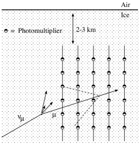
There are many neutrino telescopes in use, e.g. Baksan [38], Macro [39], Kamiokande [40], [41], and others being built and/or proposed, Amanda [42], Nestor [43], and maybe others. A neutrino telescope consists of water or ice situated well below the ground (to minimize the background coming from atmospheric muons). When a neutrino passes by it may interact with the ice or rock surrounding the detector and produce a lepton. If the neutrino is a muon neutrino and hence the lepton a muon, it will neither decay too fast or get stopped too fast and may travel several kilometers (depending on its energy) before getting stopped. As the muon moves through the water (ice) it will emit Čerenkov radiation, which can be detected by photomultipliers. From this signal, the direction of the muon and thus the muon neutrino can be reconstructed. In Fig. 5.1 we show the principle of a neutrino telescope as described above.
In the following sections, the steps performed to obtain a prediction of the muon flux for a given set of MSSM parameters are described. Note however that except for Section 5.3, the results obtained in this chapter are valid for any WIMP and not only neutralinos.
5.1 Neutralino capture and annihilation rates
5.1.1 Capture and annihilation rates
When the Sun and Earth moves through our galactic halo, neutralinos may scatter off nuclei in them and lose enough energy to get gravitationally trapped [34]. They will then oscillate back and forth, occasionally scatter and after a while accumulate in the center of the Sun [35, 36] and the Earth [37] where they can annihilate. The evolution equation for the number of neutralinos, , in the Sun or the Earth is given by
| (5.1) |
where the first term is the neutralino capture, the second term is twice the annihilation rate and the last term is neutralino evaporation. The evaporation term can be neglected for neutralinos heavier than about 5 GeV [44, 45] and since we are not interested in these low-mass neutralinos we can safely drop the last term in Eq. (5.1). If we solve Eq. (5.1) for the annihilation rate we get
| (5.2) |
where is the time scale for capture and annihilation equilibrium to occur. In most cases where the muon fluxes are within reach of present and near-future telescopes, equilibrium will have occurred and the annihilation rate is at ‘full strength’, . Note that in this case, the annihilation rate is determined by the elastic scattering cross sections, on which depends, and not by the annihilation cross section. In our calculation we have of course used the full expressions without assuming that the annihilation occurs at ‘full strength’.
The capture rate depends on, among other things, the local halo mass density, , the velocity dispersion of dark matter particles in the halo, , the elastic scattering cross sections and the composition of the Earth and Sun and we have used the convenient expressions given in Ref. [4] based on the formulas in Ref. [46]. The main uncertainties in the capture rate come from the local halo mass density, , which is uncertain of about a factor of two or so, and the velocity dispersion . We have chosen GeV/cm3 and km s-1. Estimates of can be found in e.g. Ref. [47].
Note that if one-loop corrections to the neutralino coupling to Higgs bosons [12] are included, which we have not, this coupling can for higgsino-like neutralinos either increase by more than two orders of magnitude or in accidental cases be reduced to exactly 0. This means that the spin-independent scattering cross sections for higgsinos can get greatly increased or reduced which mainly effects the capture rate in the Earth (and direct detection experiments which we don’t discuss here). For mixed or gaugino-like neutralinos these one-loop corrections are expected to be small.
5.1.2 Annihilation profiles

The annihilation rate per volume element is given by
| (5.3) |
where is the number density of neutralinos and is the thermally averaged annihilation cross section. The number density of neutralinos is given by [48, 49]
| (5.4) |
with
| (5.5) |
where we in the last step have assumed that the annihilation takes place in the Earth. We have used the Earth radius = 6378 km, the core temperature K and the core density g cm-3. In Fig. 5.2 the resulting projected neutrino angle is shown for neutralino annihilation in the Earth.
For the Sun, the annihilation region is very concentrated to the core and subtends a negligible solid angle as seen from a neutrino telescope at the Earth.
5.2 Muon fluxes - Monte Carlo simulations
A detailed Monte Carlo simulation of the muon fluxes at neutrino telescopes for different annihilation channels and neutralino masses was first done by Ritz and Seckel [50]. We have followed their approach, except for neutrino propagation through the Sun where we have used detailed Monte Carlo simulations [48, 51] instead of the approximate analytical formulae in Ref. [50]. With respect to calculations using Ref. [50] (e.g. Ref. [52]), this Monte Carlo treatment of the neutrino propagation through the Sun increase the muon fluxes by 5–20%.
5.2.1 Annihilation channels and branching ratios
From the previous section we know how to calculate the neutralino annihilation rates and it is straightforward (by e.g. the same methods as described in Section 4.4) to calculate the annihilation branching ratios into different annihilation channels. Since the temperature in both the center of the Earth and Sun is so small, the neutralinos are highly non-relativistic and we can to a good approximation use the zero relative velocity annihilation cross sections to calculate the branching ratios. The annihilation channels of any significance for the muon fluxes are , , , , , , , , , and . Note that the branching ratio into neutrinos directly is zero in the non-relativistic limit and hence the only neutrinos we get are those coming from decay of other annihilation products. We can also not have annihilation into or in this limit since the initial state is CP-odd and so must the final state be. Lighter quarks will not contribute since the annihilation cross section into fermions is approximately proportional to the mass of the fermion squared. Of the charged leptons, only muons and tauons are interesting as potential muon neutrino producers but as we will see in the next subsection, muons will be stopped well before they decay whereas tau leptons do decay before getting stopped so the only lepton channel we have to consider is .
5.2.2 Charged lepton interactions in the Earth
For relativistic charged particles (other than electrons) the mean energy loss is given by the Bethe-Bloch equation [15]
| (5.6) |
where
| (5.7) | |||||
| (5.8) | |||||
| (5.9) |
with being the mass of the particle, its velocity, the atomic number of the stopping material, its atomic weight, its density and the mean excitation energy which is given approximately by
| (5.10) |
At high energies ( 500 GeV for muons in ice), Eq. (5.6) is only a lower limit for the energy loss due to that radiative effects not included in Eq. (5.6) start dominating at high energies. This is however not important in our present analysis, but will be included in Section 5.2.9 where more accurate expressions are needed.
We want to see if muons and tau leptons have time to decay before they get stopped. For muons in the core of the Earth (which consists of mainly liquid iron of density 13.1 g/cm3) the minimum of Eq. (5.6) is
| (5.11) |
from which the mean stopping time is given by . Since the decay time is given by we find that when the ratio
| (5.12) |
is much smaller than one, the particles will get stopped well before they have time to decay. For muons we get
| (5.13) |
and hence any muon produced will be stopped before having time to decay producing any muon neutrinos. For tau leptons, on the other hand, we can in the same way find that the maximal energy loss per second (up to = 5000 GeV) is given by
| (5.14) |
from which it is seen that the upper limit on the energy loss of a tau lepton, is less than a GeV even for TeV energy tauons. Hence energy loss of tau leptons can safely be neglected.
Note that the simple estimates in this subsection could change by a factor of 2–3 or so at high energies, GeV, if radiative effects are included. The conclusion that muons get stopped and that tau lepton interactions can be neglected would be the same though.
5.2.3 Charged lepton interactions in the Sun
For charged lepton interactions in the core of the Sun, which is a plasma, Eq. (5.6) has to be replaced by [53]
| (5.15) |
where is the plasma frequency as given by Eq. (5.9) and is a number of order unity which we put equal to 1. By using that the composition of the core of the Sun is 24% 1H and 64% 4He with a density of 148 g/cm3 [54] we then get the minimal energy loss for muons in the core of the Sun to be
| (5.16) |
and hence
| (5.17) |
Muons are thus stopped well before they decay and can hence be considered as absorbed. For tau leptons we get the maximal energy loss (up to = 5000 GeV) to be
| (5.18) |
which implies that the energy loss is only a few GeV even for TeV tau leptons. Hence tau lepton energy loss can be neglected.
To conclude the previous subsection and this one, muons get stopped well before they decay in both the Earth and Sun and the energy loss of tau leptons can be neglected in both the Earth and Sun.
5.2.4 Heavy hadron interactions in the Sun and Earth
The heavy quarks produced in neutralino annihilation will form mesons and baryons which may interact before they decay. The top quarks will decay before they even have time to form any hadrons and their interactions with the surrounding medium can be neglected. For and quarks however, interactions with the surrounding medium has to be taken care of. This is done in an approximate fashion where the decay/hadronization is simulated as if in vacuum as described below and the interactions that may have occurred are introduced afterwards as a general energy decrease. This approximation is reasonable when the number of interactions is not more than a few which is the case for moderately heavy neutralinos, GeV. For heavier neutralinos neither the nor the channel will dominate and hence the approximation is justified.
The cross sections for and hadron scattering off a nucleon can be estimated by noting that the scattering cross section for any hadron off a proton is approximately given by [55]
| (5.19) |
where is the mean squared strong interaction radius of the hadron. Povh et al. found that fm2, fm2 and fm2. If we assume that the decrease in mean squared radius is constant for each light quark we change to a or quark (justified by experiments) we find that the mean squared strong interaction radii for or mesons and baryons are given by
| (5.20) | |||
| (5.21) |
which together with Eq. (5.19) yields
| (5.22) | |||||
| (5.23) |
From the simulations it is known how far the leading hadron has moved before decaying and the probability that it should have undergone one or more interactions is then easily calculated given the cross sections above. If an interaction is found to have occurred the leading hadron of the new jet takes the energy fraction of the initial hadron. The average energy transfers, , used are those calculated by Ritz and Seckel [50],
| (5.24) | |||||
| (5.25) |
where is the mass of the initial hadron and is the mass of the quark. The same amount of energy decrease is assumed to apply to the produced neutrino. For the channel, interactions are only significant in the Sun and only for heavier neutralinos, GeV. The effect is very dramatic for even more massive neutralinos but for those other annihilation channels will dominate.
5.2.5 Monte Carlo simulations
Of the annihilation channels mentioned above, gauge bosons and tau leptons can decay directly to neutrinos but the quarks will hadronize and eventually give rise to muon neutrinos. The Higgs bosons will decay mainly to quarks which will hadronize as well. All decays and hadronizations are simulated with the Lund Monte Carlo Jetset 7.4 and Pythia 5.7 [56] for each of the annihilation channels , , , , and for the different neutralino masses = 10, 25, 50, 80.2, 91.3, 100, 150, 175, 200, 250, 350, 500, 750, 1000, 3000 and 5000 GeV. Note that the annihilation channels containing Higgs bosons do not need to be simulated separately since the Higgs bosons decay to particles contained in these six ‘fundamental’ channels mentioned above and their contribution to the muon neutrino flux can thus be calculated as soon as the Higgs masses and their decay channels are known. For each mass and annihilation channel, events have been simulated and all muon neutrinos produced have been kept. Hence, a neutrino flux is obtained for any of the given annihilation channels and neutralino masses.
5.2.6 Neutrino interactions and cross sections
The neutrino-nucleon charged and neutral current cross sections are approximately given by
| (5.26) | |||||
| (5.27) |
where the coefficients and are given by
| (5.28) |
| (5.29) |
where GRV structure functions [57] have been used down to . These cross sections agree well with neutrino experiments on isoscalar targets as well as with those obtained using other structure functions, like CTEQ2D [58].
5.2.7 Neutrino interactions in the Sun

Ritz and Seckel [50] considered neutrino interactions on the way out of the Sun in an approximate way where neutral current neutrino-nucleon interactions were assumed to be much weaker than charged current interactions and the energy loss was assumed to be continuous. Neither of these approximations are very good and hence we have instead simulated the neutrino interactions on the way out of the Sun with Pythia 5.7 [56]. For the Earth, the effective thickness is not big enough to be of any importance and neutrino energy loss or absorption on the way to the detector can thus be neglected.
The effective thickness for the Sun is calculated by using the solar model in Ref. [54]. The effective thickness of the Sun is given by of which the part in hydrogen is where is the radius of the Sun. The ’s are given by
| (5.30) | |||||
| (5.31) |
where , is the solar density and is the hydrogen mass fraction. In terms of protons and neutrons the corresponding integrals would be
| (5.32) | |||||
| (5.33) |
With these effective thicknesses and the neutrino-nucleon cross sections, Eqs. (5.26)–(5.29), at hand it is then straightforward to calculate the probability that a given (anti)neutrino has participated in an interaction (charged or neutral current), and if it has (and the interaction is a neutral current interaction) simulate it with Pythia and proceed with the same procedure until the neutrino has reached the surface of the Sun.
In principle one should also take into account the fact that all annihilations don’t occur exactly at the center of the Sun which will introduce a smearing of the effective thickness. This effect can be estimated [48] and is found to be very small. Hence it is a very good approximation to assume that all neutrinos from the Sun originate from the center.
The difference between this approach and the Ritz and Seckel approach is shown in Fig. 5.3 where the neutrino flux weighted by the neutrino energy squared is shown. Note that is approximately proportional to the muon flux since both the neutrino-nucleon cross sections and the muon range are approximately proportional to the energy of the neutrino/muon. The mean energy of the neutrinos at the surface of the Sun is about the same with the Ritz and Seckel approach and this more detailed analysis but the distribution is different and since the muon flux is proportional to the second moment of the distribution (as explained above) one should expect a difference in the predicted muon fluxes at a detector. In fact, the total muon flux with this method is about 5–20% higher than with the Ritz and Seckel approach (with the higher difference at higher masses). Except for this difference in neutrino interactions our results agree well with the Ritz and Seckel results [50] as well as with the analytical results in Ref. [59].
5.2.8 Neutrino interactions at the detector
When a neutrino comes close to the detector it may interact and produce a muon via a charged current interaction. This process is also simulated with Pythia 5.7 [56] where information of not only the muon energy but also the muon angle with respect to the neutrino is kept. For neutralino annihilations in the Earth, the size of the annihilation region has also been included according to the distributions in Eqs. (5.4)–(5.5).
5.2.9 Muon interactions
When a muon is produced it can travel several kilometers (depending on energy) before reaching a detector. When the muons travel through the ice or rock surrounding the detector they may interact and lose energy, where the energy loss is approximately given by
| (5.34) |
where the coefficients and are fitted to the energy losses calculated in Ref. [60] and are given by
| (5.35) |
for muons propagating in water or ice and
| (5.36) |
for muons propagating in rock. The errors of these parameterizations are less than 2% in the region 30–10000 GeV and less than 6% in the region 10–30 GeV. Hence they are sufficiently accurate for our needs. By integrating Eq. (5.34) we get the mean energy of the muons after having traversed a distance of the detector surroundings to be
| (5.37) |
where is the initial muon energy. From this relation we find that the range of a muon of energy is
| (5.38) |
which for low energies, GeV, is approximated by . Note that the radiative effects contained in the -term in Eq. (5.34) are actually stochastic and will lead to energy straggling, i.e. some muons will lose more energy and some less. This is however only important when GeV and for our needs the use of the mean energy as given by Eq. (5.37) is good enough.
The muons will also undergo multiple Coulomb scattering on their way to the detector in which process they don’t lose energy but the angular distribution of the muons gets smeared. For the multiple Coulomb scattering we have used the formulas in Ref. [15].
Since the neutrino flux to a very good approximation is constant in the region surrounding the detector where neutrino-interactions producing detectable muons occur, we for each produced muon choose a distance between 0 and away from the detector where the muon was produced and degrade its energy on its way to the detector according to Eq. (5.37). We also take care of the Multiple Coulomb scattering occurring during this passage of matter as described above.
5.2.10 Resulting muon fluxes
With the methods described above, we have what we need to calculate the muon flux at a detector for a given neutralino (or any WIMP) mass and annihilation channel. As described above, annihilations are simulated for each neutralino mass and annihilation channel. The produced neutrinos are let to interact on their way to the detector and the charged current interactions close to the detector where the muons are produced are simulated. The muons can then interact and scatter on the way to the detector. The (differential) muon flux at the detector is then given by summing up all these muons and weighting each muon by the probability that such a muon would have been created and detected,
| (5.39) |
where is the charged current cross section, Eqs. (5.26) and (5.28), is the number of nucleons per cm3 in the material surrounding the detector, is the range of a muon produced with energy and is the distance from the source (the Sun or the center of the Earth) to the detector.
This way the muon fluxes in units of m-2 annihilation-1 are obtained for the set of masses and annihilation channels given in Section 5.2.5. When a muon flux is needed for another mass, an interpolation is performed and when muon fluxes from other than these ’fundamental’ annihilation channels are needed, e.g. , the flux is easily calculated based on the ’fundamental’ annihilation channels. A Higgs boson will decay in flight to any of the particles for which the muon fluxes are calculated, e.g. . The Higgs bosons are let to decay in flight and the fluxes are obtained by integrating over the production angle of the decay products with respect to the Higgs momentum. The total flux from the Higgs boson is then obtained by summing over all the Higgs decay channels.
In the next section, it is described how the muon fluxes for specific MSSM parameters are obtained.
5.3 Muon fluxes - predictions


We are now ready to apply the results obtained earlier in this chapter and calculate the expected muon fluxes at neutrino telescopes [61]. For other references on predicted rates in neutrino telescopes, see e.g. Ref. [52].
The differential muon flux at a neutrino telescope is given by
| (5.40) |
where is the annihilation rate, Eq. (5.2), is the effective area of the detector in the direction of the source, is the branching ratio for annihilation into annihilation channel and is the differential muon flux from annihilation channel as obtained in the previous section.
In this chapter, we have up till now only assumed that the dark matter candidate we consider is a WIMP, but when we want to make detailed predictions of the muon fluxes at neutrino telescopes we have to specify what WIMP candidate we have, in our case the neutralino. We have performed several different scans of the supersymmetric parameter space as given in Table 2.2 in Section 2.9. For each given model we have checked against all experimental bounds given in Section 3.1 and only kept models not excluded by any experiment.
As soon as the MSSM parameters are chosen, the mass of the neutralino, its composition, the annihilation rate and annihilation branching ratios can be calculated. The annihilation branching ratios in Eq. (5.40) are evaluated with the same methods as those in Section 4.4 but for the relative velocity since the neutralinos are highly non-relativistic when they annihilate in the Earth and Sun.
We are mainly interested in models where the relic density of neutralinos is cosmologically interesting, i.e. , and in the figures shown here (except for Fig. 5.5) we will only show models with a relic density in this desired range. The relic densities are calculated with coannihilations between neutralinos and charginos included as described in Chapter 4.
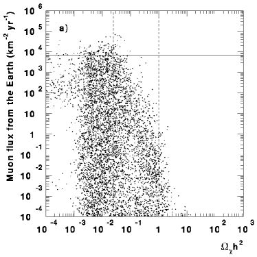
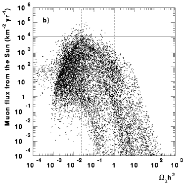
In Fig. 5.4 we show the predicted muon fluxes coming from neutralino annihilation in the Earth and Sun versus neutralino mass. As seen the expected rates in neutrino telescopes vary over several orders of magnitude. The spread is bigger for annihilation in the Earth since the capture rate in the Earth only depends on the spin-independent scattering cross sections whereas the capture rate in the Sun also gets a contribution from the spin-dependent scattering cross sections (due mainly to hydrogen). We also show the limit on the muon fluxes coming from the Baksan experiment [38] and we see that present neutrino telescopes already have started to explore the MSSM parameter space. As will be seen in Section 5.5 an neutrino telescope can explore muon fluxes down to about 50-100 km-2 yr-1 which at least for the Sun is a substantial fraction of the models in Fig. 5.4. Note however that the density of points in these figures does not have any physical meaning, they are just artifacts of how the scanning is performed.
Most of our models with very high muon fluxes (i.e. those probed by Baksan) come from the ’light Higgs’ scan in Table 2.2 where the mass of the boson is low and hence the spin-independent scattering cross sections are high (which means that the capture rates are high).
In Fig. 5.5 we show the expected muon fluxes versus the neutralino relic density. In this figure only we also show models with non-interesting relic densities. For the local halo mass density is rescaled as since for these low relic densities the neutralinos cannot make up all of the galactic halo. The general trend of getting lower muon fluxes for higher is clearly seen. This is due to that the relic density is approximately inversely proportional to the annihilation cross section (see e.g. the approximate expression Eq (1.6)) and due to the crossing symmetry also to the scattering cross section and hence to the annihilation rate. The bend over for is due to the scaling of explained above.
In Fig. 5.6 we show the muon flux from neutralino annihilations in the Earth versus the flux from neutralino annihilations in the Sun. As seen, in most cases the flux from the Sun is higher due to that the capture rate in the Sun also gets contributions from spin-dependent scatterings since there is so much hydrogen in the Sun whereas the capture rate in the Earth only depends on the spin-independent scattering cross sections.
In Fig. 5.7 we compare the muon fluxes in neutrino telescopes with the direct detection rates in 76Ge [21, 61]. Future direct detection experiments may probe event rates down to about 0.01 events kg-1 day-1. We see that for a given factor of improvement in sensitivity, indirect detection from the Sun generally gains more than direct detection which in turn usually gains more than indirect detection from the Earth. Be aware of the huge spread of the points though. Especially in Fig. 5.7b we see a nice complementarity between the two search methods. The reason for this is that spin-dependent scatterings contribute to the flux from the Sun but not to either the flux from the Earth or to the direct detection rates. There are however some direct detection materials which have spin, but the spin-dependent scatterings are even in these cases not contributing much to the direct rates.
We now want to compare these rates in neutrino telescopes with the search potentials of LEP2. LEP2 will mainly put new constraints on the mass of the lightest Higgs boson, , and on the chargino masses. In Fig. 5.8 we show the muon fluxes from neutralino annihilation in the Sun versus the mass. In the upper panel we show models that can be probed by LEP2 after 150 pb-1 of running at 192 GeV [11] and in the lower panel, models not excludable by LEP2 are shown. For the Earth, the corresponding figure would be about the same but with a wider spread of the muon fluxes. Clearly, there is a very nice complementarity between neutrino telescope search capabilities and LEP2 search capabilities. If we are unlucky, however, the Nature has chosen the parameters such that SUSY will escape both neutrino telescopes and LEP2. Note that LEP2 will be able to exclude all our models where GeV.
5.4 Backgrounds
There are a few backgrounds for neutrino telescopes that need to be handled. The largest background is down-going muons produced by cosmic ray particle interactions in the Earth’s atmosphere. These muons don’t survive too far in the Earth though and can thus be reduced by putting the neutrino telescope deep underground. At several kilometers depth there are still a lot of down-going muons present, but since these are down-going and by looking for up-going muons (i.e. when the source is below the horizon) this background does not present a big problem. In the cosmic ray particle interactions in the atmosphere there are however also neutrinos produced [62, 63] and these will constitute the main background since they can not be removed by going deeper underground. By using the atmospheric neutrino fluxes in Ref. [63] and the neutrino to muon conversion formulas in Ref. [64] we find the background muon fluxes underground given in Table 5.1. To obtain these backgrounds we have used the values of and valid for ice, Eq. (5.35), and rock, Eq. (5.36), respectively. We have integrated over a cone of half-aperture angle which in many cases is a reasonable angular width of the signal flux.
| [GeV] | 1 | 10 | 25 | 50 |
|---|---|---|---|---|
| Vertical, ice | 903 | 506 | 359 | 257 |
| Horizontal, ice | 2098 | 1333 | 993 | 742 |
| Vertical, rock | 1030 | 564 | 393 | 275 |
| Horizontal, rock | 2372 | 1474 | 1077 | 788 |
To discriminate the signal from the background one has to use the fact that the signal has an angular (and energy) dependence different from the background as will be discussed in the next section. From the Sun there is also a small background coming from cosmic ray particle interactions in the Sun’s corona [65]. This background will have a similar angular dependence as the signal but a different energy dependence. This background is of the order of 10 events/km2 which is usually below the signals accessible with neutrino telescopes of order 1 km2 being currently planned (see next section). However, in the most sensitive cases where the neutralino mass is high and we have a specific model to test for, this background should be taken into account. Since it will mostly effect the analysis when even bigger neutrino telescopes than (1 km2) are built, we will for the moment neglect this background.
5.5 What signal levels can be probed?
If we now imagine having a specific neutrino telescope, how high must the signal flux be to be detectable? First of all it must be high enough so that we get any events and secondly it must be high enough to be seen above the background. Since the atmospheric background has both a completely different angular and energy distribution than the signal one would expect that it should not be too difficult to observe the signal above this background. In the simplest data analysis one would just look for an excess of events in an angular cone centered around the Earth or Sun with a given half-aperture angle . The angle would be chosen large enough to include as much signal as possible and small enough to exclude as much background as possible. This is what is usually done with neutrino telescopes today. In Ref. [66] was investigated what the optimal would be for different neutralino masses and compositions. Here we go one step further [67] and investigate what could be done if the full angular and/or energy resolution is actually used to discriminate against the atmospheric background. Note, though, that currently designed neutrino telescopes have a very poor energy resolution in the energy region where the signal from neutralino annihilation is.
In the following subsections, we describe how we calculate the expected sensitivities for neutrino detectors with angular and/or energy resolution and present numerical results for some representative models.
5.5.1 ’Single-bin’ analysis
Consider a theory which predicts an upward-muon flux (where the stands for ‘signal’) with an angular distribution , where is the angle the muon makes with the direction of the source of interest, and (i.e. is constant for an isotropic distribution). We would like to disentangle this signal from a background of atmospheric neutrino-induced muons which has a flux with an angular distribution , which is nearly isotropic (at least on small angular scales).
Consider first an experiment that can only tell that a muon has been detected with an angle and an energy , but no further information on the muon direction or energy is available. Then, the angular acceptance cone around the source must be large enough to include all (or most) of the muons produced by neutrinos from the source. One would therefore have some number of muons detected with an angle . For example, in their searches for energetic neutrinos from the Earth and Sun, the Baksan collaboration [38] reports the flux of muons within an angle of the Sun or the center of the Earth. The Kamiokande collaboration [40] reports the flux of muons within an angle varying between –. We will refer to this way of analyzing data as the ‘single-bin’ (or ‘0D’) approach.
With such an experiment, the number of background events after an exposure (for example, in units of km2 yr) is . The number of expected events from the source of interest is . A detection would require an excess of events over the number expected. Then, a excess will be observable only if where .
From such a simple experiment described above where no energy or angular distributions are used, we can conclude that the minimal exposure required for a discovery is
| (5.41) |
where and are the background and signal fluxes above threshold and within the angular cone of acceptance . Note that Eq. (5.41) is only valid when the fluxes are high. This minimal exposure is relevant to the way, e.g., Baksan and Kamiokande have analyzed their data (with different values of ).
In the following more detailed examples, Eq. (5.41) with either or the optimal (which maximizes ) will be used for comparison. Note that for low masses ( GeV) the optimal will be higher than and for high masses it will be lower. However, one cannot know in advance what the optimal cut will be, unless we have a specific model we want to test. If we don’t have a specific model 5∘ is a reasonable choice of giving decent results both for low and high masses. In principle it is however possible to extract the optimal angular cut from data by varying and for the optimal value the signal should be most clearly visible. We have not investigated further how well this method of finding would do, but it will never do better than the single-bin approach where the optimal angular cut is known in advance.
5.5.2 Covariance-matrix analysis
Now consider a slightly more sophisticated experiment which has angular and/or energy resolution. It is possible that we will actually be fitting for both a background and a signal flux of muons where the background flux is given by
| (5.42) |
which we assume to be isotropic (at least over small angular patches), . We will only consider the atmospheric neutrino background resulting from cosmic-ray interactions in the Earth’s atmosphere. In addition, we will want to fit data for an annihilation signal which generally depends on the neutralino (or any WIMP) mass and its composition. We may parameterize this as
| (5.43) |
where parameterizes the relative contributions of a ‘hard’ and ‘soft’ annihilation spectrum. As a ‘hard’ annihilation spectrum we have used the channel below the mass and above and as a ‘soft’ spectrum we have used . These channels represent the extreme hardnesses of the spectrum for any given neutralino mass. For the evaluation of the neutrino and muon flux for these channels we have used the method given earlier in this chapter.
Therefore, we are assuming that the muon angular and/or energy distribution from both background and signal will be described by the set of parameters (one could also envision more parameters). We now want to ask, with what precision can we measure these parameters with a given experiment, assuming the true distribution is given by some set of parameters, ?
To answer this, we assume the data is binned into a number of angle/energy bins, and each bin is centered on angle and energy with widths and . Therefore, for a given set of parameters, the flux will be
| (5.44) |
The probability distribution for the number of events expected in each bin is a Poisson distribution with mean , so it has a width .
So, suppose the true parameters are . Then the probability distribution for observing an angle/energy distribution which is best fit by the parameters is
| (5.45) |
where the curvature matrix is given approximately by
| (5.46) | |||||
where the partial derivatives are evaluated at , and we used in the second line. In a realistic experiment, the width of the bins would be comparable to the angular and/or energy resolution of the experiment. In the limit of perfect angular and energy resolution, the sum becomes an integral,
| (5.47) |
The covariance matrix, gives an estimate of the standard errors that would be obtained from a maximum-likelihood fit to data: The standard error in measuring the parameter (after marginalizing over all the other undetermined parameters) is approximately . If three times the standard error in the parameter is less than , for a given underlying model and for a given experiment, then this model will be distinguishable from background at the level.

If all of the parameters except for are fixed, then is a matrix, i.e. . In this case, Eq. (5.47) reduces to
| (5.48) |
To illustrate, if there were no background, Eq. (5.48) says that the statistical uncertainty in the number of events is the square root of the number of events, and this makes sense. However, if the total number of events is nonzero, then a signal has been discovered.
In fact, if there is no background, and an event is seen, it constitutes discovery. On the other hand, if nothing is seen, the 95% CL upper limit to the number is 3.
5.5.3 Results
We are now ready to perform some actual calculations using the techniques described in the previous subsection for the specific example of neutralino annihilation in the Sun and Earth. We assume that the neutrino energy spectra are either the hard or soft spectra described above; energy spectra from specific neutralino models should fall somewhere between these two extremes. Since the muon flux is proportional to the neutrino energy squared, the hard annihilation channels will generally be more important and hence in general the muon spectra will be more hard than soft. Because of the steep fall with energy of the atmospheric background, hard spectra generally require less exposure. In all integrations with angular (and energy) distribution the integration in Eq. (5.47) is performed up to . For the atmospheric background we have used the results given in Ref. [63].

In Fig. 5.9 the minimal exposures needed to make a discovery are shown for a detector with perfect angular resolution but no energy resolution. The two extreme cases of soft and hard annihilation spectra are shown. In producing Fig. 5.9 we have assumed that only the signal flux parameters in Eq. (5.43) are unknown. This is not unreasonable since the background can be expected to be measured well by an off-source measurement. For annihilation in the Sun the curves are similar but less steep. We find that a neutrino telescope with exposures of about 1–25 km2 yr would be able to detect signal fluxes down to about 50–100 km-2 yr-1.
A comparison with what one could detect if one also has energy resolution is given in Fig. 5.10 where a comparison between how many parameters in Eqs. (5.42) and (5.43) that are known is also shown. We find that by having energy resolution we can gain as much as another factor of two in what signal fluxes we can detect.
In case of a detector with angular resolution but no energy resolution we have also investigated what could be gained by varying the energy threshold and the gain is very small and only for neutralino masses above 100 GeV. Increasing the threshold above 10 GeV gives no further improvements. On the other hand, large detectors (like Amanda) which have a threshold of tens of GeV will not lose much sensitivity either, for neutralino masses above 100 GeV.
5.5.4 Example of a neutrino telescope


Let us now consider a more specific example of a neutrino telescope. We will consider a neutrino telescope with a size of Amanda (at present m2 in the direction of the Earth and m2 in the direction of the Sun) run for 5 years, i.e. with an exposure of km2 yr and km2 yr for the Earth and Sun respectively. In Fig. 5.11 the muon fluxes that can be probed by such a detector is shown. We have here assumed that the muon energy threshold is 25 GeV and that we have an a priori model we want to test, i.e. we have used the optimal angular cut for the ’single-bin’ analysis (0D) and we have only assumed that the signal flux normalization in Eq. (5.43) is unknown for the ‘1D’ case. We show the muon fluxes that can be probed when the neutralino annihilation spectrum is hard. We see that at higher masses it is for Amanda possible to probe fluxes down to a few hundred km-2 yr-1 at high masses.
In Fig. 5.12 we show the muon fluxes that can be probed with a neutrino telescope with an area of 1 km2 run for 10 years, i.e. with an exposure of km2 yr. As above, the optimal angular cut has been used and only is assumed to be unknown. The muon energy threshold has again been assumed to be GeV. We see that such a detector can probe muon fluxes down to about 10 km-2 yr-1 at high masses. In Fig. 5.12b we see that one would gain about a factor of 1.5 by having vertical atmospheric background instead of horizontal. When looking towards the Sun, a neutrino telescope at the poles will have almost horizontal background and a neutrino telescope close to the equator will have horizontal background in the beginning/end of the night and nearly vertical in the middle of the night (how vertical depends on the latitude and season).
In case all three signal flux parameters in Eq. (5.43) are unknown, the curves in Figs. 5.11–5.12 would be about a factor of 1.5–2 higher. If the energy threshold is higher than 25 GeV, the curves will be higher at low masses.
Note that for especially the (1 km2) telescope, as shown in Fig. 5.12, we are in the background dominated regime which means that if we increase the exposure by a given factor, the muon fluxes we can probe decrease by the square root of that factor.


5.5.5 Discussion
We can conclude that if want to test a specific model we only gain about 10–25% by using the full angular resolution compared to the ‘single-bin’ approach. If we don’t have a specific model to test for, which is usually the case, we have to choose an angle in the ‘single-bin’ approach compared to which we can gain up to a factor of 2 by using the angular resolution as proposed here. By using the parameterization of the signal flux, Eq. (5.43) we can also gain some information on the neutralino mass and the hardness of the spectrum though.
By varying the energy threshold not much more is gained, but by having energy resolution about a factor of 1.5–2 can be gained, slightly more at low signal fluxes and slightly less at high signal fluxes.
We also note that for neutrino telescopes with a size of about 1 km2 and only angular reslution, the signal fluxes we can expect to probe is in the region of 50–100 km-2 yr-1 when all three signal parameters in Eq. (5.43) are unkonwn and about a factor of two lower if only the normalization is unkown. If we in addition have energy resolution we gain about a factor of 1.5–2 more. The signal fluxes within reach are almost an order of magnitude larger than the expected background coming from cosmic ray interactions in the Sun (about 10 events km-2 yr-1 [65]). Therefore it is quite safe to neglect this background at the present stage. When detectors are getting even bigger it will however be a severe limitation when looking for the neutrino flux from the Sun since this background is also highly directional as the signal. The energy dependence is quite different though, so having energy resolution may be beneficial in this case.
5.6 What does a detected signal tell?


We have in Eqs. (5.4)–(5.5) and Fig. 5.2 seen that the width of the neutrino distribution depends on the neutralino mass. From Eqs. (5.4)–(5.5) we can derive that the root mean square value of the projected angular distribution given in Fig. 5.2 is
| (5.49) |
If we could measure this width we would, since the width only depends on the neutralino (or any WIMP) mass, be able to determine the neutralino mass in a model-independent fashion. It is however not possible to measure this width directly since we measure the muons and not the neutrinos in neutrino telescopes. When converting the neutrino flux to a muon flux, we will introduce a model dependence, since we need to know the neutrino energy distribution which depends on the branching ratios to different annihilation channels. The angle the muon makes with respect to the neutrino in the charged current scattering decreases as the square root of the neutrino energy, i.e. we will get a smearing of the neutrino distribution which is smaller the harder the annihilation spectrum is and the heavier the neutralino is. The muon will also undergo multiple Coulomb scattering on it way to the detector which further smears the angular distribution. Note that both the intrinsic neutrino angular distribution and the charged current scattering angle tends to widen the angular distributions the lower the neutralino mass is.
As we did in the previous section, we will consider the extreme cases of ‘hard’ and ‘soft’ annihilation spectra where we for the hard spectra use when and when and for the soft spectra we use the annihilation channel. These cases should represent the extreme cases for any neutralino (or any WIMP).
We have calculated the resulting muon angular distributions for hard and soft spectra and for different masses using the methods described earlier in this chapter. In Fig. 5.13 we show the resulting muon distributions for hard annihilation spectra, a muon energy threshold of GeV and a detector (projected) angular resolution of 1.4∘. If we compare Fig. 5.13a with Fig. 5.2 we clearly see the widening of the distributions that the charged current and the multiple Coulomb scatterings give rise to. For neutralino annihilation in the Sun, the neutrino distributions are very narrow peaks at and hence the distributions in Fig. 5.13 reflects the smearing due to the charged current and multiple Coulomb scatterings only.
Using these kind of muon distributions we can now investigate if it is possible to extract the neutralino mass from the width of the muon angular distributions. In Fig. 5.14 we show the neutralino mass versus the full width half maximum of the angular distribution for neutralino annihilation in the Earth. These curves are evaluated for a neutrino telescope with perfect angular resolution. When the resolution is more typical, 1–2∘, the curves bend upwards at the lower-angle end thus reducing the upper limit on the mass for which the mass can be inferred. We find that for neutralino masses GeV, the Earth angular distribution can be used to infer the neutralino mass. If the threshold is low, GeV, the Sun angular distribution can also be used.
If one would observe a signal from both the Earth and Sun, one could imagine subtracting the Sun angular distribution from the Earth one and thus achieve the desired model-independent neutrino angular distribution. This is however not possible to do in a completely model-independent way since the neutrino interactions in the Sun depend on the neutrino spectrum and hence on model parameters. It is probably possible, however, to reduce the model dependence with this technique.
Chapter 6 Conclusions
We have performed a detailed evaluation of the relic density of neutralinos (in the framework of the MSSM) including all two-body final states at tree level and coannihilations between all neutralinos and charginos lighter than . We have found that the neutralino density is cosmologically interesting () for a wide range of neutralino masses and compositions.
The coannihilation processes we have included are important not only for light higgsinos, but whenever , which includes all higgsino-like neutralinos as well as some mixed and gaugino-like neutralinos. In these cases coannihilations can reduce the relic density by typically a factor of 2–5, but sometimes even with up to a factor of 100. We have also found that coannihilations can increase the relic density up to a factor of 3.
There has been claims in the literature [25, 27] that light higgsino-like neutralinos are never cosmologically interesting, but we found, in agreement with Ref. [12], that neutralinos with masses GeV and can be cosmologically interesting.
We have also shown that higgsino-like neutralinos with masses GeV can have and that the upper limit on the neutralino mass for the neutralinos not to overclose the Universe increases from 3 to about 7 TeV when coannihilations are included. It may be noted, though, that massive neutralinos may appear unnatural in the sense that they require fine-tuning of the parameters.
To evaluate the relic density correctly will be even more important in the near future when the cosmological parameters can be expected to be measured quite accurately [68, 69] and we might want to draw some conclusion on the MSSM parameters from such measurements.
We have also evaluated the indirect detection rates in neutrino telescopes coming from neutralino annihilations in the Sun and Earth. The detection rates in neutrino telescopes are found to, for many models, be explorable by the next generation neutrino telescopes, with sizes of especially for neutralino annihilation in the Sun. We have also shown that there is a nice complementarity between which models neutrino telescopes can probe and which can be probed at e.g. LEP2. There are however models giving rise to very small detection rates in neutrino telescopes and that are not explorable by LEP2.
We have also investigated what muon fluxes a given neutrino telescope can probe and we have found that neutrino telescopes with an exposure of about 1–25 km2 yr can probe signal fluxes down to about 50–100 km-2 yr-1 if the full angular distribution of the signal is used. If supersymmetry is found in some other experiment and we know the relevant MSSM parameters, neutrino telescopes of this size will be able to search for such a specific signal down to about 10–50 km-2 yr-1.
We have also shown that if a signal is seen, the width of the angular distribution can be used to infer the neutralino mass. If a signal is seen from the Earth, neutralino masses GeV can be determined. For a signal from the Sun, the mass can be inferred only if the muon energy threshold is small ( 5 GeV).
We can thus at this stage conclude that very exciting times will soon come when the new bigger neutrino telescopes start operating.
Appendix A Feynman Rules for the MSSM
A.1 Introduction
This is a collection of Feynman rules based on the rules given in Ref. [5, 6, 16]. They are slightly rewritten in a format more suitable for numerical implementation and we have used the conventions given in Chapter 2, except for the convention on the matrix that diagonalize the neutralino mass matrix, Eq. (2.10).
In our actual calculations we have used the complex matrix with positive mass eigenvalues as explained in Chapter 2. Another convention is to instead have a real matrix in which case the mass eigenvalues can be either positive or negative. In this convention the neutralinos are instead of Eq. (2.11) given by
| (A.1) |
The relation between the -matrix and the -matrix is [6]
| (A.2) |
where is the sign of the :th mass eigenvalue (i.e. the mass eigenvalues are with ).
The Feynman rules below are given in a form where it is very easy to choose one convention or the other. If the convention with a real matrix is desired, one only has to drop the complex conjugation of whenever that appears and remember that denotes the sign of the :th mass eigenvalue with being the absolute value of the mass eigenvalue. If one instead wants to use the convention with a complex matrix and positive mass eigenvalues (which is the one we have used), one just has to replace by and put all .
In these rules, the elementary charge and hence the electron charge is . Quark charges are given as fractions of and are denoted by , i.e. and .
Where relevant, the vertices are given as where
| (A.3) | |||||
| (A.4) |
are the left- and righthanded projection operators. The indices on the ’s indicate the particles involved, for which we have used the following shorthand notation,
-
any neutralino or chargino.
-
any quark (we only give the rules for one generation, but following Chapter 2 it is straightforward to extend this to three generations),
-
any squark,
-
any Higgs boson,
-
any gauge boson.
Note that the Feynman rules for leptons and sleptons are not given explicitly. They are however easily obtained from the quark and squark Feynman rules by the following substitutions
| (A.5) |
Note that does not exist.
We want to be able to evaluate different diagrams with general vertex couplings and only in the numerical code insert the values of the vertices for the actual particles involved. It is then convenient to have a convention for the order of the indices on the vertices. We have chosen to work with the following convention [71]:
-
•
The first fermion has a bar and is hence outgoing.
-
•
If two Higgses are present, the order of the indices is the order in which they appear in the Lagrangian with the first one complex conjugated. This means for example that for the vertex, is defined as
(A.6) which gives rise to the following Feynman rules
(A.7) or
(A.8) For the charged Higgses, the charge depends on the direction of the momentum of the Higgs. If or is a charged Higgs it is an in the first rule above and an in the second one. For the rules given in the following sections the first Higgs is outgoing and the second one is ingoing and the charges are assigned accordingly.
-
•
If one Higgs boson is present it is complex conjugated, i.e. if it is charged it is an moving out or an moving in.
-
•
If three Higgs bosons are present of which two are charged, the first charged one is complex conjugated.
In the following sections, the Feynman rules for all three-particle vertices are given and in Section A.11 the propagators are given.
A.2 -- vertices
A.2.1
First let us define
| (A.9) | |||||
| (A.10) |
A.2.2
First let us define
| (A.23) | |||||
| (A.24) |
A.2.3
Given the vertex above one can derive [70] the following Feynman rules with changed direction of the arrows
| (A.37) |
| (A.38) |
| (A.39) |
where is the charge conjugation matrix and and are spinor indices explicitly given for the cases of clashing arrows. When working with clashing arrows one should either use the spinor indices explicitly or note that if one writes down the Feynman amplitude according to the direction of the Dirac fermion (the chargino), the vertices with clashing arrows will appear as given above and if the direction is instead chosen as the one given by the neutralino the vertices will appear transposed.
A.3 -- vertices
A.3.1
First let us define
| (A.40) | |||||
| (A.41) |
A.3.2
First let us define
| (A.48) | |||||
| (A.49) |
A.3.3
A.3.4
A.4 -- vertices
Note that if we have the vertex
| (A.60) |
then it follows [70] that the vertex with reversed arrows is given by
| (A.61) |
A.4.1
A.4.2
First let us define
| (A.80) | |||||
| (A.81) | |||||
| (A.82) | |||||
| (A.83) |
A.5 -- vertices
A.5.1
These vertices can be written [6, Fig. 7 and 8]
| (A.99) |
where
| (A.100) | |||||
| (A.101) | |||||
| (A.102) | |||||
| (A.103) | |||||
| (A.104) | |||||
| (A.105) |
A.5.2
A.5.3
A.6 -- vertices
These vertices can be written [5, Fig. 71]
| (A.113) |
where
| (A.114) | |||||
| (A.115) | |||||
| (A.116) | |||||
| (A.117) | |||||
| (A.118) | |||||
| (A.119) | |||||
| (A.120) | |||||
| (A.121) | |||||
| (A.122) |
A.7 -scalar-scalar vertices
A.7.1
These vertices can all be written [6, Fig. 9 and 10]
| (A.123) |
where
| (A.124) | |||||
| (A.125) | |||||
| (A.126) | |||||
| (A.127) | |||||
| (A.128) | |||||
| (A.129) | |||||
| (A.130) | |||||
| (A.131) |
A.7.2
These vertices can all be written [6, Fig. 11–14]
| (A.132) |
where
| (A.133) | |||||
| (A.134) | |||||
| (A.135) | |||||
| (A.136) | |||||
| (A.137) | |||||
| (A.138) | |||||
| (A.139) | |||||
| (A.140) | |||||
| (A.141) | |||||
| (A.142) | |||||
| (A.143) | |||||
| (A.144) | |||||
| (A.145) | |||||
| (A.146) | |||||
| (A.147) | |||||
| (A.148) | |||||
| (A.149) | |||||
| (A.150) | |||||
| (A.151) | |||||
| (A.152) |
A.8 -scalar-scalar vertices
A.8.1
These vertices can all be written [6, Fig. 1 and 2]
| (A.154) |
where
| (A.155) | |||||
| (A.156) | |||||
| (A.157) | |||||
| (A.158) | |||||
| (A.159) | |||||
| (A.160) | |||||
| (A.161) | |||||
| (A.162) | |||||
| (A.163) | |||||
| (A.164) |
A.8.2
These vertices can all be written [5, Fig. 72]
| (A.165) |
where
| (A.166) | |||||
| (A.167) | |||||
| (A.168) | |||||
| (A.169) | |||||
| (A.170) | |||||
| (A.171) | |||||
| (A.172) |
A.9 -- vertices
A.10 -- vertices
A.11 Propagators
First define the Mandelstam variables
| (A.182) | |||||
| (A.183) | |||||
| (A.184) |
We then have the following propagators [16] for internal particles
| Internal scalar: | (A.185) | ||||
| Internal gauge boson: | (A.186) | ||||
| Internal fermion: | (A.187) | ||||
where as usual with being the width of the propagating particle and its mass. The fermion propagator can in the -channel be written
| (A.188) |
where
| (A.189) |
and in the -channel be written
| (A.190) |
where
| (A.191) |
The -diagram can, when the incoming particles are Majorana fermions (like the neutralinos), be written in the convenient form
| (A.192) |
Summary of the Papers
-
I.
The whole chain of processes from the neutralino annihilation products in the core of the Sun or Earth to a muon flux at a detector is calculated with Monte Carlo simulation techniques.
-
II.
If a positive signal of WIMP annihilations in the Sun or Earth is seen at a neutrino telescope, it is here shown that the mass of the WIMP can be inferred from the width of the angular distribution.
-
III.
The indirect detection rates at neutrino telescopes for neutralino annihilation in the Sun or Earth are evaluated and also compared with direct neutralino dark matter searches and searches at LEP2.
-
IV.
The minimal exposures needed to make a discovery of WIMP annihilations in the Sun or Earth are calculated for different WIMP masses, compositions and signal fluxes.
-
V.
The relic density of neutralinos is calculated including so called coannihilation processes between the lightest neutralino and heavier neutralinos and charginos.
Acknowledgments
First of all I would like to thank my supervisor Héctor Rubinstein for his great support and my assistant supervisor Lars Bergström who has been most helpful during my studies and for his careful reading of the manuscript.
I would also like to thank Paolo Gondolo for the many valuable discussions we have had, for teaching me the helicity amplitude method for calculating cross sections and for letting me use and develop the programs he has written.
I also want to thank Gunnar Ingelman for interesting discussions in the very early stages of this work. My thanks also go to Anders Edin and Mats Thunman for the discussions we have had.
My colleagues and the personnel at the Department of Theoretical Physics also deserve to be thanked for making my studies more pleasant and interesting.
I would also like to thank my dog, Molly, for not letting me write on my thesis too much by requiring frequent walks and for her deep insight that she is the most important dark matter in the Universe (she is a black Labrador Retriever).
Finally, my warmest thanks go to my wife, Lisa, for her love and support and, not to forget, help with the frequent walks with our dog Molly.
Bibliography
- [1] M. Strauss and J. Willick, Phys. Rep. 261 (1995) 271; A. Dekel, Ann. Rev. Astron. Astrophys. 32 (1994) 319.
- [2] E.W. Kolb and M.S. Turner, The Early Universe, Addison-Wesley (1990).
- [3] See e.g. C. Copi, D.N. Schramm and M.S. Turner, Science 267 (1995) 192, Phys. Rev. Lett. 75 (1995) 3981; N. Hata et al., Phys. Rev. Lett. 75 (1995) 3977.
- [4] G. Jungman, M. Kamionkowski and K. Griest, Phys. Rep. 267 (1996) 195.
- [5] H.E. Haber and G.L. Kane, Phys. Rep. 117 (1985) 75.
- [6] J.F. Gunion and H.E. Haber, Nucl. Phys. B272 (1986) 1 [Erratum-ibid. B402 (1993) 567].
- [7] J. Wess and J. Bagger, Supersymmetry and Supergravity, 2nd Ed. (Princeton University Press, Princeton, 1992).
- [8] J.F. Gunion, H.E. Haber, G. Kane and S. Dawson, The Higgs Hunter’s Guide, Addison-Wesley (1990).
- [9] M. Carena, J.R. Espinosa, M. Quirós and C.E.M. Wagner, Phys. Lett. B355 (1995) 209.
- [10] M. Berger, Phys. Rev. D41 (1990) 225; H.E. Haber and R. Hempfling, Phys. Rev. Lett. 66 (1991) 1815; P.H. Chankowski, S. Pokorski and J. Rosiek, Phys. Lett. B281 (1992) 100; J. Ellis, G. Ridolfi and F. Zwirner, Phys. Lett. B257 (1991) 83; Y. Okada, M. Yamaguchi and T. Yanagida, Phys. Lett. B262 (1991) 54; A. Brignole, Phys. Lett. B281 (1992) 284; J. Kodaira, Y. Yasui and K. Sasaki, Phys. Rev. D50 (1994) 7035.
- [11] E. Accomando et al., Higgs Physics at LEP2, hep-ph/9602250, to appear in Vol. 1, Report of the Workshop on Physics at LEP2, G. Altarelli, T. Sjöstrand and F. Zwirner (eds), CERN 96-01.
- [12] M. Drees, M.M. Nojiri, D.P. Roy and Y. Yamada, hep-ph/9701219.
- [13] D. Pierce and A. Papadopoulos, Phys. Rev. D50 (1994) 565, Nucl. Phys. B430 (1994) 278; A.B. Lahanas, K. Tamvakis and N.D. Tracas, Phys. Lett. B324 (1994) 387.
- [14] M. Drees, K. Hagiwara and A. Yamada, Phys. Rev. D45 (1992) 1725.
- [15] R.M. Barnett et al (Particle Data Group), Phys. Rev. D54 (1996) 1.
- [16] F. Mandl and G. Shaw, Quantum Field Theory, John Wiley & Sons, 1984.
- [17] See e.g. A.S. Belyaev and A.V. Gladyshev, hep-ph/9703251.
- [18] G. Cowan (ALEPH Collaboration), talk presented at the special CERN particle physics results from the LEP run at 172 GeV, 25 February 1997.
- [19] M.S. Alam et al. (CLEO Collaboration), Phys. Rev. Lett. 71 (1993) 674; Phys. Rev. Lett. 74 (1995) 2885.
- [20] S. Bertolino, F. Borzumati, A. Masiero and G. Ridolfi, Nucl. Phys. B353 (1991) 591.
- [21] L. Bergström and P. Gondolo, Astropart. Phys. 5 (1996) 263.
- [22] K. Griest and D. Seckel, Phys. Rev. D43 (1991) 3191.
- [23] Some selected references are: H. Goldberg, Phys. Rev. Lett. 50 (1983) 1419; L.M. Krauss, Nucl. Phys. B227 (1983) 556; J. Ellis et al., Nucl. Phys. B238 (1984) 453; K. Griest, Phys. Rev. D38 (1088) 2357 [erratum ibid D39 (1989) 3802]; J. Scherrer and M.S. Turner, Phys. Rev. D33 (1986) 1585 [erratum ibid D34 (1986) 3263]; K.A. Olive and M. Srednicki, Phys. Lett. B230 (1989) 78, Nucl. Phys. B355 (1991) 208; K. Griest, M. Kamionkowski and M.S. Turner, Phys. Rev. D41 (1990) 3565; G.B. Gelmini, P. Gondolo, and E. Roulet, Nucl. Phys. B351 (1991) 623; A. Bottino, V. de Alfaro, N. Fornengo, G. Mignola and S. Scopel, Astropart. Phys. 1 (1992) 61; A. Bottino, V. de Alfaro, N. Fornengo, G. Mignola, M. Pignone, Astropart. Phys. 2 (1994) 67; H. Baer and M. Brhlik, Phys. Rev. D53 (1996) 597. For further references, see G. Jungman, M. Kamionkowski, and K. Griest, Phys. Rep. 267 (1996) 195.
- [24] J. McDonald, K.A. Olive and M. Srednicki, Phys. Lett. B283 (1992) 80.
- [25] S. Mizuta and M. Yamaguchi, Phys. Lett. B298 (1993) 120.
- [26] M. Srednicki, R. Watkins and K.A. Olive, Nucl. Phys. B310 (1988) 693.
- [27] M. Drees and M. Nojiri, Phys. Rev. D 47 (1993) 376.
- [28] P. Gondolo and G. Gelmini, Nucl. Phys. B360 (1991) 145.
- [29] J. Edsjö and P. Gondolo, hep-ph/9704361, submitted to Phys. Rev. D.
- [30] P. Gondolo and J. Edsjö, in preparation.
- [31] Reduce 3.5. A.C. Hearn, RAND, 1993.
- [32] P. Gondolo, in preparation.
- [33] C.H. Chen, M. Drees, and J.F. Gunion, Phys. Rev. D55 (1997) 330.
- [34] W.H. Press and D.N. Spergel, Astrophys. J. 296 (1985) 679.
- [35] J. Silk, K. Olive, and M. Srednicki, Phys. Rev. Lett. 55 (1985) 257.
- [36] L.M. Krauss, K. Freese, D.N. Spergel and W.H. Press, Astrophys. J. 299 (1985) 1001; T. Gaisser, G. Steigman and S. Tilav, Phys. Rev. D34 (1986) 2206; B.A. Campbell, J. Ellis, K. Enqvist, D.V. Nanopoulos, J. Hagelin and K.A. Olive, Phys. Lett. B173 (1986) 270; M. Srednicki, K. Olive and J. Silk, Nucl. Phys. B279 (1987) 804; K. Griest and D. Seckel, Nucl. Phys. B283 (1987) 681; J. Hagelin, K. Ng and K. Olive, Phys. Lett. B180 (1987) 375; K. Ng, K.A. Olive and M. Srednicki, Phys. Lett. B188 (1987) 138.
- [37] K. Freese, Phys. Lett. B167 (1986) 295; L. Krauss, M. Srednicki and F. Wilczek, Phys. Rev. D33 (1986) 2079; T. Gaisser, G. Steigman and S. Tilav, Phys. Rev. D34 (1986) 2206.
- [38] M.M. Boliev et al., Bull. Acad. Sci. USSR, Phys. Ser. 55 (1991) 126 [Izv. Akad. Nauk. SSSR, Fiz. 55 (1991) 748]; M.M. Boliev et al., in TAUP 95, proceedings of the Workshop, Toledo, Spain, September 17–21, 1995, edited by A. Morales, J. Morales and J.A. Villar, [Nucl. Phys. (Proc. Suppl.) B48 (1996) 83] (North-Holland, Amsterdam, 1996).
- [39] E. Diehl, Ph.D. Thesis, U. of Michigan (1994).
- [40] M. Mori et al. (Kamiokande Collaboration), Phys. Lett. B289 (1992) 463; M. Mori et al. (Kamiokande Collaboration), Phys. Rev. D48 (1993) 5505.
- [41] Y. Totsuka, in TAUP 95, proceedings of the Workshop, Toledo, Spain, September 17–21, 1995, edited by A. Morales, J. Morales and J.A. Villar, [Nucl. Phys. (Proc. Suppl.) B48 (1996) 547].
- [42] P.O. Hulth et al (AMANDA Collaboration), to be published in Proceedings of the XVII International Conference in Neutrino Physics and Astrophysics, Neutrino 96, Helsinki, Finland 13-19 June 1996, eds. K. Enqvist, K. Huitu and J. Maalampi (World Scientific, Singapore, 1997).
- [43] L. Resvanis, Europhys. News 23 (1992) 172.
- [44] K. Griest and D. Seckel, Nucl. Phys. B283 (1987) 681.
- [45] A. Gould, Astrophys. J. 321 (1987) 560.
- [46] A. Gould, Astrophys. J. 321 (1987) 571; ibidem 368 (1991) 610; ibidem 388 (1992) 338.
- [47] J.N. Bahcall, M. Schmidt and R.M. Soneira, Astrophys. J. 265 (1983) 730; J.A.R. Caldwell and J.P. Ostriker, Astrophys. J. 251 (1981) 61; M.S. Turner, Phys. Rev. D33 (1986) 889; R.A. Flores, Phys. Lett. B215 (1988) 73; E.I. Gates, G. Gyuk and M.S. Turner, Astrophys. J. Lett. 449 (1995) L123.
- [48] J. Edsjö, Neutrino-induced Muon Fluxes from Neutralino Annihilations in the Sun and in the Earth, Diploma Thesis, TSL/ISV-93-0091, ISSN 0284-2769.
- [49] J. Edsjö and P. Gondolo, Phys. Lett. B357 (1995) 595.
- [50] S. Ritz and D. Seckel, Nucl. Phys. B304 (1988) 877.
- [51] J. Edsjö, Nucl. Phys. B (Proc. Suppl.) 43 (1995) 265.
- [52] G.F. Giudice and E. Roulet, Nucl. Phys. B316 (1989) 429; F. Halzen, T. Stelzer and M. Kamionkowski, Phys. Rev. D45 (1992) 4439; M. Drees, G. Jungman, M. Kamionkowski and M.M. Nojiri, Phys. Rev. D49 (1994) 636; R. Gandhi, J.L. Lopez, D.V. Nanopoulos, K. Yuan and A. Zichichi, Phys. Rev. D49 (1994) 3691; A. Bottino, N. Fornengo, G. Mignola and L. Moscoso, Astropart. Phys. 3 (1995) 65; G. Jungman and M. Kamionkowski, Phys. Rev. D51 (1995) 328; V. Berezinsky, A. Bottino, J. Ellis, N. Fornengo, G. Mignola and S. Scopel, Astropart. Phys. 5 (1996) 333.
- [53] J.D. Jackson, Classical Electrodynamics, 2nd Ed., John Wiley & Sons (1975).
- [54] J.N. Bahcall and R.K. Ulrich, Rev. Mod. Phys. 60 (1988) 297.
- [55] B. Povh and J. Hüfner, Phys. Lett. B245 (1990) 653.
- [56] T. Sjöstrand, Comp. Phys. Comm. 82 (1994) 74; T. Sjöstrand, PYTHIA 5.7 and JETSET 7.4. Physics and Manual, CERN-TH.7112/93, hep-ph/9508391 (revised version).
- [57] M. Glück, E. Reya and A. Vogt, Z. Phys. C53 (1992) 127.
- [58] J. Botts et al., Phys. Lett. B304 (1993) 159.
- [59] G. Jungman and M. Kamionkowski, Phys. Rev. D51 (1995) 328.
- [60] W. Lohmann, R. Kopp and R. Voss, Energy loss of muons in the energy range 1–10000 GeV, CERN Report 85-03 (1985).
- [61] L. Bergström, J. Edsjö and P. Gondolo, Phys. Rev. D55 (1997) 1765.
- [62] L.V. Volkova, Yad. Fiz. 31 (1980) 1510 [Sov. J. Nucl. Phys. 31 (1980) 784]; T.K. Gaisser, T. Stanev and G. Barr, Phys. Rev. D38 (1988) 85; G. Barr, T.K. Gaisser and T. Stanev, Phys. Rev. D39 (1989) 3532; P. Lipari, Astropart. Phys. 1 (1993) 195. M. Thunman, G. Ingelman and P. Gondolo, AStrop. Phys. 5 (1996) 309.
- [63] M. Honda et al., Phys. Rev. D52 (1995) 4985.
- [64] T.K. Gaisser and T. Stanev, Phys. Rev. D30 (1984) 985.
- [65] D. Seckel, T. Stanev and T.K. Gaisser, Astrophys. J. 382 (1991) 652; G. Ingelman and M. Thunman, Phys. Rev. D54 (1996) 4385.
- [66] A. Bottino, N. Fornengo, G. Mignola and L. Moscoso, Astropart. Phys. 3 (1995) 65.
- [67] L. Bergström, J. Edsjö and M. Kamionkowski, astro-ph/9702037, Astrop. Phys., in press.
- [68] R.J. Bond, R. Crittenden, R.L. Davis, G. Efstathiou and P.J. Steinhardt, Phys. Rev. Lett. 72 (1994) 13; G. Jungman, M. Kamionkowski, A. Kosowsky and D.N. Spergel, Phys. Rev. Lett. 76 (1996) 1007, Phys. Rev. D54 (1996) 1332; J.R. Bond, G. Efstathiou and M. Tegmark, astro-ph/9702100.
- [69] C. Bennett et al., MAP home page, http://map.gsfc.nasa.gov/; M. Bersanelli et al., ESA Report D/SCI(96)3, PLANCK home page, http://astro.estec.esa.nl/SA-general/Projects/Cobras/cobras.html
- [70] Derived from the rules in Fig. 83 in Ref. [5] or directly from the Lagrangian.
- [71] P. Gondolo, private communication.