LU TP 97-07

April 1997

Bose-Einstein Correlations in the Lund Model
Bo Andersson and Markus Ringnér

Department of Theoretical Physics, Lund University,

Sölvegatan 14A, S-223 62 Lund, Sweden

Abstract:
By providing the Lund Model fragmentation process with a quantum-mechanical framework we extend the results of [6] to situations where there are very many identical bosons. We investigate the features of the weight distributions in some detail and in particular exhibit three-particle BE-correlations, the influence on the $\rho$-spectrum and the difference between charged and neutral pion correlations.

PACS codes: 12.38Aw, 13.85, 13.87Fh

Keywords: Bose-Einstein Correlations, Fragmentation, The Lund Model, QCD

1 Introduction

The Hanbury-Brown-Twiss (HBT) effect [1] originated in astronomy where one uses the interference pattern of the photons to learn about the size of the photon emission region, i.e. the size of the particular star, which is emitting the light. The effect can be described as an enhancement of the two-particle correlation function that occur when the two particles are identical bosons and have very similar energy-momenta. A well-known formula [2] to relate the two-particle correlation function (in four-momenta $p_{j},j=1,2$ with $q=p_{1}-p_{2}$) to the space–time density distribution, $\rho$, of (chaotic) emission sources is,

$$\frac{\sigma d\sigma_{12}}{d\sigma_{1}d\sigma_{2}}=1+|{\cal R}(q)|^{2}$$ (1)

where ${\cal R}$ is the normalised Fourier transform of the source density

$${\cal R}(q)=\frac{\int\rho(x)dx\exp(iqx)}{\int\rho(x)dx}$$ (2)

This quantity is often, without very convincing reasons, parametrised in terms of a “source radius” $R$ and a “chaoticity parameter” $\lambda$,

$${\cal R}(q)=\lambda\exp(-R^{2}Q^{2})$$ (3)

with $Q^{2}=-q^{2}$. The source radii obtained by this parametrisation tend to be similar in all hadronic interations (we exclude heavy ion interactions where the extensions of nuclear targets and probes will influence the result), with $R\sim 0.5-1~{}fm$, but the chaoticity varies rather much depending upon the particular data sample and the method of the fit. At present the knowledge of higher-order correlations is still limited in the experimental data, although in principle there should be such correlations.

The HBT effect, being of an intrinsically quantum mechanical nature, is not easily included in the event generator programs used in high energy physics. Such simulation programs, like HERWIG [3] (based upon the Webber–Marchesini parton cascades and ending by cluster fragmentation) and JETSET [4] (based upon the Lund Model string dynamics [7]) are built in accordance with classical stochastical processes, i.e. they produce a probability weight for an event without any quantum mechanical interference effects.

Sjöstrand has introduced a clever device as a subroutine to JETSET, in which the HBT effect is simulated as a mean field potential attraction between identical bosons [5]. Thus, given a set of energy-momentum vectors of identical bosons, $p_{1},\ldots,p_{n}$, generated without any HBT effect, it is possible to reshuffle the set into another set where each pair on the average has been moved relatively closer to show a (chosen) HBT-correlation, while still keeping to energy-momentum conservation for the whole event.

In this paper we will develop a method deviced in [6] to provide the Lund Model with a quantum mechanical interpretation. In particular there will be a production matrix element with well-defined phases. This will then be used to make a model of the HBT effect. Although this model stems from different considerations it will nevertheless contain predictions which are similar to those in the ordinary approach giving Eq (1).

In the first section we survey those features of the Lund model, that are necessary for the following. In the second section we will exhibit the general $n$-particle HBT-correlations in the model. The resulting expressions contain a sum of in general $n!$ terms, i.e. it is of exponential type from a computational point of view. It is possible to subdivide the expressions in accordance with the group structure of the permutation group. Although the higher order terms provide small contributions in general the computing times are still forbidding. In order to speed up the calculations we introduce instead the notion of links between the particles and it is in this way possible to obtain expressions of power type from a calculational point of view, which are perfectly tractable in a computer. In the last section we exhibit a set of results both in order to show the workings of the model and to provide predictions for experiments.

We will in this paper be satisfied to treat only two-jet events, i.e. we will neglect hard gluon radiation and we will come back to HBT effects in gluon events in another publication.

2 Some Properties of the Lund Model

Within the framework of perturbative QCD it is possible to obtain many useful formulas but all the results are expressed in a partonic language. In order to be able to compare to the hadronic distributions, which are observed in the experimental setups, it is necessary to supplement the perturbative results with a fragmentation process. We will in this paper be concerned with the Lund string model [7] and we start with a brief introduction to its main properties.

In the string model the confining colour field is approximated by a massless relativistic string. The endpoints of the string are identified with quark and antiquark properties while the gluons are assumed to behave as transverse excitations on the string. The string can break up into smaller pieces by the production of $q\bar{q}$-pairs (i.e. new endpoints). Such a pair will immediately start to separate because of the string tension, which in the rest frame of a string segment corresponds to a constant force $\kappa$; phenomenologically $\kappa\simeq 1$ $GeV/fm$. Final state mesons are formed from a $q$ and a $\bar{q}$ from adjacent vertices, as shown in Fig 1.

Each breakup vertex will separate the string into two causally disconnected parts. From the causality, together with Lorentz covariance and straightforward kinematics, it is possible to derive a unique breakup rule for the string by means of (semi)classical arguments [8].

The unique breakup rule results in the following probability for a string to decay into hadrons $(p_{1},\dots,p_{n})$.

$$dP(p_{1},...,p_{n})=\left[\prod_{i}(Ndp_{i}\delta(p_{i}^{2}-m_{i}^{2}))\right]\delta(\sum_{j}p_{j}-P_{tot})\exp(-bA)$$ (4)

where A is the area of the breakup region as indicated in Fig 1 and N and b are two parameters.

The similarity of the result to Fermi’s Golden Rule for the probability of a quantum mechanical transition, i.e. the size of the final state phase space multiplied by the square of a matrix element $|{\cal M}|^{2}$ expressed by the exponential area suppression, provides a reasonable starting point to try to derive a corresponding quantum mechanical process. There is at least two possible mechanisms, viz. a quantum mechanical tunneling process a la Schwinger and/or the possible relationship to the Wilson loop operators in a gauge field theory. We will find that they provide very similar answers to the problem.

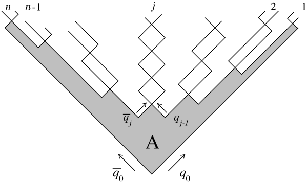
Figure 1: The decay of a Lund Model string.

Starting with the tunneling arguments, we note that while a massless $q\bar{q}$-pair without transverse momentum can be produced in a pointlike way anywhere along the string, a massive pair or a pair with transverse momentum must classically be produced at a distance so that the string energy between them can be used to fulfil energy-momentum conservation. If the transverse momentum is conserved in the production process, i.e. the $q\bar{q}$ with masses $\mu$ obtain $\pm\vec{k}_{\perp}$, respectively, then the pair may classically be realised at a distance $\delta x=2\mu_{\perp}/\kappa$, where $\mu_{\perp}$ is the transverse mass $\sqrt{\mu^{2}+\vec{k}_{\perp}^{2}}$.

The probability for a quantum mechanical fluctuation of a pair, occurring with $\mu_{\perp}$ at the (space-like) distance $\delta x$, is in a force-free region given by the free Feynman propagator squared:

$$|\Delta_{F}(\delta x,\mu_{\perp})|^{2}\sim\exp(-2\mu_{\perp}\delta x)=\exp\left(-\frac{4\mu_{\perp}^{2}}{\kappa}\right)$$ (5)

A corresponding quantum mechanical tunneling process in a constant force field will according to WKB methods give

$$\left|\exp\left(-2\int_{0}^{\delta x}\sqrt{\mu_{\perp}^{2}-(\kappa x)^{2}}dx\right)\right|^{2}=\exp\left(-\frac{\pi\mu_{\perp}^{2}}{\kappa}\right)\equiv P(\mu_{\perp})$$ (6)

The difference is that in the force-free case we obtain an exponential suppression $4\mu_{\perp}^{2}/\kappa$ but when the constant force pulls the pair apart we obtain the somewhat smaller suppression $\pi\mu_{\perp}^{2}/\kappa$. Besides the mass suppression (which phenomenologically will suppress strange quark-pairs with a factor of $\sim 0.3$ compared to “massless” up and down flavored pairs) we obtain the transverse momentum Gaussian suppression

$$\exp\left({-\frac{1}{2\sigma^{2}}k_{\perp}^{2}}\right)~{}~{}\mbox{with}~{}~{}2\sigma^{2}=\frac{\kappa}{\pi}$$ (7)

The value of $\sigma$ as used in JETSET is a bit larger than the result in Eq (7) but this can be understood as an effect of soft gluon generation along the string. The transverse momentum of a hadron produced in the Lund Model is then the sum of the transverse momenta of its constituents.

We may use the elementary result in Eq (6) to calculate the persistence probability of the vacuum, ${\cal P}$, as it is defined in [9]. It is the probability that the no-particle vacuum will not break up, owing to pair-production, during the time $T$ over a transverse region $A_{\perp}$, when a constant force $\kappa$ is applied along the longitudinal x-direction over a region $L$:

$${\cal P}=\prod_{t\in(0,T),x\in(0,L),\vec{k}_{\perp},s,f}(1-P(\mu_{\perp}))=\exp\left(\sum_{t,x,\vec{k}_{\perp},s,f}\log(1-P)\right)$$ (8)

We have then assumed that the field couples to (fermion) pairs with spin $s$ and flavors $f$ and we sum over all possibilities for the production. As each pair needs a longitudinal size $\delta x=2\mu_{\perp}/\kappa$ and, according to Heisenberg’s indeterminacy relation, will live during a timespan $2\pi/2\mu_{\perp}$ there is at most $\kappa LT/2\pi$ pairs possible over the space-time region $LT$. The transverse momentum summation can be done by Gaussian integrals from an expansion of $\log(1-P)$ and the introduction of the well-known number of waves available in a transverse region $A_{\perp}$: $(A_{\perp}/(2\pi)^{2})d^{2}k_{\perp}$. In this way we obtain for the persistence probability

$${\cal P}=\exp(-\kappa^{2}LTA_{\perp}\Pi)~{}~{}~{}\mbox{with}~{}~{}~{}\Pi=\frac{n_{f}n_{s}}{4\pi^{3}}\sum_{n=1}^{\infty}\frac{1}{n^{2}}\exp\left(-\frac{n\pi\mu^{2}}{\kappa}\right)$$ (9)

where $n_{f},n_{s}$ is the number of flavor and spin states.

There are two remarks to this result. Firstly, although the method to treat the integration over time and longitudinal space, by close-packing reasonably sized boxes, may not seem convincing the final formula [9] coincides with the one obtained by Schwinger [10], for the case of a constant electric field ${\cal E}$. Then $\kappa$ is identified with the force of the charges in the external field, i.e. $\kappa\rightarrow e{\cal E}$.

Secondly, the result is in evident agreement with the formula for the decay of the Lund string in Eq (4) if we identify $LT$ with the (coordinate space) area size $A$. In this way we also obtain the result that the parameter $b$ is

$$b=\kappa^{2}A_{\perp}\Pi$$ (10)

i.e. it corresponds to the transverse size of the (constant) force field, which we have modelled by the string. The quantity $\Pi$ is $1/(12\pi)$ for two massless spin $1/2$-flavors.

The second quantum mechanical approach is to note that a final state hadron stems from a $q$ from one vertex $j$ and a $\bar{q}$ from the adjoining vertex $j+1$. In order to keep to gauge invariance it is then necessary that the production matrix element contains at least a gauge connector between the vertices: $\exp(i\int_{j}^{j+1}g{\cal A}^{\mu}dx_{\mu})$, where $g$ is the charge and ${\cal A}^{\mu}$ the gauge field. Consequently the total production matrix element must contain a Wilson loop operator:

$${\cal M}=\exp(i\oint g{\cal A}^{\mu}dx_{\mu})$$ (11)

with the integration around the region $A$ (note that the field is singular along the border line and we are therefore not allowed to distort the integration contour inwards). The operator in Eq (11) was predicted (and inside lattice gauge calculations also found) to behave as

$${\cal M}=\exp(i\xi A)$$ (12)

with the real part of $\xi$, $Re(\xi)=\kappa$. In the present situation where the force field region decays we expect an imaginary part, corresponding to the pair production rate according to the well-known Kramers-Kronig [11] relationship for the dielectricity in matter, in this case the QCD vacuum.

The two interpretations of the area law, i.e. the Schwinger tunneling in Eq (9) and the Wilson loop operator result in Eq (12) can be related if we note that according to Gauss’ Law the integral over the extension of the force field should correspond to the charge. For a thin string we should then obtain for the area falloff rate $b\propto\kappa^{2}A_{\perp}\propto\kappa\alpha$. Although Gauss’ law is more complicated for a non-abelian field with triplet and octet color-charges and similarly octet fields it is possible to make a case for an identification of the parameter $b$ as

$$b=\frac{\kappa n_{f}\bar{\alpha}}{12}$$ (13)

which is what we should expect from the expected imaginary part of the dielectricity in Eq (12). $\bar{\alpha}=3g^{2}/(4\pi)$ is then the effective QCD coupling, including the color factors. The result is also phenomenologically supported if we consider a partonic cascade down to a certain transverse momentum cutoff $k_{\perp c}$ and then use the Lund model hadronisation formulas to obtain the observed properties of the final state. In that way we may determine the parameters in the model as functions of the partonic cascade cutoff. A remarkably good fit to the $b$-parameter is given by $C/\log(k_{\perp c}^{2}/\Lambda^{2})$ with $C$ given by Eq (13) and $\Lambda\simeq.5$ $GeV$ [12], according to the QCD coupling.

Independently of the precise identification of $b$, we obtain a possible matrix element from Eq (12)

$${\cal M}=\exp(i\kappa-b/2)A$$ (14)

which not only will provide us with the Lund decay probability in Eq (4), but also can be used in accordance with [6] to provide a model for the Hanbury-Brown-Twiss effect (often called the Bose-Einstein effect) for the correlations among identical bosons.

3 A Model for Bose-Einstein Correlations

We will from now on work in energy-momentum space in agreement with the usual treatment of the Lund model formulas. Further we will make use of a lightcone metric with $p_{\pm}=e\pm p_{\ell}$ where $\ell$ denotes the longitudinal direction along the string. The two metrics differ by a factor of two, i.e. $2dedp_{\ell}=dp_{+}dp_{-}$. Note in particular that compared to the considerations in the earlier section this means that the area $A\rightarrow 2\kappa^{2}A$ and the parameter $b\rightarrow b/(2\kappa^{2})$.

We now consider a final state containing (among possibly a lot of other stuff) $n$ identical bosons. There are $n!$ ways to produce such a state, each corresponding to a different permutation of the particles. According to quantum mechanics the transition matrix element is to be symmetrised with respect to exchange of identical bosons. This leads to the following general expression for the production amplitude

$${\cal M}=\sum_{{\cal P}}{\cal M}_{\cal{P}}$$ (15)

where the sum goes over all possible permutations ${\cal P}$ of the identical bosons. The cross section will then contain the square of the symmetrised amplitude ${\cal M}$

$$|{\cal M}|^{2}=\sum_{{\cal P}}(|{\cal M}_{\cal{P}}|^{2}(1+\sum_{{\cal P}^{\prime}\neq{\cal P}}\frac{2\mbox{Re}({\cal M}_{{\cal P}}{\cal M}_{{\cal P}^{\prime}}^{*})}{|{\cal M}_{{\cal P}}|^{2}+|{\cal M}_{{\cal P}^{\prime}}|^{2}}))$$ (16)

The phenomenological models used to describe the hadronisation process are formulated in a probalistic language (and not in an amplitude based language). This implies that interference between different ways to produce identical bosons is not included. In this case the probability for producing the state is

$$|{\cal M}|^{2}=\sum_{{\cal P}}|{\cal M}_{\cal{P}}|^{2}$$ (17)

instead of the probability in Eq (16). Comparing Eq (16) and Eq (17) it is seen that a particular production configuration leading to the final state ${\cal P}$ can be produced according to a probalistic scheme and that the quantum mechanical interference from production of identical bosons can be incorporated by weighting the produced event with

$$w=1+\sum_{{\cal P}^{\prime}\neq{\cal P}}\frac{2\mbox{Re}({\cal M}_{{\cal P}}{\cal M}_{{\cal P}^{\prime}}^{*})}{|{\cal M}_{{\cal P}}|^{2}+|{\cal M}_{{\cal P}^{\prime}}|^{2}}$$ (18)

The outer sum in Eq (16) is as usual taken care of by generating many events.

Figure 2: The two possible ways to produce the entire state when two of the bosons are identical.

In order to see the main feature of symmetrising the hadron production amplitude in the Lund Model we consider Fig 2, in which two of the produced hadrons, denoted $(1,2)$, are assumed to be identical bosons and the state in between them is denoted $I$. We note that there are two different ways to produce the entire state corresponding to the production configurations $(\ldots,1,I,2,\ldots)$ and $(\ldots,2,I,1,\ldots)$, i.e. to exchanging the two identical bosons. The two production configurations are shown in the figure and the main observation is that they in general correspond to different areas!

The area difference, $\Delta A$, depends only on the energy momentum vectors $p_{1},p_{2}$ and $p_{I}$, but can in a dimensionless and intuitively useful way be written

$$\frac{\Delta A}{2\kappa}=\delta p\delta x$$ (19)

where $\delta p=p_{2}-p_{1}$ and $\delta x=(\delta t;0,0,\delta z)$ is a reasonable estimate of the space-time difference, along the surface area, between the production points of the two identical bosons. We note that the space-time difference $\delta x$ is always space-like. In Fig 2 $\delta x$, for the two production configurations, is indicated by arrows, together with open circles showing the corresponding production points.

We go on to consider the effects of transverse momentum generation in the $q\bar{q}$-vertices. First we note that the total transverse momenta of the substate $1,I,2$ in Fig 2 stem from the $q$ and $\bar{q}$ generated at the two surrounding vertices, $A$ and $B$. This is, owing to momentum conservation, fixed by the properties of the hadrons generated outside of the substate. Using this we find that there is a unique way to change the transverse momenta in the vertices surrounding the intermediate state $I$ such that every hadron has the same transverse momenta in both production configurations.

Suppose as an example that we have generated $\pm{\bf k}_{\perp A}$ in the vertex $A$ and $\pm{\bf k}_{\perp B}$ in the vertex $B$ (i.e. so that $-{\bf k}_{\perp A}$ and ${\bf k}_{\perp B}$ defines the substate). Then to conserve the transverse momenta of the observed hadrons when changing production configuration from $(1,I,2)$ to $(2,I,1)$ it is necessary to change the generation of transverse momenta in the two vertices surrounding $I$ as follows (in an easily understood notation):

$$\pm{\bf k}_{\perp I}\rightarrow\pm({\bf k}_{\perp A}+{\bf k}_{\perp B}-{\bf k}_{\perp I}^{\prime})$$ (20)

$$\pm{\bf k}_{\perp I}^{\prime}\rightarrow\pm({\bf k}_{\perp A}+{\bf k}_{\perp B}-{\bf k}_{\perp I})$$

This means that exchanging two bosons with different transverse momenta will result in a change in the amplitude as given by Eq (7) for some of the vertices.

From the amplitudes in Eq (14) and Eq (7) we get that the weight in the Lund Model can be written

$$w=1+\sum_{{\cal P}^{\prime}\neq{\cal P}}\frac{\textstyle\cos\frac{\textstyle\Delta A}{\textstyle 2\kappa}}{\textstyle\cosh\left(\frac{\textstyle b\Delta A}{\textstyle 2}+\frac{\textstyle\Delta(\sum p^{2}_{\perp q})}{\textstyle 2\sigma^{2}_{p_{\perp}}}\right)}$$ (21)

where $\Delta$ denotes the difference with respect to the configurations ${\cal P}$ and ${\cal P^{\prime}}$ and the sum of $p^{2}_{\perp q}$ is over all vertices. We have introduced $\sigma_{p_{\perp}}$ as the width of the transverse momenta for the generated hadrons, (i.e. $\sigma^{2}_{p_{\perp}}=2\sigma^{2}$).

Using Eq (19) for a single pair exchange one sees that the area difference is, for small $\delta p$, governed by the distance between the production points and that $\Delta A$ increases quickly with this distance. We also note that $\Delta A$ vanishes with the four-momentum difference and that the contribution to the weight from a given configuration, ${\cal P}^{\prime}$, vanishes fast with increasing area difference $\Delta A$. From these considerations it is obvious that only exchanges of pairs with a small $\delta p$ and a small $\delta x$ will give a contribution to the weight. In this way it is possible to relate to the ordinary way to interpret the HBT effect, cf. Eq (2).

It is straightforward to generalise Eq (19) to higher order correlations. One notes in particular that the area difference does not vanish if more than two identical bosons are permuted and only two of the bosons have identical four-momenta.

Models for BE correlations has been suggested, e.g. [13], with similar weight functions, but it is important to note that the weight in our model has a scale both for the argument to the cos-function as well as for the function which works as a cut-off for large $\delta p$ and $\delta x$ (in our case a cosh-function). Further the two scales in our model are different and well-defined, at least phenomenologically. We will come back to the influence of the two scales in Section 5.

4 MC Implementation

To calculate the weight for a general event, with multiplicity n, one has to go through $n_{1}!n_{2}!...n_{N}!-1$ possible production configurations, where $n_{i}$ is the number of particles of type i and there are N different kinds of bosons. For a general $e^{+}e^{-}$-event at 90 GeV this is not possible from a computational point of view.

We know however that the vast majority of configurations will give large area differences and they will therefore not contribute to the weight. One of our aims with this work has been to find a way to approximate the sum in Eq (21) with a sum over configurations with significant contributions to the weight. From basic group theory we know that every group can be partitioned into its classes. Let $11111\ldots 1$ denote the class containing only the identity element, where all particles are unchanged, $m_{1}m_{2}111\ldots 1$ denote the class of group-elements where $m_{1}$ particles are cyclically permuted, $m_{2}$ other particles are cyclically permuted and the rest are unchanged, and so on. We can define the order, $k$, of a class as $k=\sum_{i}(m_{i}-1)$. The useful feature of this ordering of classes is that for all group-elements contained in order $k$ the minimum of the summed size (in positions) of the cyclically permuted clusters , $\Delta r$, is $k$, i.e. the minimum length over which particles are moved increases with the order. From the discussion at the end of Section 2 it is then obvious that the contribution to the weight from a configuration will decrease with its order. All classes up to order 4 are shown in Table 1.

Order	0	1	2	3	4
Classes	11111…1	21111…1	22111…1	22211…1	22221…1
			31111…1	32111…1	32211…1
				41111…1	33111…1
					51111…1
					42111…1
$\Delta r$	0	$\geq$ 1	$\geq$ 2	$\geq$ 3	$\geq$ 4

Table 1: The classes of the permutation group order by order up to the fourth order. $\Delta r$ is the minimum length over which particles are permuted.

We have found that for essentially all events the weight does not change when including the fifth order. But we have also found that lots of lower-order configurations give no contributions to the weight. This is not acceptable when taking computing time into account and we have therefore abandoned using a cut in order.

In this work we have instead approximated the sum in Eq (21) with a sum over configurations of all orders with significant contributions to the weight. This has been done by introducing exchange-links between particles. We have only taken into account interference with configurations where all particles are produced in positions from which there is a link to a particle’s original production position. Defining an exchange matrix, ${\cal L}$, as follows

$${\cal L}_{ij}=\left\{\begin{array}[]{ll}1&\mbox{if there is a link between particles i and j.}\\ 0&\mbox{otherwise}\end{array}\right.$$

one gets a simple representation of the configurations to be considered. If all elements in ${\cal L}$ are 1, it corresponds to considering all n! permutations, while only the original configuration is considered if ${\cal L}$ is the identity matrix.

$\Delta A$ for a pair exchange increases, as previously discussed, with the four-vector difference $\delta p$ and with the size of the state inbetween. Since we know from Eq (21) that the contribution to the weight for a given configuration vanishes fast with increasing area difference $\Delta A$, it is useful to introduce the concept of linksize, defined below as the invariant four-momentum difference together with the invariant mass of the particles produced in between the pair (in rank). By only accepting links between particles if the size of the link between them is smaller than some cut-off linksize, $\delta_{c}$, we get a prescription for the exchange matrix of an event. In this way, by specifying the allowed two-particle exchanges, we get, to all orders, which configurations to take into account. We have found that for a given $\delta_{c}$ one includes all configurations that provide a contribution larger than some $\epsilon$ to the weight. Taken together this means that we get all the important contributions to the weight if we chose $\delta_{c}$ so large that the neglected terms smaller than $\epsilon$ give a negligable change for every weight.

We have used a cut-off linksize such that there is a link between identical bosons if one of the following conditions is fulfilled.

• $Q^{2}=-(p_{i}-p_{j})^{2}<Q_{max}^{2}\simeq 1~{}GeV^{2}$.

• the invariant mass of the particles produced inbetween (along the string) the pair is less than $m_{max}^{2}\simeq(20~{}GeV)^{2}$.

Including links larger than this give no contribution to the weight for essentially all events. There are a few special events for which the weights have not converged with this $\delta_{c}$. They are very rare and have in common that they have a cluster of particles such that exchanging any pair in the cluster will give a large area-difference, but there are cyclic permutations which give a small area-difference. Increasing $\delta_{c}$ to include these configurations give no noticeable effect in any observable known to us (except the computing time in the simulation!).

Including decays

A large fraction of all final-state bosons stem from decays of short-lived resonances with lifetimes comparable to the time scale in string decay. Therefore they may contribute to the Bose-Einstein effect. To include their decay amplitudes and phase space factors and symmetrise the total amplitude is very difficult and it is furthermore not known how to do that in a model-consistent way. We have included resonance decays in the following simple way

Particles with width larger than $\Gamma_{min}$ are assumed to decay before Bose-Einstein symmetrisation sets in and the matrix elements are evaluated with their decay products regarded as being produced directly, ordered in rank. We have used $\Gamma_{min}=0.02$ GeV.

The signal in the two-particle correlation function goes down very much if we neglect all the pions from resonance decays when symmetrising the amplitudes. But our signals are fairly independent of $\Gamma_{min}$ as long as it is small enough for the $\rho$’s to decay before the symmetrisation.

An elaborate discussion on the treatment of resonances in connection with BE correlations can be found in [14].

5 Results

In our simulations we have used the Lund string model [7] implemented in the JETSET MC [4] to hadronize $\mbox{q}\overline{\mbox{q}}$-pairs (i.e. no gluons are considered). The MC implementation of our model is available from the authors.

5.1 The Weight Distribution and Two-particle Correlations

The majority of the weights are close to and centered around unity, as seen in Fig 3. There is however a tail of weights far away from unity in both directions. The tail of positive weights is shown as an insert and the distribution looks like a power. However if we subdivide the events into sets with similar number of links and study the weight distributions for these sets separately, we find that the weight distribution for each set is basically Gaussian. The width of these Gaussians increase with the number of links in the corresponding set, as shown in Fig 4. The power like behaviour of the weight distribution is therefore merely a consequence of summing over events with different number of links. It should be emphasized that the negative weights only are a technical problem. Summing over many events results in positive probabilites for all physical observables, which is obvious from Eq (16).

Figure 3: The distribution of Bose-Einstein weights for two-jet states in JETSET. The tail of positive weights is shown in the insert.

Figure 4: The distribution of Bose-Einstein weights for two-jet events subdivided into sets with different number of links, $n_{l}$. Two samples for $3\leq n_{l}\leq 5$ and $10\leq n_{l}\leq 12$ are plotted.

We have taken the ratio of the two-particle probability density of pions, $\rho_{2}$, with and without BE weights applied as the two-particle correlation function, $R_{2}$, i.e.

$$R_{2}(p_{1},p_{2})=\frac{\rho_{2w}(p_{1},p_{2})}{\rho_{2}(p_{1},p_{2})}$$ (22)

where the $w$ denotes weighted distributions.

As discussed in connection with Eq (19) the correlation length in Q depends inversely on the (space-like) distance between the production points of the identical bosons and the Bose-Einstein correlation length, that is dynamically implemented, in this model can most easily be described as the flavour compensation length, i.e. the region over which a particular flavour is neutralised. Identically charged particles cannot be produced as neighbours along the string in the Lund model while neutral particles can. This implies that identically charged pions which always must have a non-vanishing state inbetween will have a more narrow correlation distribution in Q compared to neutral pions. This has been found as can be seen in Fig 5 where the correlation distributions for pairs of particles used in the symmetrisation are shown. The correlation functions have been normalised to unity in the region $1.0\leq Q\leq 2.5$.

Figure 5: The ratio $R(Q)$ of the number of pairs with invariant relative four-momentum $Q$ with and without Bose-Einstein weights applied. The sample consists of the initial particles used in the symmetrisation.

The correlation distribution for charged pions can be approximated by the LUBOEI algorithm [5] with radii $\simeq 1$ fm and $\lambda\simeq 0.8$ as input parameters (Note that the input parameters are not exactly reproduced in the resulting correlation function). This is in reasonable agreement with the LEP experiments, which measure sizes of the order of $0.5-1~{}fm$, [15, 16, 17], even though they tend towards values smaller than $1~{}fm$. The correlation function depends on the daughters of resonances and especially the decay products of $\eta^{\prime}$ play a large role. The production rate of $\eta^{\prime}$ used in JETSET was questioned in [14], in connection with BE correlations. We have used reduced production rates for $\eta$ and $\eta^{\prime}$ by setting the extra supression factors in JETSET to 0.7 and 0.2 respectively, in accordance with the DELPHI tuning [18]. For a more elaborate quantative comparison with data our BE Monte Carlo has to be tuned further and the resulting events has to be subjected to the same corrections as in the experimental analysis.

The general findings for the parameter dependence of the weight function in Eq (21) is that due to the smallness of $b$ as compared to $1/\kappa$, it is for most of the terms in the sum the decrease of the cos-function with increasing $\Delta A$ that governs the behaviour. For larger $\Delta A$ it is the transverse momentum contributions to the cosh-function which takes over to damp the contribution to the weight. Note that the argument of the cos-function contains $\kappa$ as the basic scale and that the transverse momentum contributions also are governed essentially by $\kappa$ (see Eq (7)). Going over to correlation functions we find as expected from the conclusions for the weight function that the correlation function is not affected when the $b$-parameter is changed $\pm$20%. The slope of the correlation function for small $Q$ values and therefore the correlation length is very sensitive to $\kappa$ and it is also sensitive to the width of the transverse momenta. The transverse momentum generation acts as noise in the model so that all weights approach unity and consequently all correlations vanish with increasing $\sigma_{p_{\perp}}$. It is however this noise which makes the weight calculations tractable. Consequently, the main parameter is the string tension, $\kappa$, in this model for Bose-Einstein correlation weights as well as for the correlation length.

Since the BE weights are depending on the space-like distance between the production points we have studied the two-particle correlation function as a function of the invariant space-time distance $\Delta x=\sqrt{-\delta x^{2}}$ where $\delta x=(\delta t;0,0,\delta z)$ as defined in Eq (19). In Fig 6 $R_{2}(\Delta x)$, which has been normalised to unity in the region $1.0\leq Q\leq 2.5$, is plotted.

Figure 6: The ratio $R_{2}(\Delta x$) of the number of pairs with invariant relative distance $\Delta x$ with and without Bose-Einstein weights applied. The sample consists of the initial particles used in the symmetrisation.

The figure illustrates that the effect of the Bose-Einstein symmetrisation , i.e. to pack identical bosons closer together in phase-space, is manifest up to production point separations of about 0.7 $fm$. It should however be noted that many configurations where pairs are exchanged over significantly larger distances give significant contributions to the weight.

We have also found that the higher order contributions to the sum in Eq (21) is of importance for the two-particle correlations. That is using more than two-particle exchanges when calculating the weights does not only affect the weight distribution but also the two-particle correlation function, $R_{2}(Q)$.

In heavy-ion collision experiments one has found that the extracted correlation length has an approximate $1/\sqrt{m_{t}}$ dependence [19]. This is in agreement with hydrodynamical models describing the source evolution in heavy-ion collisions. Recently a similar $m_{t}$ dependence has been found for $Z^{0}$ hadronic decays in $e^{+}e^{-}$ annihilation at LEP [24]. In the Lund Model the average space-like distance between pairs of identical pions increases with $m_{t}$ and one would therefore not expect a correlation length which falls off with $m_{t}$. For initially produced particles we get a correlation length which is essentially independent of $m_{t}$. However when analysing all final particles we find for increasing $m_{t}$ that the correlation length falls off and that the $\lambda$ parameter increases, as in [24]. From this we conclude that the observed $m_{t}$ dependence of the correlation length in data is, in our model, compatible with the vanishing of contributions from decay products with increasing $m_{t}$.

5.2 Residual Bose-Einstein correlations

Bose-Einstein correlations acting between identical bosons may have significant indirect effects on the phase space for pairs of non-identical bosons. We have studied mass distributions of $\pi^{+}\pi^{-}$ systems to see how our model affects systems of unlike charged pions. Many analyses use $\pi^{+}\pi^{-}$ distributions to quantify the Bose-Einstein correlations, using the unlike-charged distributions as reference samples with which to compare the like-charged pion distributions. We have found that the assumption that the two-particle phase space densities for $\pi^{+}\pi^{-}$ systems are relatively unaffected by Bose-Einstein symmetrisation is fairly good. Taking the ratio of the $\pi^{+}\pi^{-}$ mass distributions with and without Bose-Einstein symmetrisation applied gives that the mass distribution is not altered much by the symmetrisation, and that the effect is smaller than 5% in the entire mass range.

Figure 7: $\rho^{0}$ meson mass shift induced by the Bose-Einstein correlations in our model. The solid curve shows the Breit-Wigner as generated by JETSET while the dashed curve is obtained after applying BE weights to the events. The curve with error bars is the difference of the two (dashed-solid). The areas under the two mass distributions are normalised to unity in the shown mass range.

It has however been observed experimentally that the Breit-Wigner shape for oppositely charged pions from the decay of the $\rho$ resonance [20, 21, 22] is distorted. We have therefore analysed $\pi^{+}\pi^{-}$ distributions when the pair comes from the decay of a $\rho^{0}$. These $\pi^{+}\pi^{-}$ mass distributions, with and without BE weights applied, are shown together with the difference of the two in Fig 7. From the difference it is clearly seen that the weighting depletes the region around the $\rho$ mass and shifts the masses towards lower values as well as it slightly increases the width of the distribution. The figure clearly shows the potential of our model to affect the mass spectrum of the $\rho^{0}$.

5.3 Three-particle correlations

The existence of higher order dynamical correlations, which are not a consequence of two-particle correlations, is of importance for the understanding of BE correlations. There are very few experimental studies of genuine three-particle correlations, mainly because of the problem of subtracting the consequenses of two-particle correlations and the need for high statistics of large multiplicity events. Genuine short-range three-particle correlations have been observed in $e^{+}e^{-}$ annihilations by the DELPHI experiment. They conclude that they can be explained as a higher order Bose-Einstein effect [23].

To reduce problems with pseudo-correlations due to the summation of events with different multiplicities we have used three-particle densities normalised to unity separately for every multiplicity in the following way

$$\tilde{\rho}_{3}^{(a,b,c)}(p_{1},p_{2},p_{3})=\sum_{n\geq 8}P(n_{a},n_{b},n_{c})\tilde{\rho}^{(n_{a},n_{b},n_{c})}_{3}(p_{1},p_{2},p_{3})$$ (23)

$$\tilde{\rho}^{(n_{a},n_{b},n_{c})}_{3}(p_{1},p_{2},p_{3})=\frac{1}{n_{a}(n_{b}-\delta_{ab})(n_{c}-\delta_{ac}-\delta_{bc})}\frac{1}{\sigma_{(n_{a},n_{b},n_{c})}}\frac{d^{3}\sigma_{(n_{a},n_{b},n_{c})}}{dp_{1}dp_{2}dp_{3}}$$ (24)

where $n$ is the charged multiplicity, $\sigma_{n_{a},n_{b},n_{c}}$ is the semi-inclusive cross section for events with $n_{i}$ particles of species $i$, and

$$P(n_{a},n_{b},n_{c})=\frac{\sigma_{(n_{a},n_{b},n_{c})}}{\sum_{n_{a},n_{b},n_{c}}\sigma_{(n_{a},n_{b},n_{c})}}$$ (25)

We have aimed to study the genuine normalised three particle correlation function, $\tilde{R}_{3}$, defined as

$$\tilde{R}_{3} = [\tilde{\rho}_{3}(p_{1},p_{2},p_{3})-\tilde{\rho}_{2}(p_{1},p_{2})\tilde{\rho}_{1}(p_{3})-\tilde{\rho}_{2}(p_{1},p_{3})\tilde{\rho}_{1}(p_{2})-\tilde{\rho}_{2}(p_{2},p_{3})\tilde{\rho}_{1}(p_{1})$$ (26)

$$+2\tilde{\rho}_{1}(p_{1})\tilde{\rho}_{1}(p_{2})\tilde{\rho}_{1}(p_{3})]/(\tilde{\rho}_{1}(p_{1})\tilde{\rho}_{1}(p_{2})\tilde{\rho}_{1}(p_{3}))+1$$

where we have used an abbreviated notation for the $\tilde{\rho}_{3}$ from Eq (23), and $\tilde{\rho}_{1}$ and $\tilde{\rho}_{2}$ are the corresponding one- and two-particle densities, normalised in accordance with Eq (23) and Eq (24). $\tilde{R}_{3}$ is equal to one if all three-particle correlations are consequenses of two-particle correlations.

In order to calculate the $\tilde{\rho}_{2}\tilde{\rho}_{1}$ and $\tilde{\rho}_{1}\tilde{\rho}_{1}\tilde{\rho}_{1}$ terms in Eq (26) the common experimental procedure is to mix tracks from different events. Using a mixing procedure in our model means weighting triplets of particles with products of event weights. This results in large statistical fluctuations and to get them under control, with our event weights, requires generation of very many events. We have therefore taken another approach, in order to minimise the computing time. We have used combinations of charged pions in the following way to approximate Eq (26)

$$\tilde{R}_{3}\equiv\frac{\tilde{\rho}_{3w}^{(\pm,\pm,\pm)}-3(\tilde{\rho}^{(\pm,\pm,\mp)}_{3w}-\tilde{\rho}_{3}^{(\pm,\pm,\mp)})}{\tilde{\rho}_{3}^{(\pm,\pm,\pm)}}$$ (27)

where $w$, as previously, denotes weighted distributions. There are a couple of things to note in connection with Eq (27). If there are genuine positive three-particle correlations for $(++-)$ and $(--+)$ combinations, as observed by the DELPHI collaboration [23] they will if they come from BE symmetrisation contribute to the $\tilde{R}_{3}$ in Eq (27), but they will reduce the signal. Secondly, we note that there is a possible bias from two-particle correlations from $(+-)$ combinations but that it is small as discussed previously. We also note that using the normalisation in Eq (24) reduces problems with contributions from like- and unlike-charge combinations having different multiplicity dependence. It should also be observed that the $\tilde{R}_{3}$ in Eq (27) can be studied experimentally since getting the $\tilde{\rho}_{3w}$’s of course is achieved by analysing single events and the $\tilde{\rho}_{3}$ samples can be made by mixing events.

We have analysed the three-particle correlations as a function of the kinematical variable

$$Q=\sqrt{q_{12}^{2}+q_{13}^{2}+q_{23}^{2}}~{}~{}~{}~{}\mbox{with}~{}~{}~{}~{}q_{ij}^{2}=-(p_{i}-p_{j})^{2}$$ (28)

Figure 8: The Q-dependence of the genuine three-particle correlation function $\tilde{R}_{3}$, defined in the text.

Fig 8 shows $\tilde{R}_{3}$, the genuine three-particle correlation function for like-sign triplets, as approximated in Eq (27). A strong correlation is observed for small $Q$-values. There is a dip in the curve for $Q$-values around $1~{}GeV$ which is compatible with the depletion of $\rho^{0}$’s around its mass and gives an indication of the error from using unlike-charged pions in the approximation of $\tilde{R}_{3}$.

Acknowledgements

We thank T. Sjöstrand for very valuable discussions and B. Söderberg for discussions about permutations.

References

- [1] R. Hanbury-Brown and R.Q. Twiss, Nature 178, 1046 (1956)
- [2] M.G. Bowler, Z Phys. C29, 617 (1985)
- [3] HERWIG 5.9; G. Marchesini, B.R. Webber, G. Abbiendi, I.G. Knowles, M.H. Seymour and L. Stanco, Comp. Phys. Comm. 67, 465 (1992)
- [4] T. Sjöstrand, Comp. Phys. Comm. 82, 74 (1994)
- [5] L. Lönnblad and T. Sjöstrand, Phys. Lett. B351, 293 (1995)
- [6] B. Andersson and W. Hofmann, Phys. Lett. B169, 364 (1986)
- [7] B. Andersson, G. Gustafson, G. Ingelman and T. Sjöstrand, Phys. Rep. 97, 31 (1983)
- [8] B. Andersson, G. Gustafson and B. Söderberg, Z. Phys. C20, 317 (1983)
- [9] N.K. Glendenning and T. Matsui, Phys. Rev. D28, 2890 (1983)
- [10] J. Schwinger, Phys. Rev. 82, 664 (1951)
-
[11]
R. Kronig, J. Amer. Optical Soc. 12, 547 (1926)
H.A. Kramers, Atti del Congress Internationale de Fisici Como (1927) - [12] B. Andersson, G. Gustafson, A. Nilsson and C. Sjögren, Z. Phys C49, 79 (1991)
- [13] S. Todorova, Private communications
- [14] M.G. Bowler, Phys. Lett B180, 299 (1986)
- [15] D. Decamp et al. (ALEPH Coll.), Z. Phys. C54, 75 (1992)
- [16] P. Abreu et al. (DELPHI Coll.), Z. Phys. C63, 17 (1994)
- [17] P.D. Acton et al. (OPAL Coll.), Phys. Lett. B267, 143 (1991)
- [18] K. Hamacher and M. Weierstall, DELPHI 95-80 PHYS 515 (1995)
-
[19]
T. Alber et al., (NA35 Coll.), Z. Phys. C66, 77 (1995)
H. Bøggild et al. (NA44 Coll.), Phys. Rev. Lett. 74, 3340 (1995) -
[20]
P.D. Acton et al. (OPAL Coll.), Z. Phys. C56, 521 (1992)
P. Abreu et al. (DELPHI Coll.), Z. Phys. C65, 587 (1995) - [21] P. Abreu et al. (DELPHI Coll.), Z. Phys. C63, 17 (1994)
- [22] G. Lafferty, Z. Phys. C60, 659 (1993)
- [23] P. Abreu et al. (DELPHI Coll.), Phys. Lett. B355, 415 (1995)
- [24] B. Lörstad and O.G. Smirnova, Proceedings of the 7th International Workshop on Multiparticle Production ’Correlations and Fluctuations’, Nijmegen, The Netherlands (1996)