From the Feynman–Schwinger representation to the non-perturbative relativistic bound state interaction

Abstract

We write the 4-point Green function in QCD in the Feynman–Schwinger representation and show that all the dynamical information are contained in the Wilson loop average. We work out the QED case in order to obtain the usual Bethe–Salpeter kernel. Finally we discuss the QCD case in the non-perturbative regime giving some insight in the nature of the interaction kernel.

I Introduction

In the context of the study of QCD bound states via analytic methods a lot of interest has been devoted in the last ten years to the so-called Feynman–Schwinger formalism [1]-[8]. The main feature of the formalism is that it allows to write the 4-point Green function (at least in quenched approximation) only in terms of a quantomechanical path integral over the quark trajectories times a functional depending on the average over the gauge fields of the Wilson loop defined by the quark paths. Moreover this functional can be expressed in terms of path derivatives of the averaged Wilson loop [3, 7]. Once we assume an analytic behaviour for the Wilson loop, which up to now can be only given as an external input more or less motivated by QCD but not completely derived from QCD, the advantages of such a formulation are apparent. It permits numerical calculations [6] which under some conditions can provide results faster and cheaper than a traditional lattice calculation. Moreover it allows analytic estimates of physical interesting quantities. In [2, 3, 7, 9, 10] it was possible in this way to obtain the complete heavy quark potential up to the order $1/m^{2}$ for different Wilson loop assumptions and reproduce also the spin-dependent contributions of Eichten and Feinberg [11] in the appropriate limits [10]. We can say that the complete semirelativistic heavy quark-antiquark dynamics (at least in the form of the interaction potential) could be accessed only using this Feynman–Schwinger and path integral formalism.

On the other side the derivation of the relativistic quark-antiquark interaction is a long standing and important problem (see [4] for some report papers). All the calculations of phenomenologically relevant quantities such as the masses and the form factors for the light hadrons rely on the understanding of relativistic quark dynamics . In the last years a lot of effort has gone into the development of light cone Hamiltonians on one side or Bethe–Salpeter-like and/or Schwinger–Dyson equations on the other. Some criticism has been made to the latter approach essentially related to the loss of gauge invariance [12]. Indeed the manifestly gauge invariance of a physical state is a relevant concept when dealing with non-perturbative QCD dynamics. It is clear that the propagator of a coloured object could not be considered separately from the other coloured partners since it is connected by a string to it and this confinement dynamics dominates at large distances. Another way to put the thing is to say that non-perturbatively the background fields and their effect on the quark dynamics are important. Nevertheless we believe that when the gauge-invariance issue is properly addressed (i. e. the average on all the vacuum fields in the amplitude is correctly handled) the resulting effective interaction can be still treated in the framework of the Bethe–Salpeter equation and this supplies us with a formidable tool for the (numerical) evaluation of a huge number of physical quantities .

One of the usually claimed limitations of the Bethe–Salpeter approach is that the confining part of the kernel is not known. In the literature it is widespreadly used a kernel made of a one-gluon ladder short range part plus a long range confining part suggested by a trivial relativistic generalization of the static linear potential. This amounts to consider a kernel depending only on the momentum transfer $Q$ and with the form $1/Q^{4}$. The Lorentz structure of the confining kernel is suggested to be a scalar again on the basis of the potential (which actually pertains to a complete different dynamical region, we point out) or simply phenomenologically treated as a vector which is chirally symmetric. However, all these assumptions run into great conceptual and concrete difficulties and it emerges that the kernel should be more complicate that a pure convolution type [14]. Another approach deals with Bethe–Salpeter and Schwinger–Dyson “coupled” equations with a kernel inspired by the lattice evaluation of the gluon propagator in a given gauge[15].

The main motivation of this paper is to investigate the nature of the fully relativistic quark-antiquark dynamics in the form of a Bethe–Salpeter kernel working with the Feynman–Schwinger representation of the quark-antiquark gauge-invariant Green function . The idea is to use this representation, that displays the complete dynamics factorized in the Wilson loop, in order to enforce the information we have on the Wilson loop behaviour directly on the Bethe–Salpeter kernel by means of a completely relativistic and non-perturbative procedure. This means that, starting with a form for the Wilson loop we are able to establish the leading Feynman graphs that make up the interaction kernel. Moreover if we use a Wilson loop behaviour containing the relevant part of the confining dynamics we will end up with the relevant part of the confining kernel. As it will become clear, the task is not simple in the case of quarks with spin.

In practice a good part of the paper is devoted to the technical setting up of the formalism. As an application we derive the leading binding contribution to the Bethe–Salpeter kernel in QED (the one photon exchange graph). This supplies us with a technique and a definite language to apply in QCD. The up to now available assumptions on the behaviour of the Wilson loop average seem not to allow easy extensions. Therefore, we suggest the use of the Fock–Schwinger gauge in order to implement (as in the QCD sum rules approach) non-perturbative physics in the Wilson loop, leaving the structure of the Wilson loop average as close as possible to the QED one. We indicate the graphs relevant to the quark–antiquark binding that make up the interaction kernel.

The paper has the following structure. In section 2 and section 3 we derive the 2-point and 4-point Green functions in the Feynman–Schwinger formalism. In section 4 we apply the formalism to QED and in section 5 we discuss QCD and draw some conclusions.

II The Feynman–Schwinger representation of the fermion propagator

The aim of this section is to represent in terms of a quantomechanical path integral the fermion propagator $S$ of a particle $m$ in an external gauge field $A$. We assume $A$ to be the non-Abelian gauge field associated with the gluon in QCD. Therefore where necessary we explicitly denote with the symbol ${\rm P}$ the path ordering prescription. In the Abelian case this prescription is obviously not needed.

$S$ is defined as :

$$S_{\alpha\beta}(x,y;A)\equiv{1\over i}\langle{\rm T}\psi_{\alpha}(x)\bar{\psi}_{\beta}(y)\rangle_{A}\,,$$ (1)

where the brackets $\langle~{}~{}\rangle_{A}$ stand for the average over the fermionic fields in the presence of the external source $A$. $S$ satisfies the equations:

$$(i\,{D\!\!\!\!/}_{x}-m)\,S(x,y;A) = \delta^{4}(x-y)\,,$$ (2)

$$S(x,y;A)(i\,\buildrel\leftarrow\over{{D\!\!\!\!/}}_{y}+m) = -\delta^{4}(x-y)\,,$$ (3)

where $D^{\mu}_{x}\equiv\partial^{\mu}_{x}-i\,g\,A^{\mu}(x)$ and $\buildrel\leftarrow\over{D}^{\mu}_{x}\equiv\buildrel\leftarrow\over{\partial}^{\mu}_{x}+i\,g\,A^{\mu}(x)$.

If we define

$$(i\,{D\!\!\!\!/}_{x}+m)~{}\Delta(x,y;A)\equiv S(x,y;A)\,,$$ (4)

or alternatively

$$\Delta(x,y;A)(-i\,\buildrel\leftarrow\over{{D\!\!\!\!/}}_{y}+m)\equiv S(x,y;A)\,,$$ (5)

then the function $\Delta$ satisfies the equation:

$$({D\!\!\!\!/}_{x}^{~{}2}+m^{2})\Delta(x,y;A)=-\delta^{4}(x-y)\,,$$ (6)

which can be written after some algebraic manipulations as

$$\left(-D_{x}^{2}-m^{2}+{1\over 2}g\,\sigma^{\mu\nu}F_{\mu\nu}(x)\right)\Delta(x,y;A)=\delta^{4}(x-y)\,,$$ (7)

with $F_{\mu\nu}\equiv i\left[D_{\mu},D_{\nu}\right]/g$ and $\sigma^{\mu\nu}\equiv i\left[\gamma^{\mu},\gamma^{\nu}\right]/2$. In what follows it is useful to introduce the operator $H(x,\partial_{x})\equiv\left(D^{2}_{x}+m^{2}\right)/2-g\,\sigma^{\mu\nu}F_{\mu\nu}(x)/4$. Therefore, Eq. (7) can be written as

$$-2~{}H(x,\partial_{x})~{}\Delta(x,y;A)=\delta^{4}(x-y)\,.$$ (8)

Following [1] we consider the equation

$$\left(i~{}{d\over dT}-H(x,\partial_{x})\right)\Phi(x,y;A;T)=i~{}\delta(T-T_{0})~{}\delta^{4}(x-y),$$ (9)

with boundary condition $\Phi(x,y;A,T)=0$ for $T<T_{0}$. The parameter $T$ is usually called proper time. Eq. (9) is Schrödinger-like. The solution can be written as a path-integral over all the trajectories joining the point $y$ at time $T_{0}$ and the point $x$ at time $T$ (see e.g. [16]):

$$\Phi(x,y;A;T) = \theta(T-T_{0})~{}{\cal Z}(x,y;T;A)\,,$$ (10)

$${\cal Z}(x,y;T;A) = \int_{y=z(T_{0})}^{x=z(T)}{\cal D}z~{}{\cal D}p~{}{\rm P}\,e^{\displaystyle i~{}\int_{T_{0}}^{T}dt~{}p\dot{z}-H(z,p)}\,.$$ (11)

Integrating Eq. (9) in $\displaystyle\int_{T_{0}}^{\infty}dT$ and taking in account that ${\cal Z}(x,y;T_{0};A)=\delta^{4}(x-y)$, we obtain the solution of Eq. (8) as

$$\Delta(x,y;A) = -{i\over 2}\int_{T_{0}}^{\infty}dT~{}\Phi(x,y;A;T)$$ (12)

$$= -{i\over 2}\int_{T_{0}}^{\infty}dT~{}\int_{y=z(T_{0})}^{x=z(T)}{\cal D}z~{}{\cal D}p~{}{\rm P}\,e^{\displaystyle i~{}\int_{T_{0}}^{T}dt~{}p\dot{z}-H(z,p)}\,.$$ (13)

Since the dependence on the momenta is Gaussian, the explicit integration on $p$ is possible. Performing it we obtain

$$\Delta(x,y;A)=-{i\over 2}\int_{T_{0}}^{\infty}dT~{}\int_{y=z(T_{0})}^{x=z(T)}{\cal D}z~{}{\rm P}\,e^{\displaystyle-i~{}\int_{T_{0}}^{T}dt~{}{\dot{z}^{2}+m^{2}\over 2}-gA^{\mu}(z)\,\dot{z}_{\mu}-{1\over 4}g\,\sigma^{\mu\nu}F_{\mu\nu}(z)}\,.$$ (14)

Eq. (14) with (4) or (5) supplies us with a path integral representation of the fermion propagator in external field. We call this representation the Feynman–Schwinger representation of the fermion propagator (some historical references are given in [17]).

III The 4-point Green function and the Wilson loop

Let us now consider a fermion-antifermion system. The corresponding 4-point Green function (see Fig. 1) is given by

$$G(x_{1},x_{2},y_{1},y_{2})={1\over\cal N}\int{\cal D}\psi~{}{\cal D}\bar{\psi}~{}{\cal D}A~{}e^{\displaystyle i\int d^{4}x\,{\cal L}(\psi,\bar{\psi},A)}\bar{\psi}(x_{2})\,\psi(x_{1})\,\bar{\psi}(y_{1})\,\psi(y_{2}),$$ (15)

where $\cal N$ is a normalization factor and $\cal L$ is the Lagrangian density of the gauge theory which we are considering (in our case QCD; in the following ${\cal L}_{\rm YM}$ will denote the Yang–Mills part of this Lagrangian density). Since the Lagrangian is quadratic in the fermion fields, it is possible to perform explicitly the integration over it. Neglecting

  

$i$) fermion loops (quenched approximation),

  

$ii$)annihilation graphs,

we obtain [4, 5]

$$G(x_{1},x_{2},y_{1},y_{2}) = {1\over\cal N}\int{\cal D}A\,e^{\displaystyle i\int d^{4}x\,{\cal L}_{\rm YM}(A)}i\,S(x_{1},y_{1};A)\,i\,S(y_{2},x_{2};A)$$ (16)

$$\equiv \left\langle i\,S(x_{1},y_{1};A)\,i\,S(y_{2},x_{2};A)\right\rangle.$$ (17)

In order to deal with gauge invariant quantities, we will consider in place of the above gauge dependent Green function, the so-called gauge invariant Green function $G_{\rm inv}$ obtained from the previous one by connecting the end points with the path-ordered operator

$$U(y,x;\Gamma_{yx})\equiv{\rm P}\,e^{\displaystyle ig\int_{\Gamma_{yx}}dz^{\mu}A_{\mu}(z)},$$ (18)

where the integration goes over an arbitrary path $\Gamma_{yx}$ connecting $x$ with $y$. Within the approximations $i)$ and $ii)$ we have

$$G_{\rm inv}(x_{1},x_{2},y_{1},y_{2})=\left\langle{\rm Tr}\,i\,S(x_{1},y_{1};A)U(y_{1},y_{2};\Gamma_{y_{1}y_{2}})\,i\,S(y_{2},x_{2};A)U(x_{2},x_{1};\Gamma_{x_{2}x_{1}})\right\rangle.$$ (19)

Writing now the fermion propagators in terms of the Feynman–Schwinger path integral representation given in the previous section, we obtain

$$G_{\rm inv}(x_{1},x_{2},y_{1},y_{2}) = {1\over 4}\Bigg{\langle}{\rm Tr}\,{\rm P}\,(i\,{D\!\!\!\!/}_{x_{1}}^{\,(1)}+m)\,\int_{T_{10}}^{\infty}dT_{1}\int_{y_{1}=z_{1}(T_{10})}^{x_{1}=z_{1}(T_{1})}{\cal D}z_{1}e^{\displaystyle-i\,\int_{T_{10}}^{T_{1}}dt_{1}{m^{2}+\dot{z}_{1}^{2}\over 2}}$$ (20)

$$\times \int_{T_{20}}^{\infty}dT_{2}\int_{x_{2}=z_{2}(T_{20})}^{y_{2}=z_{2}(T_{2})}{\cal D}z_{2}e^{\displaystyle-i\,\int_{T_{20}}^{T_{2}}dt_{2}{m^{2}+\dot{z}_{2}^{2}\over 2}}e^{\displaystyle ig\oint_{\Gamma}dz^{\mu}A_{\mu}(z)}$$ (21)

$$\times e^{\displaystyle i\,\int_{T_{10}}^{T_{1}}dt_{1}{g\over 4}\sigma_{\mu\nu}^{(1)}F^{\mu\nu}(z_{1})}e^{\displaystyle i\,\int_{T_{20}}^{T_{2}}dt_{2}{g\over 4}\sigma_{\mu\nu}^{(2)}F^{\mu\nu}(z_{2})}(-i\,\buildrel\leftarrow\over{{D\!\!\!\!/}}_{x_{2}}^{\,(2)}+m)\Bigg{\rangle}\,,$$ (22)

where the upper-scripts ⁽¹⁾ and ⁽²⁾ refer to the first and second fermion line. $\Gamma$ is the closed loop defined by the quark trajectories $z_{1}(t_{1})$ and $z_{2}(t_{2})$ running from $y_{1}$ to $x_{1}$ and from $x_{2}$ to $y_{2}$ as $t_{1}$ varies from $T_{10}$ to $T_{1}$ and $t_{2}$ from $T_{20}$ to $T_{2}$, and from the paths $\Gamma_{y_{1}y_{2}}$ and $\Gamma_{x_{2}x_{1}}$ (see Fig. 2). The quantity

$$W(\Gamma;A)\equiv{\rm Tr\,}{\rm P\,}e^{\displaystyle ig\oint_{\Gamma}dz^{\mu}A_{\mu}(z)},$$ (24)

is known as the Wilson loop [18].

Let us make some general statements. The variation with respect to the path of the path ordered operator $U$ is given by (see for example [19, 20]):

$$\delta\,U(y,x;\Gamma_{yx}) = i\,g\,{\rm P}\Bigg{\{}\delta y^{\mu}A_{\mu}(y)\,U(y,x;\Gamma_{yx})-\delta x^{\mu}A_{\mu}(x)\,U(y,x;\Gamma_{yx})$$ (25)

$$\quad-\int_{0}^{1}ds{\dot{z}^{\mu}\delta z^{\nu}-\dot{z}^{\nu}\delta z^{\mu}\over 2}F_{\mu\nu}(z(s))\,U(y,x;\Gamma_{yx})\Bigg{\}},$$ (26)

where we have assumed the path $\Gamma_{xy}$ to be parameterized by the proper time $s$ in such a way that $z(0)=x$ and $z(1)=y$. From it we have immediately:

$${\delta\,U(y,x;\Gamma_{yx})\over\delta S^{\mu\nu}(z)} = -i\,g\,{\rm P}\left\{F_{\mu\nu}(z)\,U(y,x;\Gamma_{yx})\right\},$$ (27)

$${\delta\,U(y,x;\Gamma_{yx})\over\delta y^{\mu}} = i\,g\,{\rm P}\left\{A_{\mu}(y)\,U(y,x;\Gamma_{yx})-\int_{0}^{1}ds\,\dot{z}^{\rho}{\delta z^{\lambda}\over\delta y^{\mu}}F_{\rho\lambda}(z)\,U(y,x;\Gamma_{yx})\right\},$$ (28)

$${\delta\,U(y,x;\Gamma_{yx})\over\delta x^{\mu}} = i\,g\,{\rm P}\left\{-A_{\mu}(x)\,U(y,x;\Gamma_{yx})-\int_{0}^{1}ds\,\dot{z}^{\rho}{\delta z^{\lambda}\over\delta x^{\mu}}F_{\rho\lambda}(z)\,U(y,x;\Gamma_{yx})\right\},$$ (29)

where $\delta S^{\mu\nu}(z)=dz^{\mu}\delta z^{\nu}-dz^{\nu}\delta z^{\mu}$ is the infinitesimal area.

Let us now go back to the Wilson loop (24). As a consequence of Eq. (27) the insertion of a field strength tensor $F_{\mu\nu}$ on a point $\bar{z}$ of the loop $\Gamma$ in presence of the Wilson loop $W$ can be written as

$${\delta\,W(\Gamma,A)\over\delta\,S^{\mu\nu}(\bar{z})}=-i\,g\,{\rm P}\left\{W(\Gamma,A)\,F_{\mu\nu}(\bar{z})\right\}.$$ (31)

This is known as the Mandelstam relation. Let us now assume that the string $\Gamma_{x_{2}x_{1}}$ is a straight line. This is always possible since the string is arbitrary. We parameterize $\Gamma_{x_{2}x_{1}}$ as $z^{\mu}(s)=x^{\mu}_{1}+s(x_{2}-x_{1})^{\mu}$. From Eqs. (28) and (LABEL:var3) we have

$${\delta\,U(x_{2},x_{1};\Gamma_{x_{2}x_{1}})\over\delta x_{2}^{\mu}} = i\,g\,{\rm P}\bigg{\{}A_{\mu}(x_{2})\,U(x_{2},x_{1};\Gamma_{x_{2}x_{1}})$$ (32)

$$\quad-\int_{0}^{1}ds\,s\,(x_{2}-x_{1})^{\rho}F_{\rho\mu}(x_{1}+s(x_{2}-x_{1}))\,U(x_{2},x_{1};\Gamma_{x_{2}x_{1}})\bigg{\}},$$ (33)

$${\delta\,U(x_{2},x_{1};\Gamma_{x_{2}x_{1}})\over\delta x_{1}^{\mu}} = i\,g\,{\rm P}\bigg{\{}-A_{\mu}(x_{1})\,U(x_{2},x_{1};\Gamma_{x_{2}x_{1}})$$ (35)

$$\quad-\int_{0}^{1}ds\,(1-s)\,(x_{2}-x_{1})^{\rho}F_{\rho\mu}(x_{1}+s(x_{2}-x_{1}))\,U(x_{2},x_{1};\Gamma_{x_{2}x_{1}})\bigg{\}}.$$ (36)

Therefore we have

$$\partial^{\mu}_{x_{1}}\langle{\rm Tr}\,\Delta(x_{1},y_{1};A)\cdots U(x_{2},x_{1};\Gamma_{x_{2}x_{1}})\rangle$$ (38)

$$= \langle{\rm Tr}\,\partial^{\mu}_{x_{1}}\Delta(x_{1},y_{1};A)\cdots U(x_{2},x_{1};\Gamma_{x_{2}x_{1}})\rangle+\langle{\rm Tr}\,\Delta(x_{1},y_{1};A)\cdots\partial^{\mu}_{x_{1}}U(x_{2},x_{1};\Gamma_{x_{2}x_{1}})\rangle$$ (39)

$$= \langle{\rm Tr}\,\partial^{\mu}_{x_{1}}\Delta(x_{1},y_{1};A)\cdots U(x_{2},x_{1};\Gamma_{x_{2}x_{1}})\rangle$$ (40)

$$+ \langle{\rm Tr\,P\,}\Delta(x_{1},y_{1};A)\cdots U(x_{2},x_{1};\Gamma_{x_{2}x_{1}})\left(-i\,g\,A^{\mu}(x_{1})\right)\rangle-\int_{0}^{1}ds\,(1-s)\,(x_{2}-x_{1})_{\rho}$$ (41)

$$\qquad\qquad\times\langle{\rm Tr\,P\,}\Delta(x_{1},y_{1};A)\cdots U(x_{2},x_{1};\Gamma_{x_{2}x_{1}})\,i\,g\,F^{\rho\mu}(x_{1}+s(x_{2}-x_{1}))\rangle,$$ (42)

and finally (taking also in account (27))

$$\langle{\rm Tr}\,D^{\mu}_{x_{1}}\Delta(x_{1},y_{1};A)\cdots U(x_{2},x_{1};\Gamma_{x_{2}x_{1}})\rangle=$$ (43)

$$\qquad\left(\partial^{\mu}_{x_{1}}-\int_{0}^{1}ds\,(1-s)\,(x_{2}-x_{1})_{\rho}{\delta\over\delta S_{\rho\mu}(x_{1}+s(x_{2}-x_{1}))}\right)$$ (44)

$$\qquad\qquad\times\langle{\rm Tr}\,\Delta(x_{1},y_{1};A)\cdots U(x_{2},x_{1};\Gamma_{x_{2}x_{1}})\rangle.$$ (45)

In an analogous way we obtain

$$\langle{\rm Tr}\cdots\Delta(y_{2},x_{2};A)\buildrel\leftarrow\over{D}^{\mu}_{x_{2}}U(x_{2},x_{1};\Gamma_{x_{2}x_{1}})\rangle=$$ (46)

$$\qquad\langle{\rm Tr}\cdots\Delta(y_{2},x_{2};A)U(x_{2},x_{1};\Gamma_{x_{2}x_{1}})\rangle\,$$ (47)

$$\qquad\qquad\times\left(\buildrel\leftarrow\over{\partial}^{\mu}_{x_{2}}-\int_{0}^{1}ds\,s\,(x_{2}-x_{1})_{\rho}{\buildrel\leftarrow\over{\delta}\over\delta S_{\rho\mu}(x_{1}+s(x_{2}-x_{1}))}\right).$$ (48)

Therefore Eq. (LABEL:Ginv2) can be written as

$$G_{\rm inv}(x_{1},x_{2},y_{1},y_{2})=$$ (49)

$$\qquad{1\over 4}\left(i\,{\partial\!\!\!/}_{x_{1}}-i\,\gamma^{\mu}\int_{0}^{1}ds\,(1-s)\,(x_{2}-x_{1})^{\rho}{\delta\over\delta S^{\rho\mu}(x_{1}+s(x_{2}-x_{1}))}+m\right)^{(1)}$$ (50)

$$\qquad\times\int_{T_{10}}^{\infty}dT_{1}\int_{y_{1}=z_{1}(T_{10})}^{x_{1}=z_{1}(T_{1})}{\cal D}z_{1}e^{\displaystyle-i\,\int_{T_{10}}^{T_{1}}dt_{1}{m^{2}+\dot{z}_{1}^{2}\over 2}}$$ (51)

$$\qquad\times\int_{T_{20}}^{\infty}dT_{2}\int_{x_{2}=z_{2}(T_{20})}^{y_{2}=z_{2}(T_{2})}{\cal D}z_{2}e^{\displaystyle-i\,\int_{T_{20}}^{T_{2}}dt_{2}{m^{2}+\dot{z}_{2}^{2}\over 2}}$$ (52)

$$\qquad\times e^{\displaystyle-\int_{T_{10}}^{T_{1}}dt_{1}{\sigma_{\mu\nu}^{(1)}\over 4}{\delta\over\delta\,S_{\mu\nu}(z_{1})}}e^{\displaystyle-\int_{T_{20}}^{T_{2}}dt_{2}{\sigma_{\mu\nu}^{(2)}\over 4}{\delta\over\delta\,S_{\mu\nu}(z_{2})}}\langle W(\Gamma,A)\rangle$$ (53)

$$\qquad\times\left(-i\,{\buildrel\leftarrow\over{{\partial\!\!\!/}}}_{x_{2}}+i\,\gamma^{\mu}\int_{0}^{1}ds\,s\,(x_{2}-x_{1})^{\rho}{\buildrel{\leftarrow}\over{\delta}\over\delta S^{\rho\mu}(x_{1}+s(x_{2}-x_{1}))}+m\right)^{(2)}.$$ (54)

All the dynamical information are contained in the Wilson loop average $\langle W(\Gamma,A)\rangle$ and in its functional derivatives. The analogous happens in potential theory where it is possible to express the potential up to order $1/m^{2}$ only in terms of the Wilson loop functional derivatives [2, 3, 10]. If we were able to know exactly the Wilson loop average over the gauge fields, then we could express the 4-point quenched Green function as a pure quantomechanical path integral (which is very convenient also for numerical applications see for example [6]). This would realize the Migdal program of [20]. Of course the difficult point is to give an evaluation of the Wilson loop. In the next section we will discuss the QED case, for which the Wilson loop average is exactly known in analytic closed form. In particular in order to see how Eq. (54) works we will show how to recover the binding interaction kernel in terms of Feynman graphs.

IV An exact application: QED

Since in QED the Yang–Mills Lagrangian is quadratic in the fields, the Wilson loop average can be evaluated exactly. The result is

$$\langle W(\Gamma,A)\rangle=e^{\displaystyle-{g^{2}\over 2}\oint_{\Gamma}dx^{\mu}\oint_{\Gamma}dy^{\nu}D_{\mu\nu}(x-y)},$$ (55)

were $D_{\mu\nu}(x-y)=\langle{\rm T}A_{\mu}(x)\,A_{\nu}(y)\rangle$ and $g$ has now to be interpreted as the electron electromagnetic charge. In the quenched approximation $D_{\mu\nu}$ is nothing else than the photon free propagator. Let us consider Eq. (55) only up to order $g^{2}$. Therefore our expression for the Wilson loop in QED will be

$$\langle W(\Gamma,A)\rangle=1-{g^{2}\over 2}\oint_{\Gamma}dx^{\mu}\oint_{\Gamma}dy^{\nu}D_{\mu\nu}(x-y).$$ (56)

Limiting ourselves to the Wilson loop expression (56), the next step will be the evaluation of the area derivatives which appear in (54). A simple calculation leads to

$${\delta\langle W(\Gamma,A)\rangle\over\delta S^{\alpha\beta}(z)}=-g^{2}\oint_{\Gamma}dy^{\nu}\left(\partial_{\beta}D_{\alpha\nu}(z-y)-\partial_{\alpha}D_{\beta\nu}(z-y)\right).$$ (57)

As a particular case we have

$$\int_{0}^{1}ds\,(1-s)\,(x_{2}-x_{1})^{\rho}{\delta\langle W(\Gamma,A)\rangle\over\delta S^{\rho\mu}(x_{1}+s(x_{2}-x_{1}))}=-g^{2}\oint_{\Gamma}dy^{\nu}D_{\mu\nu}(x_{1}-y)$$ (58)

$$\qquad\qquad\qquad g^{2}\oint_{\Gamma}dy^{\nu}\int^{1}_{0}ds\left.\partial_{\mu}\left(x^{\rho}D_{\rho\nu}(x+x_{2}-y)\right)\right|_{x=s(x_{1}-x_{2})},$$ (59)

$$\int_{0}^{1}ds\,s\,(x_{2}-x_{1})^{\rho}{\delta\langle W(\Gamma,A)\rangle\over\delta S^{\rho\mu}(x_{1}+s(x_{2}-x_{1}))}=g^{2}\oint_{\Gamma}dy^{\nu}D_{\mu\nu}(y-x_{2})$$ (60)

$$\qquad\qquad\qquad-g^{2}\oint_{\Gamma}dy^{\nu}\int^{1}_{0}ds\left.\partial_{\mu}\left(x^{\rho}D_{\rho\nu}(x+x_{1}-y)\right)\right|_{x=s(x_{2}-x_{1})}.$$ (61)

Since the contributions in the second line of Eqs. (59) and (61) are exactly canceled by the action of the derivatives ${\partial\!\!\!/}_{x_{1}}$ and ${\partial\!\!\!/}_{x_{2}}$ on the string $\Gamma_{x_{2}x_{1}}$, we will assume in the following that these derivatives do not act on the endpoint strings as well as we will take into account only the contribution of the first lines in Eqs. (59) and (61). This will simplify the display of the results. Putting Eqs. (57)-(61) in (54) we obtain

$$G_{\rm inv}(x_{1},x_{2},y_{1},y_{2})=$$ (62)

$${1\over 4}(i\,{\partial\!\!\!/}_{x_{1}}+m)^{(1)}\cdots(-i\,{\buildrel\leftarrow\over{{\partial\!\!\!/}}}_{x_{2}}+m)^{(2)}$$ (63)

$$-{g^{2}\over 4}(i\,{\partial\!\!\!/}_{x_{1}}+m)^{(1)}\cdots\Bigg{\{}{1\over 2}\oint_{\Gamma}dx^{\mu}\oint_{\Gamma}dy^{\nu}D_{\mu\nu}(x-y)$$ (64)

$$\qquad-{i\over 4}\int_{T_{10}}^{T_{1}}dt_{1}\oint_{\Gamma}dy^{\nu}[\gamma^{\mu},{\partial\!\!\!/}_{z_{1}}]^{(1)}D_{\mu\nu}(z_{1}-y)-{i\over 4}\oint_{\Gamma}dx^{\mu}\int_{T_{20}}^{T_{2}}dt_{2}[\gamma^{\nu},{\partial\!\!\!/}_{z_{2}}]^{(2)}D_{\mu\nu}(x-z_{2})$$ (65)

$$\qquad-{1\over 16}\int_{T_{10}}^{T_{1}}dt_{1}\int_{T_{20}}^{T_{2}}dt_{2}[\gamma^{\mu},{\partial\!\!\!/}_{z_{1}}]^{(1)}[\gamma^{\nu},{\partial\!\!\!/}_{z_{2}}]^{(2)}D_{\mu\nu}(z_{1}-z_{2})$$ (66)

$$\qquad-{1\over 32}\int_{T_{10}}^{T_{1}}dt_{1}\int_{T_{10}}^{T_{1}}dt_{1}^{\prime}[\gamma^{\mu},{\partial\!\!\!/}_{z_{1}}]^{(1)}[\gamma^{\nu},{\partial\!\!\!/}_{z_{1}^{\prime}}]^{(1)}D_{\mu\nu}(z_{1}-z_{1}^{\prime})$$ (67)

$$\qquad-{1\over 32}\int_{T_{20}}^{T_{2}}dt_{2}\int_{T_{20}}^{T_{2}}dt_{2}^{\prime}[\gamma^{\mu},{\partial\!\!\!/}_{z_{2}}]^{(2)}[\gamma^{\nu},{\partial\!\!\!/}_{z_{2}^{\prime}}]^{(2)}D_{\mu\nu}(z_{2}-z_{2}^{\prime})\Bigg{\}}(-i\,{\buildrel\leftarrow\over{{\partial\!\!\!/}}}_{x_{2}}+m)^{(2)}$$ (68)

$$-{g^{2}\over 4}\cdots\Bigg{\{}-i{\gamma^{\mu}}^{(1)}\oint_{\Gamma}dy^{\nu}D_{\mu\nu}(x_{1}-y)-{1\over 4}{\gamma^{\mu}}^{(1)}\int_{T_{20}}^{T_{2}}dt_{2}[\gamma^{\nu},{\partial\!\!\!/}_{z_{2}}]^{(2)}D_{\mu\nu}(x_{1}-z_{2})$$ (69)

$$\qquad-{1\over 4}{\gamma^{\mu}}^{(1)}\int_{T_{10}}^{T_{1}}dt_{1}[\gamma^{\nu},{\partial\!\!\!/}_{z_{1}}]^{(1)}D_{\mu\nu}(x_{1}-z_{1})\Bigg{\}}(-i\,{\buildrel\leftarrow\over{{\partial\!\!\!/}}}_{x_{2}}+m)^{(2)}$$ (70)

$$-{g^{2}\over 4}(i\,{\partial\!\!\!/}_{x_{1}}+m)^{(1)}\cdots\Bigg{\{}-i{\gamma^{\nu}}^{(2)}\oint_{\Gamma}dx^{\mu}D_{\mu\nu}(x-x_{2})$$ (71)

$$\qquad-{1\over 4}{\gamma^{\nu}}^{(2)}\int_{T_{10}}^{T_{1}}dt_{1}[\gamma^{\mu},{\partial\!\!\!/}_{z_{1}}]^{(1)}D_{\mu\nu}(z_{1}-x_{2})-{1\over 4}{\gamma^{\nu}}^{(2)}\int_{T_{20}}^{T_{2}}dt_{2}[\gamma^{\mu},{\partial\!\!\!/}_{z_{2}}]^{(2)}D_{\mu\nu}(z_{2}-x_{2})\Bigg{\}}$$ (72)

$$+{g^{2}\over 4}\cdots{\gamma^{\mu}}^{(1)}{\gamma^{\nu}}^{(2)}D_{\mu\nu}(x_{1}-x_{2}),$$ (73)

where the dots indicate the path integrals and the kinematic factors given in (54), precisely

$$\cdots\equiv \int_{T_{10}}^{\infty}dT_{1}\int_{y_{1}=z_{1}(T_{10})}^{x_{1}=z_{1}(T_{1})}{\cal D}z_{1}e^{\displaystyle-i\,\int_{T_{10}}^{T_{1}}dt_{1}{m^{2}+\dot{z}_{1}^{2}\over 2}}$$ (74)

$$\qquad\times\int_{T_{20}}^{\infty}dT_{2}\int_{x_{2}=z_{2}(T_{20})}^{y_{2}=z_{2}(T_{2})}{\cal D}z_{2}e^{\displaystyle-i\,\int_{T_{20}}^{T_{2}}dt_{2}{m^{2}+\dot{z}_{2}^{2}\over 2}}.$$ (75)

In order to recover Feynman diagrams from Eq. (73), we have to throw away the endpoints string contributions. Because we have already taken into account the action of the derivatives on these strings by neglecting the second line contributions in Eqs. (59) and (61), this can be done without any problem. Of course in this way we lose gauge invariance, but Feynman graphs, as usually known, are not gauge invariant quantities. Furthermore in QED the manifest gauge-invariance of the two particle state is not a relevant concept. Moreover we will neglect self-energy contributions (which for usual gauges do not contribute to the binding), following the replacement scheme:

$$\oint_{\Gamma}dx^{\mu}\oint_{\Gamma}dy^{\nu} \rightarrow 2\int_{y_{1}}^{x_{1}}dz_{1}^{\mu}\int_{x_{2}}^{y_{2}}dz_{2}^{\nu},$$ (76)

$$\oint_{\Gamma}dy^{\nu} \rightarrow \int_{x_{2}}^{y_{2}}dz_{2}^{\nu},$$ (77)

$$\oint_{\Gamma}dx^{\mu} \rightarrow \int_{y_{1}}^{x_{1}}dz_{1}^{\mu}.$$ (78)

Let us consider now the kinematic factors (75). We define

$$\Delta(x-y)\equiv\Delta(x,y;0)=-{i\over 2}\int_{T_{0}}^{\infty}dT~{}\int_{y=z(T_{0})}^{x=z(T)}{\cal D}z~{}e^{\displaystyle-i~{}\int_{T_{0}}^{T}dt~{}{\dot{z}^{2}+m^{2}\over 2}}.$$ (79)

From the definition we have (see also Eq. (7))

$$\tilde{\Delta}(p)\equiv\int d^{4}z\,e^{ipz}\Delta(z)={1\over p^{2}-m^{2}+i\epsilon},$$ (80)

and

$$\tilde{S}(p)\equiv i\int d^{4}z\,(i{\partial\!\!\!/}_{z}+m)e^{ipz}\Delta(z)={i\over{p\!\!\!/}-m+i\epsilon}.$$ (81)

Some properties of $\Delta$ are (see Appendix):

$$i) \int_{T_{0}}^{\infty}dT\,\int_{y=z(T_{0})}^{x=z(T)}{\cal D}z~{}e^{\displaystyle-i~{}\int_{T_{0}}^{T}dt~{}{\dot{z}^{2}+m^{2}\over 2}}\int_{T_{0}}^{T}dt\,f(z(t))=$$ (82)

$$\qquad-4\int d^{4}\xi\,\Delta(x-\xi)\,f(\xi)\,\Delta(\xi-y),$$ (83)

$$ii) \int_{T_{0}}^{\infty}dT\,\int_{y=z(T_{0})}^{x=z(T)}{\cal D}z~{}e^{\displaystyle-i~{}\int_{T_{0}}^{T}dt~{}{\dot{z}^{2}+m^{2}\over 2}}\int_{T_{0}}^{T}dt\,f(z(t),\dot{z}(t))=$$ (84)

$$\qquad-4\int d^{4}\xi\,\int d^{4}\eta\,\int{d^{4}p\over(2\pi)^{4}}e^{-ip(\xi-\eta)}\Delta(x-\xi)\,f\left({\xi+\eta\over 2},p\right)\,\Delta(\eta-y).$$ (85)

Since all the calculations are more transparent in the momentum space, it is convenient to deal with the Fourier transform of the Green function $G$, defined to be (see Fig. 1):

$$\tilde{G}(p_{1}^{\prime},p_{2},p_{1},p_{2}^{\prime})\equiv\int d^{4}x_{1}\,\int d^{4}x_{2}\,\int d^{4}y_{1}\,\int d^{4}y_{2}\,e^{-ip_{1}y_{1}}e^{ip_{2}y_{2}}e^{ip_{1}^{\prime}x_{1}}e^{-ip_{2}^{\prime}x_{2}}G(x_{1},x_{2},y_{1},y_{2}).$$ (86)

The first term of the right-hand side of Eq. (73) is therefore nothing else than the 2-particle free propagator. At the order $g^{2}$ we have to evaluate the next four terms (we are considering only interaction terms). These four terms can be factorized out in the product of two contributions on the first fermion line and two contributions on the second fermion line. Taking into account only the first fermion line and using Eq. (85) we obtain from the first contribution a term like

$$-2\int d^{4}x_{1}\,\int d^{4}y_{1}\,e^{ip_{1}^{\prime}x_{1}}e^{-ip_{1}y_{1}}(i{\partial\!\!\!/}_{x_{1}}+m)^{(1)}\int d^{4}\xi\,\int d^{4}\eta\,\int{d^{4}p\over(2\pi)^{4}}e^{-ip(\xi-\eta)}$$ (87)

$$\qquad\qquad\times\Delta(x_{1}-\xi)\left(p^{\mu}-{i\over 4}[\gamma^{\mu},{\partial\!\!\!/}]\right)^{(1)}\,D_{\mu\nu}\left({\xi+\eta\over 2}-\cdots\right)\,\Delta(\eta-y_{1}),$$ (88)

which after a straightforward calculation ends up to be

$$-\gamma^{\mu\,(1)}\tilde{D}_{\mu\nu}(p_{1}^{\prime}-p_{1}-\cdots)\tilde{\Delta}(p_{1})+\left[\tilde{S}(p_{1}^{\prime})\gamma^{\mu}\tilde{S}(p_{1})\right]^{(1)}\tilde{D}_{\mu\nu}(p_{1}^{\prime}-p_{1}-\cdots),$$ (89)

where $\tilde{D}_{\mu\nu}$ is the Fourier transform of the photon propagator. The second contribution on the first line is

$$\int d^{4}x_{1}\,\int d^{4}y_{1}\,e^{ip_{1}^{\prime}x_{1}}e^{-ip_{1}y_{1}}\Delta(x_{1}-y_{1})\gamma^{\mu\,(1)}D_{\mu\nu}(x_{1}-\cdots)=\gamma^{\mu\,(1)}\tilde{D}_{\mu\nu}(p_{1}^{\prime}-p_{1}-\cdots)\tilde{\Delta}(p_{1}).$$ (90)

Combining together (89) and (90) we obtain the usual fermion-photon vertex on the first fermion line:

$$\left[\tilde{S}(p_{1}^{\prime})\gamma^{\mu}\tilde{S}(p_{1})\right]^{(1)}\tilde{D}_{\mu\nu}(p_{1}^{\prime}-p_{1}-\cdots).$$

Handling in the same way with the second fermion line we finally have

$$\tilde{G}(p_{1}^{\prime},p_{2},p_{1},p_{2}^{\prime}) = (2\pi)^{4}\delta^{4}(p_{1}^{\prime}-p_{1})\tilde{S}(p_{1}^{\prime})^{(1)}~{}(2\pi)^{4}\delta^{4}(p_{2}^{\prime}-p_{2})\tilde{S}(p_{2})^{(2)}$$ (91)

$$+ (2\pi)^{4}\delta^{4}(p_{1}^{\prime}+p_{2}^{\prime}-p_{1}-p_{2})\left[\tilde{S}(p_{1}^{\prime})\,ig\gamma^{\mu}\tilde{S}(p_{1})\right]^{(1)}\left[\tilde{S}(p_{2})\,ig\gamma^{\nu}\tilde{S}(p_{2}^{\prime})\right]^{(1)}$$ (92)

$$\times D_{\mu\nu}(p_{1}^{\prime}-p_{1}).$$ (93)

This is the 4-point free Green function plus the one-photon exchange graph. We notice that in order to obtain the Bethe–Salpeter equation for QED all the higher order corrections to the formula (56) have to be taken in account. This is a little bit cumbersome (and is beyond the purposes of this discussion) but can be done in a systematic way with the methods given in [8] for the scalar QED case. Here we want to point out that starting from the Wilson loop behaviour given in Eq. (55), and restricting ourselves to the $g^{2}$ contributions, we were able to reconstruct with this technique the ladder kernel. In a similar way, starting with a given confining behaviour of the QCD Wilson loop we should be able to reconstruct the relevant contribution to the quark-antiquark Bethe–Salpeter kernel.

V QCD confining models and conclusive remarks

In principle the same technique can be used in order to extract an interaction kernel from Eq. (54) in QCD. The problems arise from the fact that we do not know the exact analytic expression for the Wilson loop average in QCD and therefore we do not have the equivalent of equation (55). We have to resort to some model approximations and from this respect it is really determinant, in order to recover a meaningful result, to deal with a gauge-invariant quantity as the Wilson loop is. However the up to now available approximative expressions for the Wilson loop average in QCD seem to be too rough for this purpose. In fact in order to recover a reasonable interaction kernel from the Feynman–Schwinger representation of the 4-point Green function, the dynamics of the interaction, contained in the Wilson loop, cannot be anything, but it has to fit with the kinematics of the two quarks, represented in Eq. (54) by the external and spin projectors and the kinetic energy terms inside the path integral. For example, this matching condition manifests itself clearly in QED by the cancelation of (90) when combined with (89). This is the difficulty when particles with spin are taken into account. It is a consequence of having expressed the field insertions in the Wilson loop in terms of functional derivatives on the Wilson loop contour. In this way not only the gluodynamics, but also the coupling of quarks and gluons (in the perturbative and non-perturbative regime) is depending from the Wilson loop behaviour.

The authors of ref. [8] assume the Wilson loop average to be governed by the Wilson area law, i. e.

$$\langle W(\Gamma,A)\rangle=e^{\displaystyle-\sigma\,S_{\rm min}(\Gamma)},$$ (94)

where $S_{\rm min}(\Gamma)$ is the minimal area enclosed by the closed curve $\Gamma$ and $\sigma\approx 0.2{\rm Gev}^{2}$ is the string tension. The matching between this dynamical assumption and the kinematics of the quarks is successful only in the so-called second order formalism. In other words, only if part of the kinematics is not taken into account.

Also more sophisticated assumptions for the Wilson loop average are difficult to handle in the Feynman–Schwinger framework without making semirelativistic approximations. In the stochastic vacuum model (SVM) [3, 21] one assumes that

$$\langle W(\Gamma,A)\rangle=e^{\displaystyle-{g^{2}\over 2}\int_{S(\Gamma)}dS^{\mu\nu}(u)\int_{S(\Gamma)}dS^{\rho\lambda}(v)\langle F_{\mu\nu}(u)U(u,v;\Gamma_{uv})F_{\rho\lambda}(v)U(v,u;\Gamma_{vu})\rangle},$$ (95)

where the curve $\Gamma_{uv}$ connecting the points $u$ and $v$ is arbitrary and the integration is performed over a surface $S(\Gamma)$ enclosed by the curve $\Gamma$. For what concerns the present discussion we can neglect color indices (the bracket $\langle~{}~{}\rangle$ is an identity matrix in colour space). In the usual straight-line parameterization of the surface (see for example [10]) we introduce points belonging to different fermion lines evaluated at the same proper time which seem not to be treatable in the previous formalism. More convenient appears to parameterize the surface in triangle having a fixed vertex and two vertices running on the curve $\Gamma$. This corresponds essentially to choose the gauge fields in the so-called Fock–Schwinger gauge. We will discuss this case in more detail in the following.

Let us assume that the fields $A^{\mu}$ satisfy the gauge condition:

$$(x-x_{1})^{\mu}A_{\mu}(x)=0.$$ (96)

As a consequence we can express $A_{\mu}$ in terms of the field strength tensor $F_{\mu\nu}$ [22]:

$$A_{\mu}(x)=\int_{0}^{1}d\alpha\,\alpha\,(x-x_{1})^{\rho}F_{\rho\mu}(x_{1}+\alpha(x-x_{1})).$$

This gauge is a very natural tool in the sum rules method [23] and a great deal of the existing information on non-perturbative QCD dynamics can be recovered working in it.

Expanding the Wilson loop average in cumulants and taking only the second order ones [21], we obtain an expression formally equivalent to Eq. (55) where $D_{\mu\nu}$ is now no more a local quantity (the gauge breaks in fact the translational invariance) and is defined to be

$$D_{\mu\nu}(x,y)=\int_{0}^{1}d\alpha\,\alpha\,(x-x_{1})^{\rho}\int_{0}^{1}d\beta\,\beta\,(y-x_{1})^{\sigma}\langle F_{\rho\mu}(x_{1}+\alpha(x-x_{1}))F_{\sigma\nu}(x_{1}+\beta(y-x_{1}))\rangle.$$ (97)

Perturbative and non-perturbative contributions are contained in $\langle F_{\rho\mu}F_{\sigma\nu}\rangle$. We focus our attention on the non-perturbative ones which are of the type:

$$\langle F_{\rho\mu}(u)F_{\sigma\nu}(v)\rangle=(g_{\rho\sigma}g_{\mu\nu}-g_{\rho\nu}g_{\mu\sigma})f(a^{2}\,(u-v)^{2}),$$ (98)

where $1/a\approx 0.2\div 0.3$ fm is the correlation length which defines the confining energy (distance) regions. Notice that in the limiting case $a\to 0$ the form factor $f$ coincides with the gluon condensate. In this way we are considering the Wilson loop behaviour given by the stochastic vacuum model. The model [3, 24] is based on the idea that the low frequency contributions in the functional integral can be described by a simple stochastic process with a converging cluster expansion. Assuming the existence of a finite correlation length $1/a$ linear confinement is obtained. The simplest formulation is characterized by a Gaussian measure specified by the correlator given in Eq. (98) just determined by two scales: the strength of the correlator (the gluon condensate) and the correlation length. This behaviour of the correlator (i. e. the exponentially falling off, like a gaussian, of the function $f$ as $|u-v|\gg 1/a$ in Euclidean space) has been directly confirmed by lattice calculations [25]. The Wilson loop behaviour given by Eqs. (55), (97), (98) has been successfully in applications to the study of soft high energy scattering [26] as well as to the heavy quark potential. In particular the SVM potential reproduces exactly static [18], spin-dependent [11] and velocity-dependent potentials [2, 7] in the appropriate limit [10].

Using, now, Eqs. (57)-(61) we obtain Eq. (73) but with the above definition of $D_{\mu\nu}$. We observe that because of the gauge condition (96), either the second line of Eq. (59) and Eq. (61) vanishes either the action of the derivatives on the string $\Gamma_{x_{2}x_{1}}$ is zero, being $U(x_{2},x_{1};\Gamma_{x_{2}x_{1}})=1$. If we assume that also in this case the endpoint string $U(y_{1},y_{2};\Gamma_{y_{1}y_{2}})$ is not relevant for the bound state the Feynman graphs contributing to the interaction kernel are given in Fig. 3. With the box we indicate the translational non invariant propagator $D_{\mu\nu}$ given in Eq. (97). In particular, due to the losing of translational invariance, the former (in QED) “self-energy” graphs, which now can be interpreted as the the interaction of the single quarks with the background vacuum fields, contribute to the binding and can not be neglected anymore. This last point emerges very clearly in the one body limit. If the mass of the particle moving on the first fermion line goes to infinity, then the exchange graph of Fig. 3 does not contribute at all to the static limit which is entirely described by the interaction of the second quark with the vacuum background fields [27]. Moreover in the one body-limit we have shown [27] that in this kind of graphs the confining dynamics contained in the correlator combines itself with the quark propagator in such a way that the pole mass turns out to be shifted by an amount $a$. Eventually, in the limit $a\to\infty$ the quark propagator has no pole mass. This means that by cutting the Feynman diagram you could not produce a free quark at least for some values of the parameters, which seems to be in the line of the results obtained by the groups working with Bethe–Salpeter and Feynman–Schwinger equations with phenomenological kernels [15]. Work is currently going on to further clarify this point.

Finally, we observe that the Lorentz structure of the obtained kernel is not simply understandable in terms of a vector or scalar exchange.

In this appendix we will prove Eq. (85). Suppose to be $\epsilon$ the proper time interval in the path integral definition:

$${\cal D}z\equiv\left({1\over 2\pi i\epsilon}\right)^{2N-2}d^{4}z(2)\cdots d^{4}z(N-1).$$ (99)

The path integral measure satisfies the following properties $(2<n,n+1<N-1)$:

$$\int_{y}^{x}{\cal D}z = \int d^{4}z(n)\,\int_{y}^{z(n)}{\cal D}z\,\int_{z(n)}^{x}{\cal D}z,$$ (100)

$$\int_{y}^{x}{\cal D}z = \int d^{4}z(n)\,\int d^{4}z(n+1)\,\left({1\over 2\pi i\epsilon}\right)^{2}\int_{y}^{z(n)}{\cal D}z\,\int_{z(n+1)}^{x}{\cal D}z,$$ (101)

and in the path integral we have

$$f(z(t),\dot{z}(t))\equiv f\left({z(t)+z(t+\epsilon)\over 2},{z(t+\epsilon)-z(t)\over\epsilon}\right).$$ (102)

Therefore the left-hand side of Eq. (85) can be written as

$$\int_{T_{0}}^{\infty}dT\,\int_{y=z(T_{0})}^{x=z(T)}{\cal D}z~{}e^{\displaystyle-i~{}\int_{T_{0}}^{T}dt~{}{\dot{z}^{2}+m^{2}\over 2}}\int_{T_{0}}^{T}dt\,f(z(t),\dot{z}(t))=$$ (103)

$$\qquad~{}\int d^{4}\xi\int d^{4}\eta\left({1\over 2\pi i\epsilon}\right)^{2}\int_{T_{0}}^{\infty}dT\,\int_{T_{0}}^{T}dt\int_{y=z(T_{0})}^{\eta=z(t)}{\cal D}z~{}e^{\displaystyle-i~{}\int_{T_{0}}^{t}d\tau~{}{\dot{z}^{2}+m^{2}\over 2}}$$ (104)

$$\qquad\times\int_{\xi=z(t+\epsilon)}^{x=z(T)}{\cal D}z~{}e^{\displaystyle-i~{}\int_{t+\epsilon}^{T}d\tau~{}{\dot{z}^{2}+m^{2}\over 2}}e^{\displaystyle-i~{}\int_{t}^{t+\epsilon}d\tau~{}{\dot{z}^{2}+m^{2}\over 2}}$$ (105)

$$\qquad\times f\left({z(t)+z(t+\epsilon)\over 2},{z(t+\epsilon)-z(t)\over\epsilon}\right).$$ (106)

In the $\epsilon\to 0^{+}$ limit we have

$$\left({1\over 2\pi i\epsilon}\right)^{2}e^{\displaystyle-i~{}\int_{t}^{t+\epsilon}d\tau~{}{\dot{z}^{2}+m^{2}\over 2}}f\left({z(t)+z(t+\epsilon)\over 2},{z(t+\epsilon)-z(t)\over\epsilon}\right)$$ (107)

$$\qquad=\left({1\over 2\pi i\epsilon}\right)^{2}e^{\displaystyle-i{(z(t+\epsilon)-z(t))^{2}\over 2\epsilon}}f\left({z(t)+z(t+\epsilon)\over 2},{z(t+\epsilon)-z(t)\over\epsilon}\right)$$ (108)

$$\qquad=f\left({z(t)+z(t+\epsilon)\over 2},i{d\over dz(t+\epsilon)}\right)\left({1\over 2\pi i\epsilon}\right)^{2}e^{\displaystyle-i{(z(t+\epsilon)-z(t))^{2}\over 2\epsilon}}$$ (109)

$$\qquad=f\left({z(t)+z(t+\epsilon)\over 2},i{d\over dz(t+\epsilon)}\right)\int{d^{4}p\over(2\pi)^{4}}e^{-ip(z(t+\epsilon)-z(t))}$$ (110)

$$\qquad=\int{d^{4}p\over(2\pi)^{4}}e^{-ip(z(t+\epsilon)-z(t))}f\left({z(t)+z(t+\epsilon)\over 2},p\right).$$ (111)

Putting now (111) in Eq. (106) and taking in account that $\displaystyle\int_{T_{0}}^{\infty}dT\int_{T_{0}}^{T}dt=\int_{T_{0}}^{\infty}dt\int_{t}^{\infty}dT$ we obtain Eq. (85). As a particular case of Eq. (85), if $f$ does not depend on $\dot{z}$, Eq. (83) follows immediately.

b

FIG. 1.: The 4-point Green function.

b

FIG. 2.: The closed loop $\Gamma$.

b

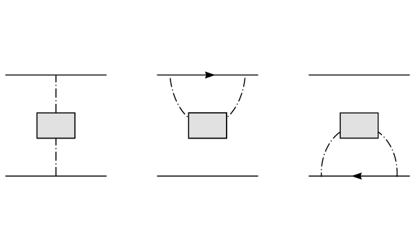
FIG. 3.: Non-perturbative contributions to the bound state kernel in QCD.

REFERENCES

• [1] M. E. Peskin, in Proceedings of the 11th SLAC Inst., SLAC Rep. n.207, 151 ed. by P. Mc. Donough (1983);
• [2] A. Barchielli, E. Montaldi and G. M. Prosperi, Nucl. Phys. B 296, 625 (1988);
• [3] Yu. A. Simonov, Nucl. Phys. B 307, 512 (1988) and B 324, 67 (1989);
• [4] W. Lucha, F. F. Schöberl and D. Gromes, Phys. Rep. 200, 127 (1990);
• [5] Yu. A. Simonov and J. A. Tjon, Ann. Phys. 228, 1 (1993);
• [6] T. Nieuwenhuis and J. A. Tjon, Phys. Lett. B 355, 283 (1995) and Phys. Rev. Lett. 77, 814 (1996);
• [7] N. Brambilla, P. Consoli and G. M. Prosperi, Phys. Rev. D 50, 5878 (1994); N. Brambilla and G. M. Prosperi, in Proceedings of “Quark Confinement and the Hadron Spectrum”, eds. N. Brambilla and G. M. Prosperi, p. 113, (World Scientific, Singapore, 1995);
• [8] N. Brambilla, E. Montaldi and G. M. Prosperi, Phys. Rev. D 54, 3506 (1996);
• [9] M. Baker, J. S. Ball, N. Brambilla, G. M. Prosperi and F. Zachariasen, Phys. Rev. D 54, 2829 (1996);
• [10] N. Brambilla and A. Vairo, Heavy quarkonia: Wilson area law, stochastic vacuum model and dual QCD, Phys. Rev. D 55, 3974 (1997); M. Baker, J. S. Ball, N. Brambilla and A. Vairo, Phys. Lett. B 389, 577 (1996);
• [11] E. Eichten and F. Feinberg, Phys. Rev. D 23, 2724 (1981);
• [12] Yu. A. Simonov, Confinement (unpublished) (1996);
• [13] C. R. Munz, J. Resag, B. C. Metsch and H. R. Petry, Nucl. Phys. A 578, 418 (1994); A. Afanesev and W. Buck, CEBAF-TH-96-12;
• [14] A. Gara, B. Durand and L. Durand, Phys. Rev. D 42, 1651 (1990); D 40, 843 (1989); J. F. Lagae, Phys. Rev. D 45, 305 (1992) and 317 (1992); N. Brambilla and G. M. Prosperi, Phys. Rev. D 48, 2360 (1993); D 46, 1096 (1992); M. G. Olsson, S. Veseli and K. Williams, Phys. Rev. D 52, 5141 (1995); J. Parramore and J. Piekarewicz, Nucl. Phys. A 585, 705 (1995);
• [15] See e.g. M. R. Frank and C. D. Roberts, Phys. Rev. C 53, 390 (1996) and references therein;
• [16] J. J. Sakurai, Modern Quantum Mechanics, ed. by The Benjamin/Cummings Publishing Company (1985);
• [17] R. P. Feynman, Phys. Rev. 80, 440 (1950); J. Schwinger, Phys. Rev. 82, 664 (1951);
• [18] K. G. Wilson, Phys. Rev. D 10, 2445 (1974);
• [19] L. Durand and E. Mendel, Phys. Lett. B 85, 241 (1979);
• [20] A. A. Migdal, Phys. Rep.102, 199 (1983);
• [21] H. G. Dosch, Phys. Lett. B 190, 177 (1987); H. G. Dosch and Yu. A. Simonov, Phys. Lett. B 205, 339 (1988);
• [22] C. Cronström, Phys. Lett. B 90, 267 (1980);
• [23] M. A. Shifman, A. I. Vainshtein and V. I. Zakharov, Nucl. Phys. B 147, 385 (1979);
• [24] H. G. Dosch, Prog. Part. Nucl. Phys. 33, 121 (1994); O. Nachtmann, Lectures given at the International University School of Nuclear and Particle Physics Schladming, Austria, (1996) HD-THEP-96-38;
• [25] M. Campostrini, A. Di Giacomo and G. Mussardo, Z. Phys. C 25, 173 (1984); A. Di Giacomo and H. Panagopoulos, Phys. Lett. B 285, 133 (1992); A. Di Giacomo, E. Meggiolaro and H. Panagopuolos, (March 1996) hep–lat/9603017;
• [26] H.G. Dosch, E. Ferreira and A. Krämer, Phys. Rev. D 50, 1992 (1994); M. Rüter and H. G. Dosch, Phys. Lett. B 380, 177 (1996);
• [27] N. Brambilla and A. Vairo, Non-perturbative dynamics of the heavy-light quark system in the non-recoil limit, HD-THEP-97-07 (1997), to appear in Phys. Lett. B.
b Refer to caption