Non-perturbative dynamics of the heavy-light quark system in the non-recoil limit

Abstract

Starting from the relativistic gauge-invariant quark-antiquark Green function we obtain the relevant interaction in the one-body limit, which can be interpreted as the kernel of a non-perturbative Dirac equation. We study this kernel in different kinematic regions, reproducing, in particular, for heavy quark the potential case and sum rules results. We discuss the relevance of the result for heavy-light mesons and the relation with the phenomenological Dirac equations used up to now in the literature.

HD-THEP-97-07

JLAB-THY-97-16

1 Introduction

In the last years a lot of efforts has gone into the study of systems involving at least one heavy quark ($Q$). On the experimental side there are a lot of data on the heavy mesons states ($Q\bar{Q}$), new data already measured [1] and a great expectation for the ones to come on the heavy-light states ($q\bar{Q}$). On the theoretical side the situation is the following. The dynamics of the systems composed by two heavy quarks is quite well understood in terms of potential interaction (static and relativistic corrections) [2, 3, 4, 5, 6, 7, 8] obtained from the semirelativistic reduction of the QCD dynamics (for lattice studies see [9]). In the heavy-light case it turns out useful to take advantage of the heavy quark symmetries [10]. Heavy-quark symmetry implies that, in the limit where $m_{Q}\gg\Lambda_{\rm QCD}$, the long-distance physics of several observables is encoded in few hadronic parameters, which in general can be defined in terms of operator matrix elements in heavy quark effective theory (HQET). For some recent reviews we refer the reader to [11]. In this framework a systematic expansion can be done in the small parameters $\Lambda_{\rm QCD}/m_{Q}$ and $\alpha_{\rm s}(m_{Q})$. In the limit $m_{Q}\to\infty$ all the physics can be expressed in terms of a small number of form factors depending on the light quark and gluon dynamics only. Then, in HQET the heavy-light meson mass is given by

$$m_{M}=m_{Q}+\bar{\Lambda}+O\left({1\over m_{Q}}\right)\,\,{\rm corrections}$$ (1)

The parameter $\bar{\Lambda}$ represents contributions coming from all terms independent of the heavy-quark mass $m_{Q}$; it is one of the non-perturbative parameters of the HQET, which have a similar status as the vacuum condensates in sum rules and QCD phenomenology. $\bar{\Lambda}$ can be fixed on the data, its actual calculation however needs a dynamical input. Of course the dynamics of the light quark is inerehently non-perturbative. Some approaches resort to dynamical calculation via phenomenological potential models [12, 13], sum rules [14] or relativistic phenomenological equations [15]. To have a well founded calculation of $\bar{\Lambda}$ is of great importance since its value affects the determination of many phenomenological quantities (cf e. g. [16]).

In this letter we address the question of calculating the non-recoil corrections to the heavy-light mesons ($\bar{\Lambda}$) via a Dirac equation justified by the QCD dynamics. Our starting point is the quark-antiquark gauge-invariant Green function taken in the infinite mass limit of one particle. The only dynamical assumption is on the behaviour of the Wilson loop. The gauge invariance of the formalism guarantees that the relevant physical information are preserved at any step of our derivation. In this way we obtain a QCD justified fully relativistic interaction kernel for the quark in the infinite mass limit of the antiquark. This kernel reduces in some region of the physical parameters to the heavy quark mass potential, and leads in some other region to the heavy quark sum rules results, providing in this way an unified description. In the light of our result we scrutinize the phenomenological Dirac equations used in the literature and give an answer to the old-standing problem of the Lorentz structure of the Dirac kernel for a confining interaction [15, 17, 18, 19].

There are many possible applications of the obtained result, like the study of relativistic properties of the spectrum (as much relevant as the quark is light) and the calculation of heavy-light meson matrix elements and form factors (e. g. the Isgur–Wise function). Finally, this work can also be intended as a step forward both in the direction of a theory derived two-body relativistic interaction, both in the direction of a generalization of the sum rules approach with the inclusion of a finite gluon correlation length.

2 The one-body interaction

The quark-antiquark Green function is given in quenched approximation by

$$G_{\rm inv}(x,u,y,v)=\left\langle{\rm Tr}\,i\,S^{(1)}(x,y;A)U(y,v)\,i\,S^{(2)}(v,u;A)U(u,x)\right\rangle,$$ (2)

where the points $x,y,u,v$ are defined as in Fig. 1, $\langle~{}~{}\rangle$ means the normalized average over the gauge field $A_{\mu}$, $S^{(i)}$ is the fermion propagator in the external field $A_{\mu}$ associated with the particle $i$ and the strings $U(y,x)\equiv{\rm P}\,\exp\left\{\displaystyle ig\int_{0}^{1}ds\,(y-x)^{\mu}A_{\mu}(x+s(y-x))\right\}$ are needed in order to have gauge invariant initial and final bound states. A very convenient way to represent it is the so-called Feynman–Schwinger representation (see [20, 21] and refs. therein), where the fermion propagators are expressed in terms of quantomechanical path integrals over the quark trajectories ($z_{1}(t_{1})$ and $z_{2}(t_{2})$)

$$G_{\rm inv}(x,u,y,v)={1\over 4}\Bigg{\langle}{\rm Tr}\,{\rm P}\,(i\,{D\!\!\!\!/}_{y}^{\,(1)}+m_{1})\,\int_{0}^{\infty}dT_{1}\int_{x}^{y}{\cal D}z_{1}e^{\displaystyle-i\,\int_{0}^{T_{1}}dt_{1}{m^{2}+\dot{z}_{1}^{2}\over 2}}$$ (3)

$$\qquad\quad\times\int_{0}^{\infty}dT_{2}\int_{v}^{u}{\cal D}z_{2}e^{\displaystyle-i\,\int_{0}^{T_{2}}dt_{2}{m^{2}+\dot{z}_{2}^{2}\over 2}}e^{\displaystyle ig\oint_{\Gamma}dz^{\mu}A_{\mu}(z)}$$

$$\qquad\quad\times e^{\displaystyle i\,\int_{0}^{T_{1}}dt_{1}{g\over 4}\sigma_{\mu\nu}^{(1)}F^{\mu\nu}(z_{1})}e^{\displaystyle i\,\int_{0}^{T_{2}}dt_{2}{g\over 4}\sigma_{\mu\nu}^{(2)}F^{\mu\nu}(z_{2})}(-i\,\buildrel\leftarrow\over{D\!\!\!\!/}_{v}^{\,(2)}+m_{2})\Bigg{\rangle}.$$

From Eq. (3) it emerges quite manifestly that the entire dynamics of the system depends on the Wilson loop:

$$W(\Gamma;A)\equiv{\rm Tr\,}{\rm P\,}\exp\left\{ig\oint_{\Gamma}dz^{\mu}A_{\mu}(z)\right\},$$ (4)

being $\Gamma$ the closed curve defined by the quark trajectories and the endpoint strings $U(y,v)$ and $U(u,x)$.

Let us assume that the antiquark moving on the second fermion line becomes infinitely heavy. The only trajectory surviving in the path integral of Eq. (3) associated with the second particle is the static straight line propagating from $v$ to $u$. The corresponding Wilson loop of the system is represented in Fig. 1. As already noted in [22] in this case it turns out to be very convenient to choose the following gauge condition (sometimes called modified coordinate gauge):

$$A_{\mu}(x_{0},{\bf 0})=0,\qquad\qquad x^{j}A_{j}(x_{0},{\bf x})=0.$$

Thanks to this gauge choice it is possible to express the gauge field in terms of the field strength tensor,

$$A_{0}(x) = \int_{0}^{1}d\alpha\,x^{k}F_{k0}(x_{0},\alpha{\bf x}),$$

$$A_{j}(x) = \int_{0}^{1}d\alpha\,\alpha\,x^{k}F_{kj}(x_{0},\alpha{\bf x}).$$

Moreover the only non-vanishing contribution to the Wilson loop is given by the quark paths connecting $x$ with $y$, and we have

$$W(\Gamma;A)={\rm Tr\,}{\rm P\,}\exp\left\{ig\int_{x}^{y}dz^{\mu}A_{\mu}(z)\right\}.$$ (5)

We stress that the choice of the gauge is in this approach really arbitrary and motivated only by convenience. Being the formalism completely gauge invariant, by handling properly we would obtain exactly the same results within any gauge.

b

Figure 1: The Wilson loop in the static limit of the heavy quark.

As showed in [20, 21] in order to evaluate Eq. (3) we need to know the Wilson loop average over the gauge fields. We evaluate it via the cumulant expansion described in [4]. Keeping only bilocal cumulants we obtain:

$$\langle W(\Gamma,A)\rangle = \exp\left\{-{g^{2}\over 2}\int_{x}^{y}dx^{\prime\mu}\int_{x}^{y}dy^{\prime\nu}D_{\mu\nu}(x^{\prime},y^{\prime})\right\},$$

$$D_{\mu\nu}(x,y) \equiv x^{k}y^{l}\int_{0}^{1}d\alpha\,\alpha^{n(\mu)}\int_{0}^{1}d\beta\,\beta^{n(\nu)}\langle F_{k\mu}(x^{0},\alpha{\bf x})F_{l\nu}(y^{0},\beta{\bf y})\rangle,$$ (6)

where $n(0)=0$ and $n(i)=1$. Assumption (6) corresponds to the so-called stochastic vacuum model and has been very successful in the last years either in applications to potential models as well as in the study of soft high energy scattering problems (for some recent reviews see [23]). Inserting expression (6) in Eq. (3) and expanding the exponential we obtain the following expression for the propagator $S_{D}$ of the quark ($S_{D}$ is $G_{\rm inv}$ “projected” on the first fermion line; the second quark is irrelevant in the infinite mass limit, playing the role of an external source):

$$S_{D}=S_{0}+S_{0}\,K\,S_{0}+S_{0}\,K\,S_{0}\,K\,S_{0}+\cdots.$$ (7)

$S_{0}$ is the free fermion propagator. Taking into account only the first planar graph (since we are interested only in contributions proportional to the gluon condensate), we have $K(y^{\prime},x^{\prime})=\gamma^{\nu}S_{0}(y^{\prime},x^{\prime})\gamma^{\mu}D_{\mu\nu}(x^{\prime},y^{\prime})$. A graphical representation of $K$ is given in Fig. 2. Eq. (7) can be written in closed form as $S_{D}=S_{0}+S_{0}KS_{D}$ (or in terms of wave-function, $({p\!\!\!/}-m-iK)\psi=0$; $m\equiv m_{1}$). Therefore, $K$ can be interpreted as the interaction kernel of the Dirac equation associated with the motion of a quark in the field generated by an infinitely heavy antiquark.

b

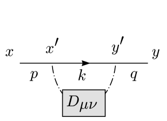
Figure 2: The interaction kernel $K$.

Assuming that the correlator $\langle F_{\mu\lambda}(x)F_{\nu\rho}(y)\rangle$ depends only on the difference between the coordinates, we define:

$$\langle F_{k\mu}(x^{0},\alpha{\bf x})F_{l\nu}(y^{0},\beta{\bf y})\rangle\equiv f_{k\mu l\nu}(x^{0}-y^{0},\alpha{\bf x}-\beta{\bf y}).$$

With this assumption $K$ can be written in momentum space as (see Fig. 2 for the definition of the momenta):

$$K(q,p) = -g^{2}(2\pi)\delta(p^{0}-q^{0})$$ (8)

$$\times \int_{-\infty}^{+\infty}d\tau\int_{0}^{1}d\alpha\,\alpha^{n(\mu)}\int_{0}^{1}d\beta\,\beta^{n(\nu)}{\partial\over\partial p^{k}}{\partial\over\partial q^{l}}\int d^{3}r\,e^{i({\bf p}-{\bf q})\cdot{\bf r}}$$

$$\times \gamma^{\nu}\left\{\theta(-\tau)\Lambda_{+}({\bf t})\gamma^{0}e^{-i(p^{0}-E_{t})\tau}-\theta(\tau)\Lambda_{-}({\bf t})\gamma^{0}e^{-i(p^{0}+E_{t})\tau}\right\}\gamma^{\mu}$$

$$\times f_{k\mu l\nu}(\tau,(\alpha-\beta){\bf r}),$$

where ${\bf t}\equiv(\beta{\bf p}-\alpha{\bf q})/(\beta-\alpha)$, $E_{t}=\sqrt{t^{2}+m^{2}}$ and $\Lambda_{\pm}({\bf t})={\displaystyle{E_{t}\pm(m-{\bf t}\cdot\gamma)\gamma^{0}\over 2E_{t}}}$.

Equation (8) is our basic expression. It contains the perturbative interaction up to order $g^{2}$ and the non-perturbative one carried by a single insertion of a second order cumulant. From now on we want to focus our attention only on the purely non-perturbative interaction. The Lorentz structure of the non-perturbative relevant part of $f_{\mu\lambda\nu\rho}$ is

$$f^{\rm n.p.}_{\mu\lambda\nu\rho}(x)={1\hskip-2.2pt{\rm l}}_{\rm c}\,{\langle F^{2}(0)\rangle\over 24N_{c}}(g_{\mu\nu}g_{\lambda\rho}-g_{\mu\rho}g_{\lambda\nu})D(x^{2}),$$ (9)

where $\langle F^{2}(0)\rangle$ is the gluon condensate, ${1\hskip-2.2pt{\rm l}}_{\rm c}$ the identity matrix of SU(3) and $D$ is a non-perturbative form factor normalized to unit at the origin. Lattice simulations have showed that $D$ falls off exponentially (in Euclidean space-time) at long distances with a correlation length $a^{-1}\sim(1~{}{\rm GeV})^{-1}$ [24]. This behaviour of $D$ is sufficient to give confinement, at least in some kinematic regions [4]. Moreover we notice that, if $f^{\rm n.p.}_{\mu\lambda\nu\rho}\sim{\displaystyle e^{-ia\tau}}$, then we have

$$K\sim{\partial\over\partial p^{k}}{\partial\over\partial q^{l}}\int d^{3}r\,e^{i({\bf p}-{\bf q})\cdot{\bf r}}\gamma^{\nu}S_{0}(p_{0}+a,{\bf t})\gamma^{\mu}f^{\rm n.p.}_{k\mu l\nu}(0,(\alpha-\beta){\bf r}).$$

The main effect of the finite correlation length $a^{-1}$ seems to consist, therefore, in a shifting of the pole in the inserted free fermion propagator.

In the following we will study expression (8) for different choices of the parameters which are the correlation length $a$, the mass $m$, the binding energy $(p_{0}-m)$ and the momentum transfer $({\bf p}-{\bf q})$.

A. Heavy quark potential case ($m>a>p_{0}-m$)

If we assume $a$ to be bigger than the binding energy $(p_{0}-m)$ and smaller than the mass $m$ of the quark, since $a\sim 1$ GeV, the quark turns out to be sufficiently heavy to be considered non-relativistic. In order to obtain the $1/m^{2}$ potential we can neglect the “negative energy states” contributions to (8) by writing

$$K(q,p) \simeq -g^{2}(2\pi)\delta(p^{0}-q^{0})$$ (10)

$$\times \int_{0}^{+\infty}d\tau\int_{0}^{1}d\alpha\,\alpha^{n(\mu)}\int_{0}^{1}d\beta\,\beta^{n(\nu)}{\partial\over\partial p^{k}}{\partial\over\partial q^{l}}\int d^{3}re^{i({\bf p}-{\bf q})\cdot{\bf r}}$$

$$\times \gamma^{\nu}\Lambda_{+}({\bf t})\gamma^{0}\gamma^{\mu}f^{\rm n.p.}_{k\mu l\nu}(\tau,(\alpha-\beta){\bf r}).$$

Now, inserting Eq. (9) and by means of usual reduction techniques [25], we obtain up to order $1/m^{2}$ the static and spin dependent potential

$$V(r) = g^{2}{\langle F^{2}(0)\rangle\over 24N_{c}}\int_{-\infty}^{+\infty}d\tau\int_{0}^{r}d\lambda\,(r-\lambda)\,D(\tau^{2}-\lambda^{2})$$ (11)

$$+ {{\bf\sigma}\cdot{\bf L}\over 4m^{2}}{1\over r}g^{2}{\langle F^{2}(0)\rangle\over 24N_{c}}\int_{-\infty}^{+\infty}d\tau\int_{0}^{r}d\lambda\left(2{\lambda\over r}-1\right)D(\tau^{2}-\lambda^{2}),$$

where we have make use of the change of variable $\lambda=(\alpha-\beta)|{\bf r}|$. This result agrees with the one body limit of the potential given in [4, 6]. In particular for $r\to\infty$ identifying the string tension $\sigma=\displaystyle g^{2}{\langle F^{2}(0)\rangle\over 24N_{c}}\int_{-\infty}^{+\infty}d\tau\int_{0}^{\infty}d\lambda\,D(\tau^{2}-\lambda^{2})$ we obtain the well-known Eichten and Feinberg result [2],

$$V(r)=\sigma r-C-{{\bf\sigma}\cdot{\bf L}\over 4m^{2}}\,\,{\sigma\over r},$$ (12)

where $C$ is the constant term $\displaystyle g^{2}{\langle F^{2}(0)\rangle\over 24N_{c}}\int_{-\infty}^{+\infty}d\tau\int_{0}^{\infty}d\lambda\,\lambda\,D(\tau^{2}-\lambda^{2})$. We observe that the Lorentz structure which gives origin to the negative sign in front of the spin-orbit potential in (12) is in our case not simply a scalar ($K\simeq\sigma\,r$). We will discuss this point in more detail in the conclusions.

B. Sum rules case ($a<p_{0}-m$, $a<m$)

Let us consider now the case in which the binding energy of the quark is bigger than the correlation length, which can be considered zero respect to all the scales of the problem. In the literature is usually referred to this case as the non potential case [4]. Since $f^{\rm n.p.}_{\mu\lambda\nu\rho}(x){\displaystyle{\mathop{\longrightarrow}\limits_{a\to 0}}}f^{\rm n.p.}_{\mu\lambda\nu\rho}(0)$ $={1\hskip-2.2pt{\rm l}}_{\rm c}\langle F^{2}(0)\rangle/24N_{c}(g_{\mu\nu}g_{\lambda\rho}-g_{\mu\rho}g_{\lambda\nu})$, we have

$$K(q,p) \simeq -g^{2}(2\pi)\delta(p^{0}-q^{0}){1\hskip-2.2pt{\rm l}}_{\rm c}{\langle F^{2}(0)\rangle\over 24N_{c}}(g_{\mu\nu}g_{kl}-g_{\mu l}g_{\nu k})$$ (13)

$$\times \int_{0}^{1}d\alpha\,\alpha^{n(\mu)}\int_{0}^{1}d\beta\,\beta^{n(\nu)}{\partial\over\partial p^{k}}{\partial\over\partial q^{l}}\left(\gamma^{\nu}S_{0}(p)\gamma^{\mu}(2\pi)^{3}\delta^{3}({\bf p}-{\bf q})\right).$$

In particular from Eq. (13) we obtain the well-known leading contribution to the heavy quark condensate [26]:

$$\langle\bar{Q}Q\rangle=-\int{d^{4}p\over(2\pi)^{4}}\int{d^{4}q\over(2\pi)^{4}}{\rm Tr}\left\{S_{0}(q)K(q,p)S_{0}(p)\right\}=-{1\over 12}{\langle\alpha F^{2}(0)\rangle\over\pi m}.$$

C. Light quark case ($a>m$)

Since we have reproduced the known results concerning heavy quarks, Eq. (8) should maintain some physical meaning also by considering heavy-light mesons with a strange quark (like D_s and B_s). In this case the light quark mass is smaller than $a$: $m_{\rm s}\sim$ 200 MeV $<1$ GeV. Actually the case $a>m$ has to be considered as the only realistic one concerning heavy-light mesons. Under this condition either the exponent $(p_{0}-E_{t})$ as well as $(p_{0}+E_{t})$ can be neglected with respect to $a$. Therefore we have:

$$K(q,p) \simeq -g^{2}(2\pi)\delta(p^{0}-q^{0})$$ (14)

$$\times \int_{0}^{+\infty}d\tau\int_{0}^{1}d\alpha\,\alpha^{n(\mu)}\int_{0}^{1}d\beta\,\beta^{n(\nu)}{\partial\over\partial p^{k}}{\partial\over\partial q^{l}}\int d^{3}re^{i({\bf p}-{\bf q})\cdot{\bf r}}$$

$$\times \gamma^{\nu}\left({m-{\bf t}\cdot\gamma\over E_{t}}\right)\gamma^{\mu}f^{\rm n.p.}_{k\mu l\nu}(\tau,(\alpha-\beta){\bf r}).$$

We observe, as an appealing feature of this expression, that in the zero mass limit it gives a chirally symmetric interaction (while a purely scalar interaction breaks chiral symmetry at any mass scale). On the other hand, by considering only its static contribution (i. e. neglecting all momentum dependent terms), we obtain (using the same definition of the string tension given previously):

$$K(q,p)\big{|}_{\rm static}=g^{2}(2\pi)\delta(p^{0}-q^{0})\,\int d^{3}re^{i({\bf p}-{\bf q})\cdot{\bf r}}{5\over 3}\,\sigma\,r.$$

The factor $5/3$ in front of $\sigma$ which arises naturally in this approach under the considered physical conditions, seems to supply an explanation for the fact, observed by many authors [15, 17, 18], that in order to reproduce the D_s and B_s spectra from a Dirac equation with scalar confinement a string tension almost twice respect to the usual value is needed.

3 Conclusions

In the literature, also recently, a Dirac equation with scalar confining kernel (i. e. $K\simeq\sigma\,r$) has been used in order to calculate non-recoil contributions to the heavy-light meson spectrum [15, 17, 18]. The main argument in favor of this type of kernel is the nature of the spin-orbit potential for heavy quarks. This turns out to have a long-range vanishing magnetic contribution (according to the Buchmüller picture of confinement) and is completely described by the Thomas precession term. This situation is compatible with a scalar confining kernel. However, assuming more sophisticated confinement models with a bigger sensitivity to the intermediate distance region, the spin-orbit interaction has no more such a simple behaviour. In particular there show up non zero corrections to the magnetic spin orbit potential. Moreover, the velocity dependent sector of the potential seems not to be compatible with a scalar kernel (we refer the reader to [6] for an exhaustive discussion). Therefore also from the point of view of the potential theory there are strong indications that the Lorentz structure of the confining kernel should be more complicate that a simple scalar one. This emerges also in our approach. The kernel (8) follows simply from the assumption on the gauge fields dynamics given by Eq. (6). In principle all the graphs constructed by inserting non-perturbative gluon propagators on the quark fermion line should be taken into account. Since we are interested only in terms proportional to $\sigma$ (or $\langle F^{2}(0)\rangle$), we keep only the first one. When performing the potential reduction of this kernel in the heavy quark case (A) we obtain exactly the expected static and spin-dependent potentials. Therefore our conclusion is that there exists at least one non scalar kernel which reproduces for heavy quark not only the Eichten and Feinberg potentials in the long distances limit, but also the entire stochastic vacuum model spin dependent potential. Moreover when considering $a$, the inverse of the correlation length, small with respect to all the energy scales (case B), the kernel (8) gives back the leading heavy quark sum rules results. It is possible to try to extend the range of applicability of Eq. (8) to more realistic cases, like D_s and B_s mesons where the light quark mass is smaller than the characteristic correlation length of the two point cumulant (case C). The relevant part of the kernel is also in this case not a simply scalar one. In the static approximation this kernel seems, indeed, to be compatible with the existing phenomenology. We notice, however, that the situation is quite different from QED where in the Coulomb gauge a static interaction emerges without any approximation since the transverse part of the propagator of the exchanged photon (the relevant contribution to the binding) vanishes when the second fermion line is taken infinitely heavy. In our approach a purely static contribution never emerges, being relevant to the binding not an exchange graph between the quarks, but the interaction with the background vacuum fields. Therefore any static approximation in a real heavy-light system, for which the light quark is expected to be far from a static one, appears doubtful.

Acknowledgments The authors gratefully acknowledge the Jefferson Lab Theory Group as well as the Hampton University for their warm hospitality during the first stage of this work, the Alexander von Humboldt Foundation for support and D. Gromes for useful discussions. This work was supported in part by NATO grant under contract N. CRG960574.

References

- [1] Particle Data Group, R. M. Barnett et. al., Phys. Rev. D 54 (1996) 1;
- [2] K. G. Wilson, Phys. Rev. D 10 (1974) 2445; E. Eichten and F. Feinberg, Phys. Rev. D 23 (1981) 2724; see also e.g. E. Eichten, in ”Lattice ’90”, eds. V. A. Heller et al., Nucl. Phys. B 20 (Proc. Suppl.) (1991) 475;
- [3] A. Barchielli, E. Montaldi and G. M. Prosperi, Nucl. Phys. B 296 (1988) 625; N. Brambilla, P. Consoli and G. M. Prosperi, Phys. Rev. D 50 (1994) 5878;
- [4] H. G. Dosch, Phys. Lett. B 190 (1987) 177; H. G. Dosch and Yu. A. Simonov, Phys. Lett. B 205 (1988) 339; Yu. A. Simonov, Nucl. Phys. B 307 (1988) 512; B 324 (1989) 67;
- [5] M. Baker, J. S. Ball and F. Zachariasen, Phys. Rev. D 51 (1995) 1968; M. Baker, J. S. Ball, N. Brambilla, G. M. Prosperi and F. Zachariasen, Phys. Rev. D 54 (1996) 2829;
- [6] N. Brambilla and A. Vairo, Phys. Rev. D 55 (1997) 3974; M. Baker, J. Ball, N. Brambilla and A. Vairo, Phys. Lett. B 389 (1996) 577;
- [7] S. Titard and F. J. Yndurain, Phys. Rev. D 49 (1994) 6007; D 51 (1995) 6348; A. Pineda and J. Soto, Phys. Rev. D 54 (1996) 4609;
- [8] Yu-Qi Chen and R. Oakes, Phys. Rev. D 53 (1996) 5051;
- [9] See e. g. C. Davies in “Quark Confinement and the Hadron Spectrum II”, eds. N. Brambilla and G. M. Prosperi, (World Scientific, Singapore, 1997) and references therein;
- [10] N. Isgur and M. Wise, Phys. Lett. B 232 (1989) 113;
- [11] M. Neubert, Lectures given at the International School of Subnuclear Physics: 34th Course: Effective Theories and Fundamental Interactions, Erice, Italy, (1996) CERN-TH-96-281; Phys. Rep. 245 (1994) 259; T. Mannel in “Schladming 1996, Perturbative and nonperturbative aspects of quantum field theory”, (Springer, Berlin, 1996); B. Grinstein, Lectures given at 6th Mexican School of Particles and Fields, Villahermosa, Mexico, (1994);
- [12] E. J. Eichten, C. Hill and C. Quigg, Phys. Rev. Lett. D 71 (1993) 4116;
- [13] W. Kwong and J. Rosner, Phys. Rev. D 44 (1991) 212 and refs. therein;
- [14] M. Neubert, Phys. Rev. D 46 (1992) 1076; E. Bagan, P. Ball, V. M. Braun and H. G. Dosch, Phys. Lett. B 278 (1992) 457;
- [15] M. R. Ahmady, R. Mendel and J. D. Talman, Phys. Rev. D 52 (1995) 254;
- [16] I. I. Bigi and N. G. Uraltsev, Z. Phys. C 62 (1994) 623;
- [17] V. D. Mur, V. S. Popov, Yu. A. Simonov and V. P. Yurov, J. Expt. Theor. Phys. 78 (1994) 1;
- [18] M. G. Olsson, S. Veseli and K. Williams, Phys. Rev. D 51 (1995) 5079;
- [19] G. Hardekopf and J. Sucher, Phys. Rev. A 30 (1984) 703; A 31 (1985) 2020;
- [20] Yu. A. Simonov and J. A. Tjon, Ann. Phys. 228 (1993) 1;
- [21] N. Brambilla and A. Vairo, From the Feynman–Schwinger representation to the non-perturbative relativistic bound state interaction, HD-THEP-97-08 (1997)/ JLAB-THY-97-17, to appear in Phys. Rev. D 56;
- [22] I. I. Balitsky, Nucl. Phys. B 254 (1985) 166;
- [23] H. G. Dosch, Prog. Part. Nucl. Phys. 33 (1994) 121; O. Nachtmann, in “Schladming 1996, Perturbative and nonperturbative aspects of quantum field theory”, (Springer, Berlin, 1996);
- [24] M. Campostrini, A. Di Giacomo and G. Mussardo, Z. Phys. C 25 (1984) 173; A. Di Giacomo and H. Panagopoulos Phys. Lett. B 285 (1992) 133; A. Di Giacomo, E. Meggiolaro and H. Panagopoulos, (March 1996) hep-lat/9603017;
- [25] W. Lucha, F. F. Schöberl and D. Gromes, Phys. Rep. 200 (1990) 127;
- [26] M. A. Shifman, A. I. Vainshtein and V. I. Zakharov, Nucl. Phys. B 147 (1979) 385.