Dimensionally Regularized Box and Phase-Space Integrals Involving Gluons and Massive Quarks

Abstract

The basic box and phase-space integrals needed to compute at second order the three-jet decay rate of the $Z$-boson into massive quarks are presented in this paper. Dimensional regularization is used to regularize the infrared divergences that appear in intermediate steps. Finally, the cancellation of these divergences among the virtual and the real contributions is showed explicitly.

12.15.Ff, 12.38.Bx, 12.38.Qk, 13.38.Dg, 14.65.Fy

I Introduction

In higher order QCD calculations at LEP the effects of quark masses are always screened by the ratio $m_{q}^{2}/s$, where $m_{q}$ is the mass of the quark and $s$ is the center of mass energy. At LEP, even for the heaviest produced quark, the bottom quark, we have $(m_{b}/m_{Z})^{2}\sim 0.003$ and, therefore, for inclusive observables, such as total hadronic cross section, or the decay width of $Z\rightarrow\bar{b}b$, the mass effects are almost negligible. The situation is different for more exclusive observables. It has been stressed [1] that quark mass effects could be enhanced in jet production cross sections. In this case observables depend also on a new variable, $y_{c}$, the jet-resolution parameter that defines the multiplicity of the jets. In fact, these effects have already been seen [2]. However, it has also been shown in [1] that second-order QCD predictions are necessary in order to perform a meaningful comparison of the theory with experimental results and to possibly extract the value of the quark mass from such measurements.

In previous papers [3] we have presented the results of the calculation of some three-jet fractions at LEP including next-to-leading (NLO) corrections and keeping the full dependence on the $b$-quark mass. In this paper we focus on several technical details that appear in the calculation. Our results for some IR divergent integrals with massive quarks are new and could be used in many other calculations of this type.

The main difficulty of the NLO calculation is the appearance, in addition to ultraviolet (UV) divergences, of infrared (IR) singularities because gluons are massless. The Bloch-Nordsieck (BN) and Kinoshita-Lee-Nauenberg (KLN) theorems [4] assure that jet cross-sections are infrared finite and free from collinear divergences. The IR singularities of the NLO one-loop Feynman diagrams cancel against the IR divergences that appear when the differential cross-section for four-parton production is integrated over the region of phase-space where either one gluon is soft or two gluons are collinear. Nevertheless, infrared and collinear divergences appear in intermediate steps and should be treated properly. We used dimensional regularization to regularize both UV and IR divergences [5] because it preserves the QCD Ward identities.

For massive quarks, the gluon-quark collinear singularities, that appear in the massless case, are softened into logarithms of the quark mass. The number of IR singularities is, therefore, smaller. However, quark masses complicate extremely the loop and phase-space integrals. In particular, diagrams containing gluon-gluon collinear divergences are much harder to calculate than in the massless case. Furthermore, infrared singularities appear always at the border of the integration region. For virtual contributions, at the border of the one unit side box defined by the Feynman parameters. For contributions coming from the emission of real gluons, at the border of the phase-space. Thus, any simplification is impossible, the full calculation has to be performed in arbitrary $D=4-2\epsilon$ dimensions and expansions for $\epsilon\rightarrow 0$ are allowed only at the end.

Several methods of analytical cancellation of infrared singularities have been developed in the past. The most popular are the phase-space slicing method [6] and the subtraction method [7, 8, 9]. We work in the context of the so-called phase-space slicing method. In this case the analytical integration over a thin slice at the border of the phase-space is performed in $D$-dimensions and the result is added to the virtual corrections. The integration over the rest of the phase-space, which is finite, is done numerically for $D=4$.

The structure of this paper is as follows. In section II we consider the most complicated, IR divergent one-loop box integrals that appear in the calculation of the three-jet decay rate of the $Z$-boson into massive quarks at NLO. We start this section by presenting the calculation of some simpler three-point scalar integrals, which control the IR structure of the box diagrams. One of the box integrals involves the three-gluon vertex and was only known in the case of massless quarks [10]. We have calculated it also for the massive case by using dimensional regularization. This is one of the main contributions of this paper.

Section III is devoted to the calculation of the basic phase-space integrals of the $Z$-decay into four partons wich lead to IR (collinear) divergent contributions to the three-jet fractions. We used the phase-space slicing method. When one of the gluons is soft, the calculation is performed by imposing a theoretical cut on the energy of the gluon, $E_{3}<w$. The $w$-cut should be small enough to allow for expansions for small $w$ in the analytical calculations and should not interfere with the experimental cuts. On the other hand, it should be large enough to avoid instabilities in the numerical integrations. For the transition amplitudes containing gluon-gluon collinear divergences we perform the cut on $y_{34}=2(p_{3}\cdot p_{4})/s$, the scalar product of the momenta of the two gluons normalized to the center of mass energy. These contributions have to cancel exactly the appropriate infrared poles of the virtual contributions. We show explicitly how these basic integrals share the same infrared behavior as the one-loop scalar functions considered in section II. Finally, in appendices A and B, we collect some properties of the hypergeometric functions and the formulae that define the three- and the four-body phase-space in arbitrary space-time $D$-dimensions.

Throughout all this paper we work with the following set of dimensionless Lorentz-invariant variables

$$\qquad y_{ij}=2(p_{i}\cdot p_{j})/s,\qquad r_{b}=m_{b}^{2}/s,$$ (1)

where the $y_{ij}$ are the scalar product of all the possible pairs of final state momenta normalized to $s=q^{2}$, the total center of mass energy, $p_{1}^{2}=p_{2}^{2}=m_{b}^{2}$ is the mass of the quark/antiquark (in particular the $b$-quark mass) and particles labeled as 3 and 4 represent the gluons, $p_{3}^{2}=p_{4}^{2}=0$. Energy-momentum conservation imposes the following restrictions

$$y_{12} = 1-2r_{b}-y_{13}-y_{23},$$ (2)

$$y_{12} = 1-2r_{b}-y_{13}-y_{14}-y_{23}-y_{24}-y_{34}.$$ (3)

in the case of the decays $Z\rightarrow b\bar{b}g$ and $Z\rightarrow b\bar{b}gg$ respectively.

II One-loop integrals contributing to three-parton final states

We consider here the IR divergent virtual corrections to the three-parton decay $q\rightarrow p_{1}+p_{2}+p_{3}$ with all external particles on-shell, see fig 2.

Using the Passarino-Veltman [11] procedure we can reduce any set of vectorial or tensorial one-loop integrals to n-point scalar functions. Therefore only scalar integrals [12] have to be computed. At the NLO the relevant one-loop Feynman diagrams contribute only through their interference with the lowest order Born amplitudes. Therefore, we will be interested only in the real part of such n-point scalar one-loop integrals. Although we will not specify it, the following results refer, in almost all cases, just to the real part of these functions.

A Three-point functions

First we present results for the two three-point functions which actually define the non-trivial IR structure of the whole virtual radiative corrections for the process. As we will show below, the IR poles of the four-point functions contributing to our process are also controlled by these simpler three-point functions. Thus, we have to consider the following scalar one loop integrals, see fig 1,

$$\frac{i}{16\pi^{2}}C03(y_{13})=\mu^{4-D}$$ (4)

$$\times\int\frac{d^{D}k}{(2\pi)^{D}}\frac{1}{k^{2}(k-p_{3})^{2}[(k+p_{1})^{2}-m_{b}^{2}]}~{},$$ (5)

and

$$\frac{i}{16\pi^{2}}C05(y_{12})=\mu^{4-D}$$ (6)

$$\times\int\frac{d^{D}k}{(2\pi)^{D}}\frac{1}{k^{2}[(k+p_{1})^{2}-m_{b}^{2}][(k-p_{2})^{2}-m_{b}^{2}]}~{}.$$ (7)

In general, this kind of functions depend on all the masses in the propagators, on the square of the difference of the two external momenta and on the square of the external momenta itself. Since we have fixed the mass and we have imposed the on-shell condition the only remaining relevant arguments of these functions are the two-momenta invariants $y_{13}$ and $y_{12}$, respectively.

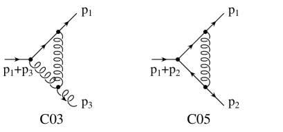
FIG. 1.: Infrared divergent triangle Feynman diagrams.

For the $C03$ function, which has a double IR pole, the most convenient Feynman parametrization is the one with both Feynman parameters running from $0$ to $1$ because then the two integrations decouple. After performing the integration over the loop momenta we have

$$C03(y_{13})=-s^{-1-\epsilon}\mu^{2\epsilon}(4\pi)^{\epsilon}\Gamma(1+\epsilon)\int_{0}^{1}x^{-1-2\epsilon}dx$$ (8)

$$\times\int_{0}^{1}\left[(1-y)(r_{b}-y(r_{b}+y_{13}))-i\eta\right]^{-1-\epsilon}dy~{}.$$ (9)

We see from here that, as we mentioned, the infrared problem is at the border of the Feynman parameter space, in this particular case at $x=0$ and $y=1$. The full calculation has to be performed for arbitrary $\epsilon$ values.

We will omit the $i\eta$ term in the following calculations, however, when needed, we will use the prescription $r_{b}\rightarrow r_{b}-i\eta$, $y_{13}\rightarrow y_{13}+i\eta$ to resolve the ambiguities.

After integration over the x-parameter we are left with

$$C03(y_{13})=s^{-1-\epsilon}\mu^{2\epsilon}(4\pi)^{\epsilon}\frac{\Gamma(1+\epsilon)}{2\epsilon}(r_{b}+y_{13})^{-1-\epsilon}$$ (10)

$$\times\int_{0}^{1}(1-y)^{-1-\epsilon}(y_{0}-y)^{-1-\epsilon}dy~{},$$ (11)

where $y_{0}=r_{b}/(r_{b}+y_{13})$. The last integral gives rise to a hypergeometric function, eq. (A1),

$$C03(y_{13})=s^{-1-\epsilon}\mu^{2\epsilon}\frac{(4\pi)^{\epsilon}}{\Gamma(1-\epsilon)}\frac{\Gamma(1+\epsilon)\Gamma(-\epsilon)}{2\epsilon}$$ (12)

$$\times(r_{b}+y_{13})^{-1-\epsilon}y_{0}^{-1-\epsilon}{}_{2}F_{1}[1+\epsilon,1;1-\epsilon;\frac{1}{y_{0}}]~{},$$ (13)

that, after some mathematical manipulations (see appendix A) can be written in terms of a dilogarithm function,

$${}_{2}F_{1}[1+\epsilon,1;1-\epsilon;\frac{1}{y_{0}}]=$$ (14)

$$\left(1-\frac{1}{y_{0}}\right)^{-1-2\epsilon}\left[1+2\epsilon^{2}Li_{2}\left(\frac{1}{y_{0}}\right)+O(\epsilon^{3})\right]~{}.$$ (15)

Above we used eq. (A3) and eq. (A4). In the region of physical interest $y_{0}$ is smaller than one, therefore to extract the real parts we transform $Li_{2}(1/y_{0})$ in terms of $Li_{2}(y_{0})$ by using the known properties of the dilogarithm function [13]. The ambiguities are solved by using the correct $i\eta$ prescription.

The final result we obtain for the real part is,

$$C03(y_{13}) = s^{-1-\epsilon}\mu^{2\epsilon}\frac{(4\pi)^{\epsilon}}{\Gamma(1-\epsilon)}\frac{1}{y_{13}}$$ (16)

$$\times \left[\frac{1}{2\epsilon^{2}}+\frac{1}{2\epsilon}\log\frac{r_{b}}{y_{13}^{2}}+\frac{1}{4}\log^{2}\frac{r_{b}}{y_{13}^{2}}\right.$$ (17)

$$- \left.\frac{1}{2}\log^{2}y_{0}-Li_{2}(y_{0})-\frac{7\pi^{2}}{12}\right]~{}.$$ (18)

Notice that for convenience we have factorized a $(4\pi)^{\epsilon}/\Gamma(1-\epsilon)$ coefficient because this constant appears also in the four-body phase-space, see eq. (B20).

The $C05$ function has a simple pole and already appeared in the NLO calculation of two-jet production, although in a different kinematical regime. We just quote the result since its calculation is straightforward

$$C05(y_{12}) = s^{-1-\epsilon}\mu^{2\epsilon}\frac{(4\pi)^{\epsilon}}{\Gamma(1-\epsilon)}\frac{1}{(y_{12}+2r_{b})\beta_{12}}$$ (19)

$$\times \left[\left(\frac{1}{\epsilon}-\log r_{b}\right)\log c_{12}-2L(y_{12})\right]~{},$$ (20)

where

$$L(y_{12}) = Li_{2}(c_{12})+\frac{\pi^{2}}{3}$$ (21)

$$+ \log(1-c_{12})\log c_{12}-\frac{1}{4}\log^{2}c_{12}~{},$$ (22)

and

$$\beta_{12}=\sqrt{1-\frac{4r_{b}}{y_{12}+2r_{b}}}~{},\qquad c_{12}=\frac{1-\beta_{12}}{1+\beta_{12}}~{}.$$ (23)

B Box integrals

In the one-loop diagrams contributing to the NLO corrections to the three-jet decay rate of the $Z$-boson into massive quarks, see fig 2, we encounter the following set of four-point functions,

$$\frac{i}{16\pi^{2}}D05(y_{13},y_{12})=\mu^{4-D}\int\frac{d^{D}k}{(2\pi)^{D}}$$ (24)

$$\frac{1}{k^{2}[(k+p_{1})^{2}-m_{b}^{2}][(k+p_{13})^{2}-m_{b}^{2}][(k-p_{2})^{2}-m_{b}^{2}]}~{},$$ (25)

and

$$\frac{i}{16\pi^{2}}D06(y_{13},y_{23})=\mu^{4-D}\int\frac{d^{D}k}{(2\pi)^{D}}$$ (26)

$$\frac{1}{k^{2}(k+p_{3})^{2}[(k+p_{13})^{2}-m_{b}^{2}][(k-p_{2})^{2}-m_{b}^{2}]}~{},$$ (27)

where $p_{13}=p_{1}+p_{3}$.

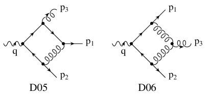
FIG. 2.: NLO box contributions to the three-jet decay rate of the $Z$-boson into massive quarks.

Both four-point functions are IR divergent. The integral $D05$ has a simple infrared pole, while $D06$ presents double infrared poles because it involves a three-gluon vertex. Before the calculation of these integrals we would like to discuss their IR behavior. To do that we just need to split their non on-shell propagator.

For the $D05$ integral we have

$$\frac{1}{(k+p_{13})^{2}-m_{b}^{2}} = \frac{1}{p_{13}^{2}-m_{b}^{2}}$$ (28)

$$- \frac{k^{2}+2k\cdot p_{13}}{(p_{13}^{2}-m_{b}^{2})[(k+p_{13})^{2}-m_{b}^{2}]}~{}.$$ (29)

The infrared divergence is isolated in the first term of the righthand side of the previous equation that give rise to $C05(y_{12})/y_{13}$, where $C05$ is the three-point function defined in eq. (20). The other term generates two infrared finite one-loop integrals.

For the $D06$ function things are quite more complex. The splitting of the non on-shell propagator does not give directly the divergent piece due to the presence of double infrared poles. First of all, we have to notice that $D06$ is invariant under the interchange of particles 1 and 2, i.e., the result of the integral should be symmetric in the two-momenta invariants $y_{13}$ and $y_{23}$. The proper way for extracting the infrared piece is as follows [14]

$$D06(y_{13},y_{23}) = \frac{1}{y_{13}}C03(y_{23})$$ (30)

$$+ \frac{1}{y_{23}}C03(y_{13})+\mathrm{finite\,terms}~{}.$$ (31)

The box integral, $D05$, comes from an electroweak-like Feynman diagram and it has already been calculated [15] by using a photon mass infrared regulator. Since only simple infrared poles appear in the $D05$ function, we are allowed to identify the logarithm of the gluon (photon) mass, $\log\lambda^{2}$, in the result of ref. [15], with a pole in dimensional regularization: $\log\lambda^{2}\rightarrow(4\pi)^{\epsilon}/\Gamma(1-\epsilon)/\epsilon$. Thus, we have

$$D05(y_{13},y_{12}) = s^{-2-\epsilon}\mu^{2\epsilon}\frac{(4\pi)^{\epsilon}}{\Gamma(1-\epsilon)}\frac{1}{(y_{12}+2r_{b})\beta_{12}y_{13}}$$ (32)

$$\times \bigg{[}\left(\frac{1}{\epsilon}-\log\frac{r_{b}}{y_{13}^{2}}\right)\log c_{12}$$ (33)

$$+ \pi^{2}+\log^{2}c-Li_{2}(1-c_{12}^{2})$$ (34)

$$+ 2Li_{2}(1-c_{12}~{}c)+2Li_{2}(1-c_{12}/c)\bigg{]}~{},$$ (35)

with

$$\beta=\sqrt{1-4r_{b}}~{},\qquad c=\frac{1-\beta}{1+\beta}~{}.$$ (36)

To calculate $D06$ we consider the following set of Feynman parametrizations

$$\frac{1}{k^{2}(k+p_{3})^{2}}=\int_{0}^{1}\frac{dz}{[k^{2}+2k\cdot p_{3}z]^{2}}~{},$$ (37)

$$\frac{1}{[(k+p_{13})^{2}-m_{b}^{2}][(k-p_{2})^{2}-m_{b}^{2}]}=$$ (38)

$$\qquad\int_{0}^{1}\frac{dy}{[k^{2}+(2k\cdot q+2p_{1}\cdot p_{3})y-2k\cdot p_{2}]^{2}}~{},$$ (39)

that again we combine with the help of the identity

$$\frac{1}{a^{2}b^{2}}=\int_{0}^{1}dx\frac{6x(1-x)}{[a\,x+b(1-x)]^{4}}~{}.$$ (40)

After these parametrizations our integral becomes linear in the $z$-Feynman parameter

$$\frac{i}{16\pi^{2}}D06(y_{13},y_{23})=\mu^{4-D}\int_{0}^{1}6x(1-x)dx\,dy$$ (41)

$$\times\int\frac{d^{D}k}{(2\pi)^{D}}\int_{0}^{1}\frac{dz}{[k^{2}-(M_{1}z+M_{0}(1-z))+i\eta]^{4}}~{},$$ (42)

where we defined

$$M_{0} = s\,(1-x)\left[r_{b}\,(1-x)-(1-x)\,y(1-y)-y_{13}xy\right]~{},$$ (43)

$$M_{1} = s\,(1-x)\left[r_{b}\,(1-x)-(1-x)\,y(1-y)-y_{23}x(1-y)\right]~{}.$$ (44)

Again we will omit the $i\eta$ term, and, when needed, we will use the prescription $r_{b}\rightarrow r_{b}-i\eta$, $y_{13,23}\rightarrow y_{13,23}+i\eta$.

Performing the $z$-integration before the integration over the loop momentum we obtain

$$\frac{i}{16\pi^{2}}D06(y_{13},y_{23})=s^{-1}\mu^{2\epsilon}\int_{0}^{1}\frac{2dx\,dy}{y_{13}y-y_{23}(1-y)}$$ (45)

$$\times\int\frac{d^{D}k}{(2\pi)^{D}}\left\{\frac{1}{(k^{2}-M_{1})^{3}}-\frac{1}{(k^{2}-M_{0})^{3}}\right\}~{},$$ (46)

that results, after integration over the loop momentum, into

$$D06(y_{13},y_{23})=s^{-2-\epsilon}\mu^{2\epsilon}(4\pi)^{\epsilon}\Gamma(1+\epsilon)$$ (47)

$$\times\int_{0}^{1}\frac{dy~{}A^{-1-\epsilon}}{y_{13}y-y_{23}(1-y)}\int_{0}^{1}d\,x\ (1-x)^{-1-\epsilon}\left[1-x(1+\frac{y_{13}y}{A})\right]^{-1-\epsilon}$$ (48)

$$\qquad\qquad\qquad\qquad\qquad\qquad\qquad+(y_{13}\leftrightarrow y_{23})~{},$$ (49)

where

$$A=r_{b}-y(1-y)~{}.$$ (50)

After integration over the $x$-Feynman parameter we get a hypergeometric function

$$D06(y_{13},y_{23})=s^{-2-\epsilon}\mu^{2\epsilon}(4\pi)^{\epsilon}\frac{\Gamma(1+\epsilon)}{-\epsilon}$$ (51)

$$\times\int_{0}^{1}dy\frac{A^{-1-\epsilon}}{y_{13}y-y_{23}(1-y)}\ {}_{2}F_{1}[1+\epsilon,1;1-\epsilon;1+\frac{y_{13}y}{A}]$$ (52)

$$\qquad\qquad\qquad\qquad\qquad\qquad\qquad+(y_{13}\leftrightarrow y_{23})~{}.$$ (53)

Again, using the transformation properties of ${}_{2}F_{1}$ and expanding in $\epsilon$, we can write the above hypergeometric function in terms of the dilogarithm function, see appendix A. Moreover, as the dilogarithm function contributes at the order $O(\epsilon^{2})$ we are allowed to substitute it with its value at $y=0$, $Li_{2}(1)=\pi^{2}/6$, obtaining

$$D06(y_{13},y_{23})=s^{-2-\epsilon}\mu^{2\epsilon}(4\pi)^{\epsilon}\frac{\Gamma(1+\epsilon)}{-\epsilon}(1+\epsilon^{2}\frac{\pi^{2}}{3})$$ (54)

$$\times\left(\int_{0}^{1}dy\frac{(-y_{13}y)^{-1-2\epsilon}}{y_{13}y-y_{23}(1-y)}A^{\epsilon}+(y_{13}\leftrightarrow y_{23})~{}\right).$$ (55)

Partly expanding in $\epsilon$ to the required order, we can rewrite our integral before the last integration in the following form

$$D06(y_{13},y_{23})=s^{-2-\epsilon}\mu^{2\epsilon}\frac{(4\pi r_{b})^{\epsilon}}{\Gamma(1-\epsilon)}\frac{-1}{\epsilon}(1+\epsilon^{2}\frac{\pi^{2}}{2})$$ (56)

$$\times\int_{0}^{1}dy\left(\frac{(-y_{13}y)^{-1-2\epsilon}}{y_{13}y-y_{23}(1-y)}-\epsilon\frac{\log(1-y(1-y)/r_{b})}{y_{13}y(y_{13}y-y_{23}(1-y))}\right)$$ (57)

$$\qquad\qquad\qquad\qquad\qquad\qquad\qquad\qquad\qquad+(y_{13}\leftrightarrow y_{23})~{},$$ (58)

where we have used $\Gamma(1+\epsilon)\Gamma(1-\epsilon)=(1+\epsilon^{2}\pi^{2}/6+O(\epsilon^{4}))$. The first part of the integrand gives, up to a factor $-(-y_{13})^{-2\epsilon}/y_{13}/y_{23}/(-2\epsilon)$ a hypergeometric function that can be reduced to the dilogarithm,

$${}_{2}F_{1}[1,-2\epsilon;1-2\epsilon;\frac{y_{13}+y_{23}}{y_{23}}]=$$ (59)

$$\qquad\left(-\frac{y_{13}}{y_{23}}\right)^{2\epsilon}\left[1+4\epsilon^{2}Li_{2}\left(\frac{y_{13}+y_{23}}{y_{13}}\right)+O(\epsilon^{3})\right]~{}.$$ (60)

Using the above equation and the symmetry $y_{13}\leftrightarrow y_{23}$, we can rewrite $D06(y_{13},y_{23})$  as

$$D06(y_{13},y_{23})=s^{-2-\epsilon}\mu^{2\epsilon}\frac{(4\pi r_{b})^{\epsilon}}{\Gamma(1-\epsilon)}(1+\epsilon^{2}\frac{\pi^{2}}{2})\frac{1}{y_{13}y_{23}2\epsilon^{2}}$$ (61)

$$\bigg{[}(-y_{13})^{-2\epsilon}\left(\frac{-y_{23}}{y_{13}}\right)^{-2\epsilon}+(-y_{23})^{-2\epsilon}\left(\frac{-y_{23}}{y_{13}}\right)^{2\epsilon}+$$ (62)

$$2\epsilon^{2}\left(2Li_{2}\left(\frac{y_{13}+y_{23}}{y_{23}}\right)+2Li_{2}\left(\frac{y_{13}+y_{23}}{y_{13}}\right)-\int_{0}^{1}dy\frac{\log(1-y(1-y)/r_{b})}{y(1-y)}\right)\left.\right.\bigg{]}~{}.$$ (63)

Performing the last integral, and fully expanding in $\epsilon$ (in this expansion the $i\eta$ prescription should be used to avoid ambiguities) we have the following final result for the real part of the function $D06(y_{13},y_{23})$

$$D06(y_{13},y_{23}) = s^{-2-\epsilon}\mu^{2\epsilon}\frac{(4\pi)^{\epsilon}}{\Gamma(1-\epsilon)}\frac{1}{y_{13}y_{23}}$$ (64)

$$\times \left[\frac{1}{\epsilon^{2}}+\frac{1}{\epsilon}\log\frac{r_{b}}{y_{13}y_{23}}\right.$$ (65)

$$- \left.\log^{2}c+\frac{1}{2}\log\frac{r_{b}}{y_{13}^{2}}\log\frac{r_{b}}{y_{23}^{2}}-\frac{3\pi^{2}}{2}\right]~{}.$$ (66)

III Infrared divergent phase-space integrals

We consider now the tree-level four-parton decay $q\rightarrow p_{1}+p_{2}+p_{3}+p_{4}$. When at least one gluon is radiated from an external quark (or gluon) line, the propagator-factors, $1/(p_{i}\cdot p_{j})$, can generate infrared and gluon-gluon collinear divergences at the border of the four-body phase-space. In this section we integrate these factors in a thin slice at the border of the phase-space and we show how these basic phase-space integrals are related to the infrared divergent scalar one-loop integrals of the previous section.

A Integrals containing soft gluon divergences

The phase-space of $n+1$ particles can be written as the product of the $n$-body phase-space times the integral over the energy and the solid angle of the extra particle. In arbitrary $D=4-2\epsilon$ dimensions we have

$$dPS(n+1)=\frac{1}{2(2\pi)^{D-1}}E^{D-3}\>dE\>d\Omega\>dPS(n)~{}.$$ (67)

Suppose $E_{3}$ is the energy of a soft gluon: $E_{3}<w$ where $w$, with $w$ very small, is an upper cut on the soft gluon energy. Let’s consider

$$\int_{0}^{w}E_{3}^{D-3}dE_{3}\>d\Omega\frac{1}{(2p_{1}\cdot p_{3})^{2}}~{},$$ (68)

where $p_{3}$ is the momentum of the gluon and $p_{1}$ is the momentum of a quark. After integration over the trivial angles we find ($x=\cos\theta$, with $\theta$ being the angle between $\vec{p_{1}}$ and $\vec{p_{3}}$)

$$\frac{2\pi^{\frac{D}{2}-1}}{4\Gamma\left(\frac{D}{2}-1\right)}\int_{0}^{w}dE_{3}E_{3}^{D-5}\int_{-1}^{1}dx\frac{(1-x^{2})^{\frac{D-4}{2}}}{(E_{1}-{\bf p}_{1}x)^{2}}~{}.$$ (69)

Here ${\bf p}_{1}$ stands for the modulus of the threemomentum. In the eikonal region we can suppose $E_{1}$ being almost independent from $E_{3}$

$$E_{1}\simeq\frac{\sqrt{s}}{2}(1-y_{24})~{},$$ (70)

with $y_{24}=2(p_{2}\cdot p_{4})/s$. The integral over $E_{3}$ can be easily done and gives a simple infrared pole in $\epsilon$. Since the $x$ dependent part is completely finite we can expand in $\epsilon$ before the integral over this variable is performed. The final result we get is as follows

$$\frac{1}{2(2\pi)^{D-1}} \int_{0}^{w}E_{3}^{D-3}dE_{3}d\Omega\frac{1}{(2p_{1}\cdot p_{3})^{2}}=$$ (73)

$$\frac{1}{16\pi^{2}}\frac{(4\pi)^{\epsilon}}{\Gamma(1-\epsilon)}\frac{1}{E_{1}^{2}-{\bf p}_{1}^{2}}$$

$$\times\left[-\frac{1}{2\epsilon}+\log 2\omega+\frac{E_{1}}{2{\bf p}_{1}}\log\frac{E_{1}-{\bf p}_{1}}{E_{1}+{\bf p}_{1}}\right]~{}.$$

Let’s consider now

$$\int_{0}^{w}E_{3}^{D-3}dE_{3}d\Omega\frac{1}{(2p_{1}\cdot p_{3})(2p_{2}\cdot p_{3})}~{},$$ (74)

with $p_{2}$ the momentum of the antiquark. In this case we can combine the denominators as follows

$$\frac{1}{(2p_{1}\cdot p_{3})(2p_{2}\cdot p_{3})}=\int_{0}^{1}dy\frac{1}{[2p_{3}\cdot(p_{1}+(p_{2}-p_{1})y)]^{2}}~{}.$$ (75)

We get therefore the same integral structure as in eq. (73), but with the fourmomentum $p_{A}=p_{1}+(p_{2}-p_{1})y$, instead of $p_{1}$. After integration over the y-parameter we get

$$\frac{1}{2(2\pi)^{D-1}} \int_{0}^{w}E_{3}^{D-3}dE_{3}d\Omega\frac{1}{(2p_{1}\cdot p_{3})(2p_{2}\cdot p_{3})}=$$ (78)

$$\frac{1}{16\pi^{2}}\frac{(4\pi)^{\epsilon}}{\Gamma(1-\epsilon)}\left[\left(\frac{1}{2\epsilon}-\log 2\omega\right)\right.$$

$$\times\left.\frac{2}{(y_{12}+2r_{b})\beta_{12}}\log c_{12}+F(y_{14},y_{24})\right]~{}.$$

Notice that this last integral has the same divergent structure as the scalar one loop $C05$ function defined in eq. (20). The finite contribution, the $F(y_{14},y_{24})$ function, is rather involved. We write it in terms of the variables $y_{13}$ and $y_{23}$ for later convenience

$$F(y_{13},y_{23})=\frac{1}{b\sqrt{1-a^{2}}}[G(z_{1})+G(z_{2})-2G(1)]~{},$$ (79)

where

$$G(z)=\log t_{1}\log\frac{t_{1}-z}{t_{1}+z}+\log t_{2}\log\frac{z+t_{2}}{z-t_{2}}$$ (80)

$$+ \log\frac{t_{1}-t_{2}}{2}\log\frac{(t_{1}+z)(z-t_{2})}{(t_{1}-z)(z+t_{2})}$$ (81)

$$+ \frac{1}{2}\left[\log^{2}(t_{1}+z)+\log^{2}(t_{1}-z)\right.$$ (82)

$$+ \left.\log^{2}(z-t_{2})-\log^{2}(z+t_{2})\right]$$ (83)

$$- \frac{1}{4}\left[\log(t_{1}+z)+\log(t_{1}-z)+\log\left(\frac{z-t_{2}}{z+t_{2}}\right)\right]^{2}$$ (84)

$$+ Li_{2}\left(\frac{z-t_{2}}{z-t_{1}}\right)+Li_{2}\left(\frac{z-t_{1}}{z+t_{1}}\right)$$ (85)

$$- Li_{2}\left(\frac{z+t_{2}}{z+t_{1}}\right)-Li_{2}\left(\frac{z-t_{2}}{z+t_{2}}\right)~{},$$ (86)

with

$$a=\sqrt{h_{p}}/b~{},$$ (87)

$$b^{2}=1-4r_{b}-2(1-2r_{b})(y_{13}+y_{23})$$ (88)

$$\qquad+(1-r_{b})(y_{13}^{2}+y_{23}^{2})+y_{13}y_{23}(3-2r_{b}-y_{13}-y_{23})~{},$$ (89)

where $h_{p}$ is the function that defines the limits of the three-body phase-space, see eq. (B6), and

$$t_{1,2}=(1\pm\sqrt{1-a^{2}})/a~{},$$ (90)

$$z_{1}=\exp\left[\cosh^{-1}\left(\sqrt{(1-y_{13})^{2}-4r_{b}}/(a(1-y_{13}))\right)\right]~{},$$ (91)

$$z_{2}=\exp\left[\cosh^{-1}\left(\sqrt{(1-y_{23})^{2}-4r_{b}}/(a(1-y_{23}))\right)\right]~{}.$$ (92)

B Integrals containing gluon-gluon collinear divergences

Let’s consider the following phase-space integral

$$PS(4)\frac{1}{y_{13}y_{34}}~{}.$$ (93)

We work in the so-called “3-4 system”, eq. (B20), where as usual $p_{1}$ denotes the momentum of the quark and $p_{3}$ and $p_{4}$ are the two gluon momenta. This integral has a singularity when either the gluon labeled as “3” is soft or the two gluons are collinear, that is $y_{34}=0$. Then we take $y_{34}<w$ with $w$ very small. We can decompose the four-body phase-space as the product of a three-body phase-space in terms of variables $y_{134}$ and $y_{234}$ times the integral over $y_{34}$ and the two angular variables $v$ and $\theta^{\prime}$

$$PS(4) \frac{1}{y_{13}y_{34}}=PS(3)(y_{134},y_{234})$$ (96)

$$\times\frac{S}{16\pi^{2}}\frac{(4\pi)^{\epsilon}}{\Gamma(1-\epsilon)}\frac{1}{N_{\theta^{\prime}}}\int_{0}^{\pi}d\theta^{\prime}\sin^{-2\epsilon}\theta^{\prime}$$

$$\times\int_{0}^{1}dv(v(1-v))^{-\epsilon}\int_{0}^{w}dy_{34}\frac{y_{34}^{-1-\epsilon}}{y_{13}}~{},$$

where $S=1/2!$ is the statistical factor. In the “3-4 system” the two-momenta invariant $y_{13}$ can be written in terms of the integration variables as

$$y_{13}=\frac{1}{2}\left(y_{134}-\sqrt{y_{134}^{2}-4r_{b}y_{34}}(1-2v)\right)~{}.$$ (97)

The $y_{13}$ factor is independent of the $\theta^{\prime}$-angle so we can get rid of this first integral. Moreover, $y_{13}$ contains a piece independent of the $v$-variable and another one that is odd under the interchange $v\leftrightarrow(1-v)$. With the help of this symmetry we can avoid the use of the square root in eq. (97) by using the identity

$$\frac{1}{2}\left(\frac{1}{g+f(v)}+\frac{1}{g-f(v)}\right)=\frac{g}{g^{2}-f(v)^{2}}~{},$$ (98)

then, we rewrite our integral as

$$PS(4)\frac{1}{y_{13}y_{34}}=PS(3)(y_{134},y_{234})$$ (99)

$$\times\frac{S}{16\pi^{2}}\frac{(4\pi)^{\epsilon}}{\Gamma(1-\epsilon)}\int_{0}^{1}dv(v(1-v))^{-\epsilon}\int_{0}^{w}y_{34}^{-1-\epsilon}dy_{34}$$ (100)

$$\times\frac{2y_{134}}{y_{134}^{2}-(y_{134}^{2}-4r_{b}y_{34})(1-2v)^{2}}~{}.$$ (101)

After integration over $y_{34}$ we get the first infrared pole

$$PS(4)\frac{1}{y_{13}y_{34}} = PS(3)\frac{S}{16\pi^{2}}\frac{(4\pi)^{\epsilon}}{\Gamma(1-\epsilon)}\frac{-1}{\epsilon}\frac{w^{-\epsilon}}{2y_{134}}$$ (102)

$$\times \int_{0}^{1}dv(v(1-v))^{-1-\epsilon}{}_{2}F_{1}[1,-\epsilon;1-\epsilon;-B\frac{(1-2v)^{2}}{v(1-v)}]~{},$$ (103)

with $B=w(r_{b}/y_{134}^{2})$. Similarly to eq. (60) we can write ${}_{2}F_{1}$ in terms of a dilogarithm function

$${}_{2}F_{1} [1,-\epsilon;1-\epsilon;-\frac{a}{b}]=$$ (105)

$$\left(\frac{b}{a+b}\right)^{-\epsilon}\left[1+\epsilon^{2}Li_{2}\left(\frac{a}{a+b}\right)+O(\epsilon^{3})\right]~{}.$$

Thus, we obtain

$$PS(4)\frac{1}{y_{13}y_{34}} = PS(3)\frac{S}{16\pi^{2}}\frac{(4\pi)^{\epsilon}}{\Gamma(1-\epsilon)}\frac{-1}{\epsilon}\frac{w^{-\epsilon}}{2y_{134}}\int_{0}^{1}dv(v(1-v))^{-1-2\epsilon}$$ (106)

$$\times \left(v(1-v)+B(1-2v)^{2}\right)^{\epsilon}$$ (107)

$$\times \left[1+\epsilon^{2}Li_{2}\left(\frac{B(1-2v)^{2}}{v(1-v)+B(1-2v)^{2}}\right)+O(\epsilon^{3})\right]~{}.$$ (108)

The above integrand is symmetric under the interchange $v\leftrightarrow(1-v)$. We perform the integral only in half of the integration region and apply the following change of variables

$$u=4v(1-v)~{}.$$ (109)

In addition, since the IR divergence occurs at $u=0$ and the term proportional to the dilogarithm function is already order $\epsilon^{2}$, we can substitute the dilogarithm function by its value at $u=0$, that is $Li_{2}(1)=\pi^{2}/6$. After this, we get

$$PS(4)\frac{1}{y_{13}y_{34}} = PS(3)\frac{S}{16\pi^{2}}\frac{(4\pi)^{\epsilon}}{\Gamma(1-\epsilon)}\frac{-1}{\epsilon}\frac{w^{-\epsilon}B^{\epsilon}}{y_{134}}2^{4\epsilon}\left(1+\epsilon^{2}\frac{\pi^{2}}{6}\right)$$ (110)

$$\times \int_{0}^{1}du\,u^{-1-2\epsilon}(1-u)^{-1/2}\left[1-\left(1-\frac{1}{4B}\right)u\right]^{\epsilon}~{},$$ (111)

which gives again a hypergeometric function

$$PS(4)\frac{1}{y_{13}y_{34}} = PS(3)\frac{S}{16\pi^{2}}\frac{(4\pi)^{\epsilon}}{\Gamma(1-\epsilon)}\frac{-1}{\epsilon}\frac{1}{y_{134}}\left(\frac{r_{b}}{y_{134}^{2}}\right)^{\epsilon}2^{4\epsilon}\left(1+\epsilon^{2}\frac{\pi^{2}}{6}\right)\sqrt{\pi}$$ (112)

$$\times \frac{\Gamma(-2\epsilon)}{\Gamma(\frac{1}{2}-2\epsilon)}{}_{2}F_{1}[-\epsilon,-2\epsilon;\frac{1}{2}-2\epsilon;1-\frac{1}{4B}]~{}.$$ (113)

The hypergeometric function is already $1+O(\epsilon^{2})$ but now it is not possible to write it in terms of a dilogarithm function. If we are interested just in the pole structure we can stop here. (Observe that neither the double pole or the simple one depend on the eikonal cut $w$). To get the complete finite part further mathematical manipulations must be performed with the hypergeometric function. We use [16]

$${}_{2}F_{1} [-\epsilon,-2\epsilon;\frac{1}{2}-2\epsilon;1-\frac{1}{4B}]=$$ (117)

$$(4B)^{2\epsilon}\Gamma(\frac{1}{2}-2\epsilon)$$

$$\times\left\{\frac{\Gamma(\epsilon)}{\Gamma(-\epsilon)\Gamma(\frac{1}{2})}{}_{2}F_{1}[-2\epsilon,\frac{1}{2}-\epsilon;1-\epsilon;4B]\right.$$

$$+\left.\frac{\Gamma(-\epsilon)}{\Gamma(-2\epsilon)\Gamma(\frac{1}{2}-\epsilon)}{}_{2}F_{1}[-\epsilon,\frac{1}{2};1+\epsilon;4B]\right\}~{}.$$

For $w$ small enough, $w\ll y_{134}^{2}/r_{b}$, we can use the Gauss series [16] to expand the hypergeometric functions around $B\rightarrow 0$. The final result we obtain is as follows

$$dPS(4)\frac{1}{y_{13}y_{34}}=dPS(3)(y_{134},y_{234})\frac{S}{16\pi^{2}}\frac{(4\pi)^{\epsilon}}{\Gamma(1-\epsilon)}\frac{1}{y_{134}}$$ (118)

$$\times\left\{\frac{1}{2\epsilon^{2}}-\frac{1}{2}\log^{2}w+\left(\frac{1}{2\epsilon}-\log w\right)\log\frac{r_{b}}{y_{134}^{2}}\right.-\frac{1}{4}\log^{2}\frac{r_{b}}{y_{134}^{2}}-\frac{\pi^{2}}{4}+O(w)\biggr{\}}~{}.$$ (119)

Notice we get the same infrared poles as in the one-loop three point function $C03$, eq. (18), if we identify $y_{134}$ with $y_{13}$. In the limit $y_{34}\rightarrow 0$ the momentum $p_{34}=p_{3}+p_{4}$ behaves as the momentum of a pseudo on-shell massless particle since $p_{34}^{2}\rightarrow 0$ and the function that defines the limits of the four-body phase-space, $h_{34}$ in eq. (B25), reduces to the three-body phase-space function $h_{p}$, see eq. (B6). Therefore, within this limit, this identification provides the key to see the cancellation of the infrared divergences.

IV Summary

We have presented the basic ingredients needed to compute the second order QCD corrections to the three-jet decay rate of the $Z$-boson into massive quarks. This includes, for massive quarks, the first calculation of the double infrared divergent box integral, we called $D06$, in dimensional regularization. We have presented results for both the infrared part and the finite contributions of some basic infrared divergent one-loop and phase-space integrals. We showed they share the same infrared behavior. Therefore, the cancellation of the infrared divergences is assured as stated by the BN and KLN theorems [4].

We would like to acknowledge interesting discussions with S. Catani, A. Denner, A. Manohar and A. Pich. We are also indebted with S. Cabrera, J. Fuster and S. Martí for an enjoyable collaboration. M.B. thanks the Univ. de València for the warm hospitality during his visit. The work of G.R. and A.S. has been supported in part by CICYT (Spain) under the grant AEN-96-1718 and IVEI. The work of G.R. has also been supported in part by CSIC-Fundació Bancaixa.

A Some properties of the hypergeometric function

Here we present some properties of the hypergeometric function [16] we use in the main body of the paper. The integral representation of the hypergeometric function is

$${}_{2}F_{1}[a,b;c;z]=\frac{\Gamma(c)}{\Gamma(b)\Gamma(c-b)}\int_{0}^{1}d\,t\ t^{b-1}(1-t)^{c-b-1}(1-tz)^{-a}~{}.$$ (A1)

From the above equation one can derive the following transformation properties,

$${}_{2}F_{1}[a,b;c;z] = (1-z)^{c-a-b}{}_{2}F_{1}[c-a,c-b;c;z]$$ (A2)

$$= (1-z)^{-b}{}_{2}F_{1}[b,c-a;c;\frac{z}{z-1}]~{}.$$ (A3)

Using the Gauss series for the hypergeometric function [16] one can easily see that

$${}_{2}F_{1}[\alpha\epsilon,\beta\epsilon;1+\gamma\epsilon;z]=1+\epsilon^{2}\alpha\beta Li_{2}(z)+O(\epsilon^{3})~{},$$ (A4)

where, $Li_{2}(z)$ is the Spence or dilogarithm function

$$Li_{2}(z)=-\int_{0}^{z}dt\frac{\log(1-t)}{t}~{}.$$ (A5)

B phase-space in $D=4-2\epsilon$ dimensions

The phase-space for $n$-particles in the final state in arbitrary $D$ space-time dimensions [5] $(D=4-2\epsilon)$ has the following general form

$$dPS(n) = (2\pi)^{D}\prod_{i=1,n}\frac{d^{D-1}p_{i}}{(2\pi)^{D-1}2E_{i}}\delta^{D}\left(q-\sum_{i=1,n}p_{i}\right)$$ (B1)

$$= (2\pi)^{D}\prod_{i=1,n}\frac{d^{D}p_{i}}{(2\pi)^{D-1}}$$ (B2)

$$\times \delta(p_{i}^{2}-m_{i}^{2})\Theta(E_{i})\delta^{D}\left(q-\sum_{i=1,n}p_{i}\right)~{}.$$ (B3)

Let’s consider the decay into three particles, $q\rightarrow p_{1}+p_{2}+p_{3}$, where particles 1 and 2 share the same mass, $p_{1}^{2}=p_{2}^{2}=m_{b}^{2}$, and particle 3 is massless, $p_{3}^{2}=0$. In terms of the two-momenta invariant variables $y_{13}=2(p_{1}\cdot p_{3})/s$ and $y_{23}=2(p_{2}\cdot p_{3})/s$, with $s=q^{2}$, we get

$$PS(3) = \frac{s}{16(2\pi)^{3}}\frac{1}{\Gamma(2-2\epsilon)}{\left(\frac{s}{4\pi}\right)}^{-2\epsilon}$$ (B4)

$$\times \int\theta(h_{p})h_{p}^{-\epsilon}dy_{13}dy_{23}~{},$$ (B5)

where the function $h_{p}$ which gives the phase-space boundary has the form

$$h_{p}=y_{13}y_{23}(1-y_{13}-y_{23})-r_{b}(y_{13}+y_{23})^{2}~{},$$ (B6)

with $r_{b}=m_{b}^{2}/s$.

For the case of the decay into two massive and two massless particles, $q\rightarrow p_{1}+p_{2}+p_{3}+p_{4}$ with $p_{1}^{2}=p_{2}^{2}=m_{b}^{2}$ and $p_{3}^{2}=p_{4}^{2}=0$, it is convenient to write the four-body phase-space as a quasi three-body decay

$$\qquad\qquad q\rightarrow p_{34}+p_{1}+p_{2}$$ (B8)

$$\hookrightarrow p_{3}+p_{4}~{}.$$

In the c.m. frame of particles 3 and 4 the four-momenta can be written as

$$p_{1} = (E_{1},\ldots,0,{\bf p}_{1})~{},$$ (B9)

$$p_{2} = (E_{2},\ldots,{\bf p}_{2}\sin\beta,{\bf p}_{2}\cos\beta)~{},$$ (B10)

$$p_{3} = E_{3}(1,\ldots,\sin\theta\cos\theta^{\prime},\cos\theta)~{},$$ (B11)

$$p_{4} = E_{4}(1,\ldots,-\sin\theta\cos\theta^{\prime},-\cos\theta)~{},$$ (B12)

where the dots in $p_{3}$ and $p_{4}$ indicate $D-3$ unspecified, equal and opposite angles (in $D$ dimensions) and $D-3$ zeros in $p_{1}$ and $p_{2}$. We will refer to this as the “3-4 system” [7].

Energies and threemomenta can be written in terms of the following invariants

$$y_{34}=\frac{2(p_{3}\cdot p_{4})}{s}~{},$$ (B13)

$$y_{134}=\frac{2(p_{1}\cdot p_{34})}{s}~{},\qquad y_{234}=\frac{2(p_{2}\cdot p_{34})}{s}~{},$$ (B14)

where $p_{34}=p_{3}+p_{4}$. We obtain

$$E_{1} = \frac{y_{134}\sqrt{s}}{2\sqrt{y_{34}}}~{},\qquad{\bf p}_{1}=\frac{\sqrt{s}}{2\sqrt{y_{34}}}\sqrt{y_{134}^{2}-4r_{b}y_{34}}~{},$$ (B15)

$$E_{2} = \frac{y_{234}\sqrt{s}}{2\sqrt{y_{34}}}~{},\qquad{\bf p}_{2}=\frac{\sqrt{s}}{2\sqrt{y_{34}}}\sqrt{y_{234}^{2}-4r_{b}y_{34}}~{},$$ (B16)

$$E_{3} = E_{4}=\frac{\sqrt{y_{34}\,s}}{2}~{}.$$ (B17)

Setting $v=(1-\cos\theta)/2$, the $D$-dimensional phase-space in this system is

$$PS(4)=\frac{s}{16(2\pi)^{3}}\frac{1}{\Gamma(2-2\epsilon)}{\left(\frac{s}{4\pi}\right)}^{-2\epsilon}\int dy_{134}dy_{234}$$ (B18)

$$\times s^{1-\epsilon}\frac{S}{16\pi^{2}}\frac{(4\pi)^{\epsilon}}{\Gamma(1-\epsilon)}\int dy_{34}\theta(h_{34})h_{34}^{-\epsilon}y_{34}^{-\epsilon}$$ (B19)

$$\times\int_{0}^{1}dv(v(1-v))^{-\epsilon}\frac{1}{N_{\theta^{\prime}}}\int_{0}^{\pi}d\theta^{\prime}\sin^{-2\epsilon}\theta^{\prime}~{},$$ (B20)

where $S=1/2!$ is the statistical factor, $N_{\theta^{\prime}}$ is a normalization factor

$$N_{\theta^{\prime}}=\int_{0}^{\pi}d\theta^{\prime}\sin^{-2\epsilon}\theta^{\prime}=2^{2\epsilon}\pi\frac{\Gamma(1-2\epsilon)}{\Gamma^{2}(1-\epsilon)}~{},$$ (B21)

and the function

$$h_{34} = y_{134}y_{234}(1-y_{134}-y_{234})-r_{b}(y_{134}+y_{234})^{2}$$ (B22)

$$+ \left(-1+4r_{b}+2(1-2r_{b})(y_{134}+y_{234})\right.$$ (B23)

$$- \left.y_{134}^{2}-3y_{134}y_{234}-y_{234}^{2}\right)y_{34}$$ (B24)

$$+ 2(1-2r_{b}-y_{134}-y_{234})y_{34}^{2}-y_{34}^{3}~{},$$ (B25)

defines the limits of the phase-space. Observe that $h_{34}$ reduces to eq. (B6) in the case $y_{34}\rightarrow 0$. Furthermore, in this limit, $p_{34}=p_{3}+p_{4}$ behaves as the momentum of a pseudo on-shell massless particle since $p_{34}^{2}\rightarrow 0$.

REFERENCES

• [1] M. Bilenky, G. Rodrigo and A. Santamaria, Nucl. Phys. B439, 505 (1995).
• [2] J. Fuster, Recent results on QCD at LEP, Proc. XXII International Meeting on Fundamental Physics, Jaca, Spain, 1994; J. Fuster, S. Cabrera and S. Martí, Experimental studies of QCD using flavour tagged jets with DELPHI, Proceedings of the High-energy Physics International Euroconference on Quantum Chromodynamics (QCD 96), Montpellier, France, 4-12 Jul, 1996, hep-ex/9609004; J. Fuster, Tests of QCD at LEP, XXV international meeting on fundamental physics. Formigal – Huesca, Spain. March 3 – 8, 1997.
• [3] G. Rodrigo, Quark mass effects in QCD jets, Proceedings of the High-energy Physics International Euroconference on Quantum Chromodynamics (QCD 96), Montpellier, France, 4-12 Jul, 1996, hep-ph/9609213; G. Rodrigo, Quark mass effects in QCD jets, PhD thesis, Universitat de València, 1996, hep-ph/9703359, ISBN: 84-370-2989-9; G. Rodrigo, A. Santamaria and M. Bilenky, Do the quark masses run? Extracting $\bar{m}_{b}(m_{Z})$ from LEP data, hep-ph/9703358.
• [4] F. Bloch and A. Nordsieck, Phys. Rev. 52 (1937) 54; T. Kinoshita, J. Math. Phys. 3(1962)650; T.D. Lee and M. Nauenberg, Phys. Rev. B133 (1964) 1549.
• [5] R. Gastmans and R. Meudermans, Nucl. Phys. B63, 277 (1973); W.J. Marciano and A. Sirlin, Nucl. Phys. B88, 86 (1975); W.J. Marciano, Phys. Rev. D12, 3861 (1975).
• [6] W.T. Giele, S. Keller and E. Laenen, Phys. Lett. B372, 141 (1996); W.T. Giele, E.W.N. Glover and D.A. Kosower, Nucl. Phys. B403, 633 (1993); W.T. Giele and E.W.N. Glover, Phys. Rev. D46, 1980 (1992); F. Aversa, M. Greco, P. Chiappetta and J.P. Guillet, Phys. Rev. Lett. 65, 90 (19401); H. Baer, J. Ohnemus and J.F. Owens, Phys. Rev. DD40, 2844 (1989); F. Gutbrod, G. Kramer and G. Schierholz, Zeit. Phys. C21, 235 (1984).
• [7] R.K. Ellis, D.A. Ross and A.E. Terrano, Nucl. Phys. B178, 421 (1981).
• [8] Z. Kunszt and P. Nason, in ‘Z Physics at LEP 1’, CERN 89-08, vol. 1, p. 373; S. Bethke, Z. Kunszt, D.E. Soper and W.J. Stirling, Nucl. Phys. B370, 310 (1992).
• [9] S. Catani and M.H. Seymour, Nucl. Phys. B485, 291 (1997), Phys. Lett. B378, 287 (1996); S. Frixione, Z. Kunszt and A. Signer, Nucl. Phys. B467, 399 (1996); Z. Kunszt and D.E. Soper, Phys. Rev. D46, 192 (1992); M.L. Mangano, P. Nason and G. Ridolfi, Nucl. Phys. B373, 295 (1992); S.D. Ellis, Z. Kunszt and D.E. Soper, Phys. Rev. D40, 2188 (1989).
• [10] K. Fabricius and I. Schmitt, Zeit. Phys. C3, 51 (1979); S. Papadopoulos, A.P. Contogouris and J. Ralston Phys. Rev. D25, 2218 (1982).
• [11] G. Passarino and M. Veltman, Nucl. Phys. B160, 151 (1979).
• [12] G. ’t Hooft and M. Veltman, Nucl. Phys. B153, 365 (1979).
• [13] A. Devoto and D.W. Duke, Riv. Nuovo Cim. 7, 1 (1984) (issue No 6).
• [14] Z. Bern, L. Dixon and D.A. Kosower, Phys. Lett. B302, 299 (1993), ERRATUM-Phys. Lett. B318, 649 (1993); Nucl. Phys. B412, 751 (1994).
• [15] W. Beenakker and A. Denner, Nucl. Phys. B338, 349 (1990).
• [16] M. Abramowitz and I.A. Stegun, Handbook of mathematical functions, Dover, New York, 1972.