Quark mass effects in QCD jets  

Portada: “Anciana”, José de Ribera, Aguafuerte.

Contraportada: de la Suite Vollard “Hombre descubriendo una mujer”, Pablo Picasso, Punta seca.

N’ Arcadi Santamaria i Luna, Professor Titular del Departament de Física Teòrica de la Universitat de València,

Certifica:

Que la present Memòria, Quark Mass Effects in QCD Jets, ha estat realitzada sota la seua direcció al Departament de Física Teòrica de la Universitat de València per En Germán Vicente Rodrigo i García, i constitueix la seua Tesi per a optar al grau de Doctor en Física.

I per a que així conste, en acompliment de la legislació vigent, presenta en la Universitat de València la referida Tesi Doctoral, i signa el present certificat, a

a Chelo

Preámbulo

La presente memoria esta dedicada al estudio de los efectos inducidos por la masa de los quarks en observables relacionados con la desintegración a tres jets del bosón de gauge $Z$ y su aplicación experimental en LEP.

Para la mayor parte de los observables estudiados en LEP el efecto de la masa de los quarks puede despreciarse puesto que ésta siempre aparece como el cociente $m_{q}^{2}/m_{Z}^{2}$, donde $m_{q}$ es la masa del quark y $m_{Z}$ es la masa del bosón $Z$, lo cual supone correcciones muy pequeñas incluso para el quark más pesado producido en LEP, el quark $b$, muy por debajo de la precisión experimental actualmente accesible.

No obstante, aunque este último argumento sea cierto para secciones eficaces totales no ocurre así cuando estudiamos observables que, aparte de la masa del quark, dependan de variables adicionales como por ejemplo secciones eficaces a n-jets. En tal caso, puesto que ponemos en juego una nueva escala de energías $E_{c}=m_{Z}\sqrt{y_{c}}$, donde $y_{c}$ es el parámetro que define la multiplicidad del jet, aparecen contribuciones del tipo $m_{q}^{2}/E_{c}^{2}=(m_{q}/m_{z})^{2}/y_{c}$ que, para valores de $y_{c}$ lo suficientemente pequeños, podrían incrementar considerablemente el efecto de la masa de los quarks y permitir su estudio en LEP. Así mismo, el efecto de la masa de los quarks podría verse favorecido por logaritmos de la masa, $m_{q}^{2}\log(m_{q}^{2}/m_{Z}^{2})$, provenientes de la integración sobre espacio fásico.

Dos son las razones que motivan nuestro estudio. En primer lugar, el error sistemático más importante en la medida de la constante de acoplamiento fuerte $\alpha_{s}^{b}(m_{Z})$ a partir del cociente entre las anchuras de desintegración del bosón $Z$ a dos y tres jets en la producción de $b\bar{b}$ en LEP [130] procede de la incertidumbre debida al desconocimiento de los efectos de la masa del quark $b$. Una mejor comprensión de estos efectos contribuiría obstensiblemente a una mejor medida de la constante de acoplamiento fuerte $\alpha_{s}^{b}(m_{Z})$.

En segundo lugar, asumiendo universalidad de sabor para las interacciones fuertes, dicho estudio podría permitir por primera vez una medida experimental de la masa del quark $b$ a partir de los datos de LEP. Debido a que los quarks no aparecen en la naturaleza como partículas libres el estudio de su masa presenta serias dificultades teóricas. De hecho, la masa de los quarks debe considerarse como una constante de acoplamiento más. La masa de los quarks pesados, como el $b$ y el $c$, puede extraerse a bajas energías a partir del espectro del bottomium y del charmonium con Reglas de Suma de QCD y cálculos en el retículo. Una medida de la masa del quark $b$ a altas energías, como por ejemplo en LEP, presentaría la ventaja de permitir una determinación de la masa del quark $b$ a una escala de energías muy por encima de su umbral de producción, a diferencia de lo que ocurre en los dos métodos anteriormente descritos. Es más, dicha medida permitiría por primera vez comprobar como la masa del quark $b$ evoluciona según predice el Grupo de Renormalización desde escalas del order de la masa del quark misma, $\mu=m_{b}$, hasta altas energías, $\mu=m_{Z}$, del mismo modo que fue posible hacerlo para la constante de acoplamiento fuerte $\alpha_{s}(\mu)$ y constituiría una nueva confirmación de QCD como teoría para describir las interacciones fuertes.

En el Capítulo 1 comenzamos revisando las distintas definiciones de masa, repasamos cuales son las Ecuaciones del Grupo de Renormalización en QCD, analizamos como conectar los parámetros de una teoría con los de su teoría efectiva a bajas energías mediante las adecuadas Condiciones de Conexión y realizamos una pequeña recopilación de las determinaciones más recientes que de las masas de todos los quarks han sido realizadas a partir de Reglas de Suma de QCD, cálculos en el retículo y Teoría de Perturbaciones Quirales. Finalmente, evolucionamos todas las masas mediante las Ecuaciones del Grupo de Renormalización hasta la escala de energías de la masa del bosón $Z$ poniendo especial incapié en la masa del quark $b$ cuyos efectos pretendemos estudiar en profundidad en el resto de esta tesis.

En el Capítulo 2 justificamos por qué es posible medir la masa del quark $b$ en LEP a partir de observables a tres jets, comparamos el comportamiento de la anchura de desintegración inclusiva del bosón $Z$ expresada en función de las distintas definiciones de masa, definimos cuales son los algoritmos de reconstrucción de jets, en particular los cuatro sobre los cuales basaremos nuestro análisis: EM, JADE, E y DURHAM. Finalmente, analizamos a primer order en la constante de acoplamiento fuerte algunos observables a tres jets y proporcionamos funciones sencillas que parametrizan su comportamiento en función de la masa del quark y del parámetro que define la multiplicidad del jet.

Puesto que el primer order no permite distinguir entre las posibles definiciones de masa y puesto que para el quark $b$ la diferencia entre ellas es numéricamente muy importante, en los Capítulos 3, 4 y 5 nos centramos en el análisis del orden siguiente. En el Capítulo 3 presentamos y clasificamos las distintas amplitudes de transición que debemos calcular a este orden. La principal dificultad de dicho cálculo radica en la aparición de divergencias infrarrojas debido a la presencia de partículas sin masa como son los gluones. En el Capítulo 4 analizamos el comportamiento infrarrojo de estas amplitudes de transición, la integramos analíticamente en la región de espacio fásico que contiene las divergencias y finalmente mostramos como dichas divergencias se cancelan cuando sumamos las contribuciones procedentes de las correcciones virtuales y reales. En el Capítulo 5 presentamos los resultados de la integración numérica de las partes finitas así como ajustes sencillos de estos resultados para facilitar su manejo, exploramos a segundo orden los observables a tres jets que habíamos estudiado en el Capítulo 2 y discutimos su comportamiento en función de la escala. Finalmente, en los apéndices, recopilamos algunas de las funciones necesarias para el cálculo que hemos realizado: integrales a un loop, reducción de Passarino-Veltman, el problema de $\gamma_{5}$ en Regularización Dimensional, espacio fásico en $D$-dimensiones, etc.

El resto de esta tesis esta escrita en inglés para cumplir con la normativa vigente sobre el Doctorado Europeo.

Preamble

This thesis is devoted to the study of the effects induced by the quark mass in some three-jet observables related to the decay of the $Z$ gauge boson and its experimental application in LEP.

Quark masses can be neglected for many observables at LEP because usually they appear as the ratio $m_{q}^{2}/m_{Z}^{2}$, where $m_{q}$ is the quark mass and $m_{Z}$ is the $Z$-boson mass. Even for the heaviest quark produced at LEP, the $b$-quark, these corrections are very small and remain bellow the LEP experimental precision.

While this argument is correct for total cross sections, it is not completely true for quantities that depend on other variables. In particular n-jet cross sections. In this case we introduce a new scale $E_{c}=m_{Z}\sqrt{y_{c}}$, where $y_{c}$ is the jet-resolution parameter that defines the jet multiplicity, and for small values of $y_{c}$ there could be contributions like $m_{q}^{2}/E_{c}^{2}=(m_{q}/m_{z})^{2}/y_{c}$ which could enhance the quark mass effect considerably allowing its study at LEP. Furthermore, the quark mass effect could be favoured by logarithms of the mass, $m_{q}^{2}\log(m_{q}^{2}/m_{Z}^{2})$, coming from phase space integration.

Our motivation is twofold. First, it has been shown [130] that the biggest systematic error in the measurement of $\alpha_{s}^{b}(m_{Z})$ ($\alpha_{s}$ obtained from $b\bar{b}$-production at LEP from the ratio of three to two jets) comes from the uncertainties in the estimate of the quark mass effects. A better understanding of such effects will contribute to a better determination of the strong coupling constant $\alpha_{s}^{b}(m_{Z})$.

Second, by assuming flavour universality of the strong interaction we study the possibility of measuring the bottom quark mass, $m_{b}$, from LEP data. A precise theoretical framework is needed for the study of the quark mass effects in physical observables because quarks are not free particles. In fact, quark masses have to be treated more like coupling constants. The heavy quark masses, like the $b$ and the $c$-quark masses, can be extracted at low energies from the bottomia and the charmonia spectrum from QCD Sum Rules and Lattice calculations. Nevertheless, a possible measurement of the bottom quark mass at high energies, like in LEP, would present the advantage of determining the bottom quark mass far from threshold in contrast to the other methods described above. Furthermore, such a measurement would allow to test for the first time how the bottom quark mass evolve following the Renormalization Group prediction from scales of the order of the quark mass itself, $\mu=m_{b}$, to high energy scales, $\mu=m_{Z}$, in the same way it was possible with the strong coupling constant and would provide a new test of QCD as a good theory describing the strong interaction.

In Chapter 1 we start by reviewing the different theoretical mass definitions, we solve the QCD Renormalization Group Equations, we analyze how to connect the parameters of a theory with the parameters of its low energy effective theory through the adequate Matching Conditions, in particular how to pass a heavy quark threshold and we review the most recent determinations of all the quark masses form QCD Sum Rules, Lattice, and Chiral Perturbation Theory. Finally we run all the quark masses to the $Z$-boson mass scale and we focus our study in the bottom quark mass which we will study in the rest of this thesis.

In Chapter 2 we justify the possibility of extracting the bottom quark mass in LEP from some three-jet observables, we compare the behaviour of the $Z$-boson inclusive decay width expressed in terms of the different quark mass definitions, we define what is a jet clustering algorithm, in particular the four on which we will work: EM, JADE, E and DURHAM. Finally, we analyze at first order in the strong coupling constant some three-jet observables and we give simple functions parametrizing their behaviour in terms of the quark mass and the jet resolution parameter.

Since the first order does not allow to distinguish which mass definition should we use in the theoretical expressions and since for the bottom quark mass the difference among the possible mass definitions is quite important, in Chapters 3, 4 and 5 we focus in the analysis at the next order. In Chapter 3 we present and classify the transition amplitudes we should compute at second order in the strong coupling constant. The main difficulty of such calculation is the appearance, in addition to renormalized UV divergences, of infrared (IR) singularities since we are dealing with massless particles like gluons. In chapter 4 we analyze the infrared behaviour of our transition amplitudes, we integrate them analytically in the phase space region containing the infrared singularities and finally we show how the infrared divergences cancel when we sum up the contributions coming from the real and the one-loop virtual corrections. In Chapter 5 we present the results of the numerical integration over the finite parts and we give simple fits to these results in order to facilitate their handling, we explore at second order the three-jet observables we have studied in Chapter 2 and we discuss their scale-dependent behaviour. Finally, in the appendices, we collect some of the functions needed for the calculation we have performed: one-loop integrals, Passarino-Veltman reduction, the $\gamma_{5}$ problem in Dimensional Regularization, phase space in $D$-dimensions, etc.

This thesis fulfils the European Ph.D. conditions.

Contents

1. 1 The quark masses
2. 2 Three-jet observables at leading order
   1. 1 The inclusive decay rate $Z\rightarrow b\bar{b}$
   2. 2 Jet clustering algorithms
   3. 3 Two- and three-jet event rates
      1. 3.1 Estimate of higher order contributions
      2. 3.2 Numerical results for $R^{bd}_{3}$ for different clustering algorithms
   4. 4 Discussion and conclusions
3. 3 Transition amplitudes at next-to-leading order
   1. 1 Virtual corrections
   2. 2 Emission of two real gluons
   3. 3 Emission of four quarks
4. 4 Infrared cancellations
   1. 1 Soft divergences
   2. 2 Collinear divergences
      1. 2.1 Diagrams containing gluon-gluon collinear divergences
      2. 2.2 Gluon selfenergy-like diagrams
5. 5 Numerical results and conclusions
   1. 1 Tests
      1. 1.1 Massless three-jet decay rate at next-to-leading order
      2. 1.2 The massless limit test
   2. 2 Massive three-jet decay rate at next-to-leading order
      1. 2.1 Estimate of higher order contributions
   3. 3 Discussion and conclusions
6. 6 Loop integrals
   1. 6.A One- and two-point functions
   2. 6.B Three-point functions
   3. 6.C Four-point functions
   4. 6.D Explicit calculation of $C03$
   5. 6.E Passarino-Veltman reduction
   6. 6.F The problem of $\gamma_{5}$ in $D$-dimensions
7. 7 Phase space in $D=4-2\epsilon$ dimensions
   1. 7.A System 1-3
   2. 7.B System 3-4

Chapter 1 The quark masses

GUT and SUSY theories predict some relations among the fermion masses (or more properly among Yukawa couplings) at the unification scale, $M_{GUT}\sim 10^{16}(GeV)$. For instance, in $SU(5)$ we have the usual lepton-bottom quarks unification, $h_{b}=h_{\tau}$, $h_{s}=h_{\mu}$, $h_{d}=h_{e}$, or the modified Georgi-Jarlskog relation, $h_{b}=h_{\tau}$, $h_{s}=h_{\mu}/3$, $h_{d}=3h_{e}$, while for $SO(10)$ typically we get unification of the third family, $h_{t}=h_{b}=h_{\tau}=h_{\nu_{\tau}}$. This together with the RGE’s provide a powerful tool for predicting quark masses at low energies.

This chapter is not devoted to Unification. Rather, we try to make a short review of the most recent determinations of the quark masses and to calculate the running until $m_{Z}$, the mass of the $Z$-boson. Why $m_{Z}$?. For model building purposes it is a good idea to have a reference scale and extensions of the Standard Model appear above $m_{Z}$. Furthermore, the strong coupling constant $\alpha_{s}$ is really strong below $m_{Z}$ and then special care has to be taken on the matching in passing a heavy quark threshold and on the running.

To define what is the mass of a quark is not an easy task because quarks are not free particles. For leptons it is clear that the physical mass is the pole of the propagator. Quark masses, however, have to be treated more like coupling constants. We can find in the literature several quark mass definitions: the Euclidean mass, $M_{E}(p^{2}=-M^{2})$, defined as the mass renormalized at the Euclidean point $p^{2}=-M^{2}$. It is gauge dependent but softly dependent on $\Lambda_{QCD}$. Nevertheless, it is not used anymore in the most recent works. The perturbative pole mass [126] and the running mass are the two most commonly used quark mass definitions. The “perturbative” pole mass, $M(p^{2}=M^{2})$, is defined as the pole of the renormalized quark propagator in a strictly perturbative sense. It is gauge invariant and scheme independent. However, it suffers from renormalon ambiguities. The running mass, $\bar{m}(\mu)$, the renormalized mass in the $\overline{MS}$ scheme or its corresponding Yukawa coupling related to it through the vev of the Higgs, $\bar{m}(\mu)=v(\mu)\bar{h}(\mu)$, is well defined and since it is a true short distance parameter it has become the preferred mass definition in the last years.

Table 1. Recent determinations of the light quark masses from second order $\chi$PT, QCD Sum Rules and lattice.

Gasser	$\chi$PT	$O(p^{4})$	$\frac{\displaystyle m_{d}-m_{u}}{\displaystyle m_{s}-\hat{m}}\frac{\displaystyle 2\hat{m}}{\displaystyle m_{s}+\hat{m}}=2.35\times 10^{-3}$
Leutwyler			$m_{s}/\hat{m}=25.7\pm 2.6$
Donoghue	$\chi$PT	$O(p^{4})$	$\frac{\displaystyle m_{d}-m_{u}}{\displaystyle m_{s}-\hat{m}}\frac{\displaystyle 2\hat{m}}{\displaystyle m_{s}+\hat{m}}=2.11\times 10^{-3}$
et al.			$m_{s}/\hat{m}=31.$

Bijnens	FESR	NNLO	$(\bar{m}_{u}+\bar{m}_{d})(1GeV)$
Prades	Laplace SR		$=12.0\pm 2.5$	$\alpha_{s}(m_{Z})=0.117(5)$
de Rafael	(pseudo)
Ioffe	Isospin viol.	NNLO	$(\bar{m}_{d}-\bar{m}_{u})(1GeV)$	$\Lambda=150.$
et al.	in QCD SR		$=3.0\pm 1.0$

Narison	$\tau$-like SR	NNLO	$\bar{m}_{s}(1GeV)=197(29)$	$\alpha_{s}(m_{Z})=0.118(6)$
		NLO	$\bar{m}_{s}(1GeV)=222(22)$
Jamin	QSSR	NNLO	$\bar{m}_{s}(1GeV)=189(32)$	$\alpha_{s}(m_{Z})=0.118(6)$
Münz	(scalar)
Chetyrkin	QCD SR	NNLO	$\bar{m}_{s}(1GeV)=171(15)$	$\alpha_{s}(m_{Z})=0.117(5)$
et al.
Allton	quenched	NLO	$\bar{m}_{s}(2GeV)=128(18)$	$\Lambda^{5}=240.\pm 90.$
et al.	Lattice

For the light quarks, up, down and strange, chiral perturbation theory [63, 62, 61, 51, 52] provides a powerful tool for determining renormalization group invariant quark mass ratios. The absolute values, usually the running mass at $1(GeV)$, can be extracted from different QCD Sum Rules [24, 54, 5, 108, 80, 36] or for the strange quark mass from lattice [9]. For the heavy quarks, bottom and charm, we can deal either with QCD Sum Rules [109, 48, 49, 50, 127, 110, 111] or lattice calculations [42, 68, 44, 43, 53]. The bulk of this thesis is devoted to explore the possibility of extracting the bottom quark mass from jet physics at LEP [25, 59, 120, 60]. For the top quark we have the recent measurements from CDF and DØ at FERMILAB [2, 1, 98, 65, 131] that we will identify with the pole mass.

Table 2. Recent determinations of the heavy quark masses from QCD Sum Rules, lattice and FERMILAB.

Narison	QSSR	NLO	$\bar{m}_{b}(M_{b})=4.23(4)$	$\alpha_{s}(m_{Z})=0.118(6)$
	$\Psi$, $\Upsilon$		$\bar{m}_{c}(M_{c})=1.23^{+(4)}_{-(5)}$
			$M_{b}=4.62(2)$
			$M_{c}=1.42(3)$
Narison	non-rel	NLO	$M_{b}^{NR}=4.69^{+(3)}_{-(2)}$	$\alpha_{s}(m_{Z})=0.118(6)$
	Laplc.SR		$M_{c}^{NR}=1.45^{+(5)}_{-(4)}$
Dominguez	rel,non-rel	LO	$M_{b}=4.70(7)$	$\Lambda^{4}=200-300$
et al.	Laplc.SR	$1/m_{q}^{2}$	$M_{c}=1.46(7)$	$\Lambda^{5}=100-200$
	$J/\Psi$, $\Upsilon$
Titard	$q\bar{q}$		$\bar{m}_{b}(\bar{m}_{b})=4.397^{+(18)}_{-(33)}$	$\alpha_{s}(m_{Z})=0.117(5)$
Ynduráin	potential		$\bar{m}_{c}(\bar{m}_{c})=1.306^{+(22)}_{-(35)}$
Neubert	QCD SR	NLO	$M_{b}=4.71(7)$
		$1/m_{q}$	$M_{c}=1.30(12)$

Crisafulli	Lattice	$\bar{m}_{b}(\bar{m}_{b})=4.17(6)$
et al.	in B-meson
Giménez	Lattice	$\bar{m}_{b}(\bar{m}_{b})=4.15(20)$
et al.	in B-meson
Davies	NRQCD + leading	$M_{b}=5.0(2)$
et al.	rel and Lattice	$\bar{m}_{b}(M_{b})=4.0(1)$	$\alpha^{(5)}_{\overline{MS}}=0.115(2)$
	spacing, $b\bar{b}$
El-Khadra	Fermilab action	$M_{c}=1.5(2)$
Mertens	in quenched Lat

CDF	$M_{t}=176.8\pm 4.4(stat)\pm 4.8(sys)$	$mean$
DØ	$M_{t}=169.\pm 8.(stat)\pm 8.(sys)$	$M_{t}=175.\pm 6.$

We have summarized in tables 1 and 2 all of these recent quark mass determinations. Of course the final result depends on the strong gauge coupling constant used in the analysis, for this reason we quote it too. In the running we will take the world average [22] strong coupling constant value $\alpha_{s}^{(5)}(m_{Z})=0.118\pm 0.006$ for masses obtained from QCD Sum Rules but for lattice masses we will run with the lattice [44] result $\alpha_{s}^{(5)}(m_{Z})=0.115\pm 0.002$. These values are consistent with almost all the references. For those that differ an update is needed but this is beyond the goals of this review. For instance, S. Narison [109] makes two different determinations for the bottom and the charm quark masses. In the first, and for the first time, he gets directly the running mass avoiding then the renormalon ambiguity associated with the pole mass. The second one, from non-relativistic Laplace Sum Rules, is in fact an update of the work of Dominguez et al. [48, 49, 50].

The $O(\alpha_{s}^{2})$ strong correction to the relation between the perturbative pole mass, $M$, and the running mass, $\bar{m}(\mu)$, was calculated in [70]

(1.1) $$\frac{M}{\bar{m}(M)}=1+\frac{4}{3}\frac{\alpha_{s}(M)}{\pi}+K\left(\frac{\alpha_{s}(M)}{\pi}\right)^{2}+O(\alpha_{s}^{3}(M)),$$

where $K_{t}\simeq 10.95$ for the top quark, $K_{b}\simeq 12.4$ for the bottom and $K_{c}\simeq 13.3$ for the charm. As pointed out by S. Narison [109] eq. (1.1) is consistent with three loops running but for two loops running we can drop the $O(\alpha_{s}^{2})$ term. Recently, the electroweak correction to the relation between the perturbative pole mass and the Yukawa coupling has been calculated [75, 28]. However, this correction is small, for instance for the top quark it is less than $0.5\%$ in the $SM$ for a mass of the Higgs lower than $600(GeV)$ and at most $3.\%$ for $M_{H}\simeq 1(TeV)$, and for consistency one has to include it only if two loop electroweak running is done.

Instead of expressing the solution of the QCD renormalization group equations for the strong gauge coupling constant and the quark masses in terms of $\Lambda_{QCD}$ we perform an expansion in the strong coupling constant at one loop [121]. At three loops we get

(1.2) $$\alpha_{s}(\mu) = \alpha_{s}^{(1)}(\mu)\left(1+c_{1}(\mu)\alpha_{s}^{(1)}(\mu)+c_{2}(\mu)(\alpha_{s}^{(1)}(\mu))^{2}\right),$$

(1.3) $$\bar{m}(\mu) = \bar{m}^{(1)}(\mu)\left(1+d_{1}(\mu)\alpha_{s}^{(1)}(\mu)+d_{2}(\mu)(\alpha_{s}^{(1)}(\mu))^{2}\right),$$

where $\alpha_{s}^{(1)}(\mu)$ and $\bar{m}^{(1)}(\mu)$ are the one loop solutions

(1.4) $$\alpha_{s}^{(1)}(\mu)=\frac{\alpha_{s}(\mu_{0})}{1+\alpha_{s}(\mu_{0})\beta_{0}t},\qquad\bar{m}^{(1)}(\mu)=\bar{m}(\mu_{0})K(\mu)^{-2\gamma_{0}/\beta_{0}},$$

with $t=1/(4\pi)\log\mu^{2}/\mu_{0}^{2}$, $K(\mu)$ the ratio $K(\mu)=\alpha_{s}(\mu_{0})/\alpha_{s}^{(1)}(\mu)$, and

$$c_{1}(\mu)=-b_{1}\log K(\mu),$$

$$c_{2}(\mu)=b_{1}^{2}\log K(\mu)\left[\log K(\mu)-1\right]-(b_{1}^{2}-b_{2})\left[1-K(\mu)\right],$$

$$d_{1}(\mu)=-\frac{2\gamma_{0}}{\beta_{0}}\left[(b_{1}-g_{1})\left[1-K(\mu)\right]+b_{1}\log K(\mu)\right],$$

$$d_{2}(\mu)=\frac{\gamma_{0}}{\beta_{0}^{2}}\biggl{\{}[\beta_{0}(b_{2}-b_{1}^{2})+2\gamma_{0}(b_{1}-g_{1})^{2}]\left[1-K(\mu)\right]^{2}$$

$$+ \beta_{0}(g_{2}-b_{1}g_{1})\left[1-K^{2}(\mu)\right]$$

$$+ \biggl{[}4\gamma_{0}b_{1}(b_{1}-g_{1})\left[1-K(\mu)\right]-2\beta_{0}b_{1}g_{1}+b_{1}^{2}(\beta_{0}+2\gamma_{0})\log K(\mu)\biggr{]}\log K(\mu)\biggr{\}},$$

where

(1.6) $$b_{1} = \frac{\beta_{1}}{4\pi\beta_{0}},\qquad b_{2}=\frac{\beta_{2}}{(4\pi)^{2}\beta_{0}},\qquad g_{1}=\frac{\gamma_{1}}{\pi\gamma_{0}},\qquad g_{2}=\frac{\gamma_{2}}{\pi^{2}\gamma_{0}},$$

are the ratios of the well known beta and gamma functions in the $\overline{MS}$ scheme

$$\beta_{0} = 11-\frac{2}{3}N_{F},\qquad\gamma_{0}=2,$$

$$\beta_{1} = 102-\frac{38}{3}N_{F},\qquad\beta_{2}=\frac{1}{2}\left(2857-\frac{5033}{9}N_{F}+\frac{325}{27}N_{F}^{2}\right),$$

(1.7) $$\gamma_{1} = \frac{101}{12}-\frac{5}{18}N_{F},\qquad\gamma_{2}=\frac{1249}{32}-\frac{277+180\zeta(3)}{108}N_{F}-\frac{35}{648}N_{F}^{2},$$

and $\zeta(3)=1.2020569\dots$ is the Riemann zeta-function. Our initial condition for the strong coupling constant will be $\alpha_{s}(m_{Z})$. Then we will run $\alpha_{s}$ from $m_{Z}$ to lower scales, i.e. for instance $\mu_{0}=m_{Z}$ or the upper threshold. On the other side, we will run the masses from low to higher scales. We need the inverted version of (1.3)

(1.8) $$\bar{m}(\mu_{0})=\bar{m}(\mu)K(\mu)^{2\gamma_{0}/\beta_{0}}\left(1-d_{1}(\mu)\alpha_{s}^{(1)}(\mu)+(d_{1}^{2}(\mu)-d_{2}(\mu))(\alpha_{s}^{(1)}(\mu))^{2}\right).$$

The beta and gamma functions depend on the number of flavours $N_{F}$. Therefore, we have to decide whether we have five or four flavours. The trick [20, 21]  is to built below the heavy quark threshold an effective theory where the heavy quark has been integrated out. Imposing agreement of both theories, the full and the effective one, at low energies they wrote $\mu$ dependent matching conditions that express the parameters of the effective theory, with $N-1$ quark flavours, as a perturbative expansion in terms of the parameters of the full theory with $N$ flavours

Table 3. Running at the NLO and NNLO of the top quark mass to $m_{Z}$, $\alpha_{s}^{(5)}(m_{Z})=0.118\pm 0.006$, $\alpha_{s}^{(6)}(m_{Z})=0.117\pm 0.006$.

	$\quad\bar{m}_{t}(M_{t})(GeV)\quad$	$\quad\bar{m}_{t}(\bar{m}_{t})(GeV)\quad$	$\quad\bar{m}_{t}(m_{Z})(GeV)\quad$
NLO	$167.\pm 6.$	$168.\pm 6.$	$176.\pm 6.$
NNLO	$165.\pm 6.$	$166.\pm 6.$	$174.\pm 7.$

Table 4. Running at the NLO of the bottom quark mass to $m_{Z}$ and running masses at the running mass scale needed for thresholds. For masses extracted from QCD SR $\alpha_{s}^{(5)}(m_{Z})=0.118\pm 0.006$, for lattice $\alpha_{s}^{(5)}(m_{Z})=0.115\pm 0.002$

	$\qquad\bar{m}_{b}(\bar{m}_{b})(GeV)\qquad$	$\qquad\bar{m}_{b}(m_{Z})(GeV)\qquad$
Narison	$4.29\pm 0.04$	$2.97\pm 0.13$
Narison	$4.35\pm 0.05$	$3.03\pm 0.13$
Titard / Ynduráin	$4.397^{+0.018}_{-0.033}$	$3.07\pm 0.11$
Neubert	$4.37\pm 0.09$	$3.04\pm 0.17$
Crisafulli et al.	$4.17\pm 0.06$	$2.93\pm 0.08$
Giménez et al.	$4.15\pm 0.20$	$2.91\pm 0.19$
Davies et al.	$4.13\pm 0.11$	$2.89\pm 0.12$
$mean$	$4.33\pm 0.06$	$3.00\pm 0.12$

Table 5. Running at the NLO of the charm quark mass to $m_{Z}$ and running masses at the running mass scale needed for thresholds. For masses extracted from QCD SR $\alpha_{s}^{(5)}(m_{Z})=0.118\pm 0.006$, for lattice $\alpha_{s}^{(5)}(m_{Z})=0.115\pm 0.002$

	$\qquad\bar{m}_{c}(\bar{m}_{c})(GeV)\qquad$	$\qquad\bar{m}_{c}(m_{Z})(GeV)\qquad$
Narison	$1.28\pm 0.04$	$0.52\pm 0.09$
Narison	$1.31\pm 0.06$	$0.54\pm 0.10$
Titard / Ynduráin	$1.306^{+0.022}_{-0.035}$	$0.52\pm 0.08$
Neubert	$1.17\pm 0.12$	$0.45\pm 0.14$
El-Khadra et al.	$1.36\pm 0.19$	$0.61\pm 0.15$
$mean$	$1.30\pm 0.08$	$0.52\pm 0.10$

Table 6. Running of the light quark masses to $m_{Z}$. For masses extracted from QCD SR $\alpha_{s}^{(5)}(m_{Z})=0.118\pm 0.006$, for lattice^∗ $\alpha_{s}^{(5)}(m_{Z})=0.115\pm 0.002$. First box is NLO running, second and third boxes are NNLO running.

	$\qquad\bar{m}_{s}(1GeV)(MeV)\qquad$	$\qquad\bar{m}_{s}(m_{Z})(MeV)\qquad$
Narison	$222.\pm 22.$	$105.\pm 28.$
Allton et al.∗	$156.\pm 17.$	$78.\pm 15.$

	$\qquad\bar{m}_{s}(1GeV)(MeV)\qquad$	$\qquad\bar{m}_{s}(m_{Z})(MeV)\qquad$
Narison	$197.\pm 29.$	$88.\pm 31.$
Jamin / Münz	$189.\pm 32.$	$85.\pm 32.$
Chetyrkin et al.	$171.\pm 15.$	$75.\pm 23.$
$mean$	$186.\pm 30.$	$83.\pm 30.$

Bijnens et al.	Ioffe et al.
$(\bar{m}_{u}+\bar{m}_{d})(1GeV)=(12.0\pm 2.5)MeV$	$(\bar{m}_{d}-\bar{m}_{u})(1GeV)=(3.\pm 1.)MeV$
$(\bar{m}_{u}+\bar{m}_{d})(m_{Z})=(5.4\pm 2.2)MeV$	$(\bar{m}_{d}-\bar{m}_{u})(m_{Z})=(1.4\pm 0.7)MeV$

$$\alpha_{s}^{N-1}(\mu) = \alpha_{s}^{N}(\mu)\left[1+\frac{x}{6}\frac{\alpha_{s}^{N}(\mu)}{\pi}+\frac{1}{12}\left(\frac{x^{2}}{3}+\frac{11x}{2}+\frac{11}{6}\right)\left(\frac{\alpha_{s}^{N}(\mu)}{\pi}\right)^{2}\right],$$

(1.9) $$\bar{m}^{N}_{l}(\mu) = \bar{m}^{N-1}_{l}(\mu)\left[1-\frac{1}{12}\left(x^{2}+\frac{5x}{3}+\frac{89}{36}\right)\left(\frac{\alpha_{s}^{N-1}(\mu)}{\pi}\right)^{2}\right],$$

with $x=\log\bar{m}^{2}(\mu)/\mu^{2}$, where $\bar{m}(\mu)$ is the heavy quark mass which decouples at the energy scale $\mu$ and $\bar{m}_{l}(\mu)$ are the lighter quark masses. These matching conditions make the strong coupling constant and the light quark masses discontinuous at thresholds. However, taking the matching in this way we ensure, as pointed out explicitly in [121], that the final result is independent of the particular matching point we choose for passing the threshold. As it is independent, the easiest way to implement a heavy quark decoupling is to take the threshold scale as the running mass at the running mass scale, i.e., $\mu_{th}=\bar{m}(\bar{m})$ or equivalently $x=0$, then the discontinuity appears only at two loops matching.

We have summarized in tables 3, 4, 5 and 6 the results for the quark masses running until $m_{Z}$. By NLO we mean connection between the perturbative pole mass and the running mass dropping the $O(\alpha_{s}^{2})$ term, running to two loops and matching at one loop, i.e., strong gauge coupling and masses continuous at $\mu_{th}=\bar{m}(\bar{m})$. Three loop running and matching as expressed in eq. (1.9) with $x=0$ correspond to NNLO. For consistency with the original works we perform the bottom and the charm quark mass running just at NLO. For the light quarks the running is consistent to NNLO using the threshold masses, $\bar{m}(\bar{m})$, of the bottom and charm quarks determined at NLO.

We propagate the errors in the running in such a way we maximize them. The relative uncertainty in the strong coupling constant decreases in the running from low to high energies as the ratio of the strong coupling constants at both scales. On the contrary, in the way we propagate the errors, induced by the strong coupling constant error, the quark mass relative uncertainty increases following

(1.10) $$\varepsilon_{r}(\bar{m}(m_{Z}))\simeq\varepsilon_{r}(\bar{m}(\mu))+\frac{2\gamma_{0}}{\beta_{0}}\left(\frac{\alpha_{s}(\mu)}{\alpha_{s}(m_{Z})}-1\right)\varepsilon_{r}(\alpha_{s}(m_{Z})).$$

The absolute quark mass propagated error value at high energies depends on the balance between the quark mass at low energies and the strong coupling constant errors. Case the quark mass error contribution dominates the relative uncertainty remains almost fixed and since the running mass decreases at high energies its absolute error decreases too. Case the strong coupling constant error contribution is the biggest the absolute quark mass uncertainty increases. In this last situation, a possible evaluation of the bottom quark mass at the $m_{Z}$ scale would be considered even competitive to low energy QCD Sum Rules and lattice calculations with smaller errors.

We have depicted in figure 1. the running of the bottom quark mass. we run $\bar{m}_{b}(\bar{m}_{b})=4.39(GeV)$ with $\alpha_{s}(m_{Z})=0.112$ and $\bar{m}_{b}(\bar{m}_{b})=4.27(GeV)$ with $\alpha_{s}(m_{Z})=0.124$, the extreme quark mass and strong coupling constant values for $\bar{m}_{b}(\bar{m}_{b})=(4.33\pm 0.06)GeV$ and $\alpha_{s}(m_{Z})=0.118\pm 0.006$, and we take the difference as the propagated error. In this case, since the strong coupling constant uncertainty is the biggest, the absolute bottom quark mass uncertainty increases in the running to $m_{Z}$.

Figure 1. Running of the bottom quark mass from low energies to the $m_{Z}$ scale. Upper line is the run of $\bar{m}_{b}(\bar{m}_{b})=4.39(GeV)$ with $\alpha_{s}(m_{Z})=0.112$. Bottom line is the run of $\bar{m}_{b}(\bar{m}_{b})=4.27(GeV)$ with $\alpha_{s}(m_{Z})=0.124$. Second picture is the difference of both, our estimate for the propagated error.

It is informative to notice that the running mass of the top quark is shifted about $7(GeV)$ down from its perturbative pole mass. This shift is of the order of its experimental error. Therefore it is important to clarify which mass is measured at the CDF and DØ experiments. We have decoupled the top quark at $m_{Z}$ otherwise it makes no sense to run the top down. This fact shifts down slightly the strong coupling constant in $m_{Z}$, from $\alpha_{s}^{(5)}(m_{Z})=0.118\pm 0.006$ we get $\alpha_{s}^{(6)}(m_{Z})=0.117\pm 0.006$ but has no effect on the masses because the errors screen the difference between the theory with 5 and 6 flavours. Curiously the running of the top until $m_{Z}$ cancels the difference between the running and the pole mass, $\bar{m}_{t}(m_{Z})\sim M_{t}$.

One has to be very careful in comparing the running of the masses obtained from QCD Sum Rules and those obtained from lattice because we took different values for the strong coupling constant at $m_{Z}$. Furthermore, we have to remember that the error in the running is dominated by the error in the strong coupling constant. However it is impressive to notice the good agreement of the results obtained in lattice [43, 42] with the running of the masses from QCD Sum Rules. Nevertheless, we have to keep in mind that a recent lattice evaluation [68, 105] has enlarged the initial estimated error on the bottom quark mass up to $200MeV$, $\bar{m}_{b}(\bar{m}_{b})=(4.15\pm 0.20)GeV$, due to unknown higher orders in the perturbative matching of the Heavy Quark Effective Theory (HQET) to the full theory.

We can now play the game of combining the light quark masses of table 6 with the ratios obtained from $\chi$PT. The mean value of the strange quark mass together with the Bijnens et al. [24] result gives

(1.11) $$\frac{2\bar{m}_{s}}{\bar{m}_{u}+\bar{m}_{d}}=33.\pm 12.,$$

in agreement with the $\chi$PT result. Being conservative we can also get for the up and down quarks $\bar{m}_{u}(1GeV)=(3.\pm 2.)MeV$ and $\bar{m}_{d}(1GeV)=(9.\pm 2.)MeV$ that translate into $\bar{m}_{u}(m_{Z})=(1.5\pm 1.2)MeV$ and $\bar{m}_{d}(m_{Z})=(4.1\pm 1.7)MeV$.

To summarize, the running of the quark masses to the $m_{Z}$ energy scale gives a running top mass that is around its perturbative pole mass, $\bar{m}_{t}(m_{Z})=(176.\pm 6.)GeV$, for the bottom and the charm quarks we get $\bar{m}_{b}(m_{Z})=(3.00\pm 0.12)GeV$ and $\bar{m}_{c}(m_{Z})=(0.52\pm 0.10)GeV$ respectively, while for the strange quark we have a result affected by a big error $\bar{m}_{s}(m_{Z})=(83.\pm 30.)MeV$. The same happens for the up and down quarks, we get $\bar{m}_{u}(m_{Z})=(1.5\pm 1.2)MeV$ and $\bar{m}_{d}(m_{Z})=(4.1\pm 1.7)MeV$.

Chapter 2 Three-jet observables at leading order

As we mentioned in the previous chapter in the Standard Model of electroweak interactions all fermion masses are free parameters, and their origin, although linked to the spontaneous symmetry breaking mechanism, remains secret. Masses of charged leptons are well measured experimentally and neutrino masses, if they exist, are also bounded. In the case of quarks the situation is more complicated because free quarks are not observed in nature. Therefore, one can only get some indirect information on the values of the quark masses. For light quarks ($m_{q}<1$ GeV, the scale at which QCD interactions become strong), that is, for $u$-,$d$- and $s$-quarks, one can define the quark masses as the parameters of the Lagrangian that break explicitly the chiral symmetry of the massless QCD Lagrangian. Then, these masses can be extracted from a careful analysis of meson spectra and meson decay constants. For heavy quarks ($c$- and $b$-quarks) one can obtain the quark masses from the known spectra of the hadronic bound states by using, e.g., QCD sum rules or lattice calculations. However, since the strong gauge coupling constant is still large at the scale of heavy quark masses, these calculations are plagued by uncertainties and nonperturbative effects.

It would be very interesting to have some experimental information on the quark masses obtained at much larger scales where a perturbative quark mass definition can be used and, presumably, non-perturbative effects are negligible. The measurements at LEP will combine this requirement with very high experimental statistics.

The effects of quark masses can be neglected for many observables in LEP studies, as usually quark masses appear in the ratio $m_{q}^{2}/m_{Z}^{2}$. For the bottom quark, the heaviest quark produced at LEP, and taking a $b$-quark mass of about 5 GeV this ratio is $0.003$, even if the coefficient in front is 10 we get a correction of about 3%. Effects of this order are measurable at LEP, however, as we will see later, in many cases the actual mass that should be used in the calculations is the running mass of the $b$-quark computed at the $m_{Z}$ scale: $\bar{m}_{b}(m_{Z})\approx 3$ GeV rendering the effect below the LEP precision for most of the observables.

While this argument is correct for total cross sections for production of $b$-quarks it is not completely true for quantities that depend on other variables. In particular it is not true for jet cross sections which depend on a new variable, $y_{c}$ (the jet-resolution parameter that defines the jet multiplicity) and which introduces a new scale in the analysis, $E_{c}=m_{Z}\sqrt{y_{c}}$. Then, for small values of $y_{c}$ there could be contributions coming like $m_{b}^{2}/E_{c}^{2}=(m_{b}/m_{Z})^{2}/y_{c}$ which could enhance the mass effect considerably. In addition mass effects could also be enhanced by logarithms of the mass. For instance, the ratio of the phase space for two massive quarks and a gluon to the phase space for three massless particles is $1+8(m_{q}/m_{Z})^{2}\log(m_{q}/m_{Z})$. This represents a 7% effect for $m_{q}=5$ GeV and a 3% effect for $m_{q}=3$ GeV.

The high precision achieved at LEP makes these effects relevant. In fact, they have to be taken into account in the test of the flavour independence of $\alpha_{s}(m_{Z})$ [6, 4, 7, 32, 41]. In particular it has been shown [130] that the biggest systematic error in the measurement of $\alpha_{s}^{b}(m_{Z})$ ($\alpha_{s}$ obtained from $b\bar{b}$-production at LEP from the ratio of three to two jets) comes from the uncertainties in the estimate of the quark mass effects. This in turn means that mass effects have already been seen. Now one can reverse the question and ask about the possibility of measuring the mass of the bottom quark, $m_{b}$, at LEP by assuming the flavour universality of the strong interactions.

Such a measurement will also allow to check the running of $\bar{m}_{b}(\mu)$ from $\mu=m_{b}$ to $\mu=m_{Z}$ as has been done before for $\alpha_{s}(\mu)$. In addition $\bar{m}_{b}(m_{Z})$ is the crucial input parameter in the analysis of the unification of Yukawa couplings predicted by many grand unified theories and which has attracted much attention in the last years [94].

The importance of quark mass effects in $Z$-boson decays has already been discussed in the literature [116, 89]. The complete order $\alpha_{s}$ results for the inclusive decay rate of $Z\rightarrow b\bar{b}+b\bar{b}g+\cdots$ can be found in [124, 117, 35]. The total cross section and forward-backward asymmetry for $e^{+}e^{-}\rightarrow\gamma^{*},Z\rightarrow q\bar{q}$ with one-loop QCD corrections were calculated in [81]. Analytical results with cuts for these quantities were obtained in [10]. The leading quark mass effects for the inclusive $Z$-width are known to order $\alpha_{s}^{3}$ for the vector part [38] and to order $\alpha_{s}^{2}$ for the axial-vector part [40]. Quark mass effects for three-jet final states in the process $e^{+}e^{-}$ annihilation into $q\bar{q}g$ were considered in [79, 93, 88] for the photonic channel and extended later to the $Z$ channel in [118, 112]. Polarization effects have been studied for instance in [129, 128, 74] for massive quarks. In [71] the possibility of the measurement of the quark mass from the angular distribution of heavy-quark jets in $e^{+}e^{-}$-annihilation was discussed. Recently [13, 14] calculations of the three-jet event rates, including mass effects, were done for the most popular jet clustering algorithms using the Monte Carlo approach.

We will discuss the possibility of measuring the $b$-quark mass at LEP, in particular, we will study bottom quark mass effects in $Z$ decays into two and three jets.

1. The inclusive decay rate $Z\rightarrow b\bar{b}$

To calculate at order $\alpha_{s}$ the total decay rate of the $Z$-boson into massive quarks one has to sum up the virtual one-loop gluonic corrections to $Z\rightarrow b\bar{b}$ with the real gluon bremsstrahlung, see figure 1. In addition to renormalized UV divergences , IR singularities, either collinear or soft, appear because of the presence of massless particles like gluons. Therefore, some regularization method for the IR divergences is needed. Bloch-Nordsiek [26] and Kinoshita-Lee-Nauenberg [82, 97] theorems assure IR divergences cancel for inclusive cross sections. Technically this means, if we use Dimensional Regularization to regularize the IR divergences [64, 102, 103] of the loop diagrams we should express the phase space for the tree-level diagrams in arbitrary dimension $D=4-2\epsilon$. At order $\alpha_{s}$ and for massive quarks all IR divergences appear as simple poles $1/\epsilon$. The IR singularities cancel when we integrate over the full phase space.

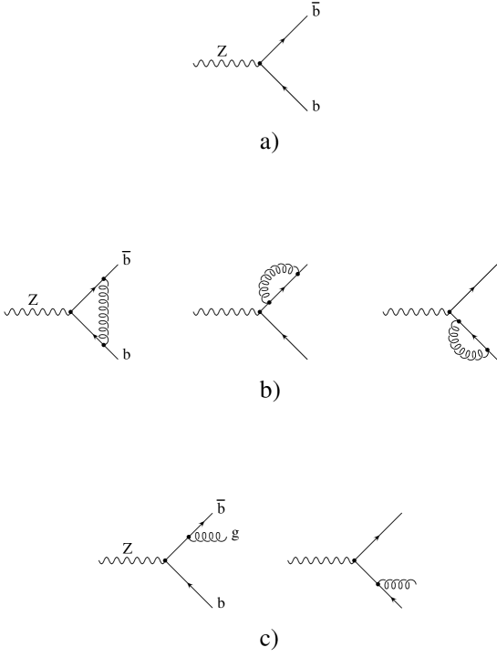
Figure 1. Feynman diagrams contributing to the decay rates $Z\rightarrow b\bar{b}$, $Z\rightarrow b\bar{b}g$ at order $\alpha_{s}$.

At the end, we obtain the well-known result [47]

(2.1) $$\Gamma_{b}=m_{Z}\frac{g^{2}}{c_{W}^{2}64\pi}\left[g_{V}^{2}\left(1+\frac{\alpha_{s}}{\pi}(1+12r_{b})\right)\right.\\ \left.+g_{A}^{2}\left(1-6r_{b}+\frac{\alpha_{s}}{\pi}\left(1-6r_{b}(2\log r_{b}+1)\right)\right)\right]~{}.$$

where $r_{b}=m_{b}^{2}/m_{Z}^{2}$ and $g_{V}$ ($g_{A}$) are the vector (axial-vector) neutral current couplings of the quarks in the Standard Model. At tree level and for the $b$-quark we have

(2.2) $$g_{V}=-1+\frac{4}{3}s^{2}_{W}~{},\hskip 28.45274ptg_{A}=1~{}.$$

We denote by $c_{W}$ and $s_{W}$ the cosine and the sine of the weak mixing angle. Here and below we will conventionally use $\alpha_{s}=\alpha_{s}(m_{Z})$ to designate the value of the running strong coupling constant at the $m_{Z}$-scale.

It is interesting to note the presence of the large logarithm, $\log(m_{b}^{2}/m_{Z}^{2})$, proportional to the quark mass in the axial part of the QCD corrected width, eq. (2.1). The mass that appears in all above calculations should be interpreted as the perturbative pole mass of the quark. But in principle the expression (2.1) could also be written in terms of the so-called running quark mass at the $m_{Z}$ scale by using

(2.3) $$m_{b}^{2}=\bar{m}_{b}^{2}(m_{Z})\left[1+2\frac{\alpha_{s}}{\pi}\left(\frac{4}{3}-\log\frac{m_{b}^{2}}{m_{Z}^{2}}\right)\right]~{}.$$

Then, we see that all large logarithms are absorbed in the running of the quark mass from the $m_{b}$ scale to the $m_{Z}$ scale [38] and we have

(2.4) $$\Gamma_{b}=m_{Z}\frac{g^{2}}{c_{W}^{2}64\pi}\left[g_{V}^{2}\left(1+\frac{\alpha_{s}}{\pi}(1+12\bar{r}_{b})\right)\right.\\ \left.+g_{A}^{2}\left(1-6\bar{r}_{b}+\frac{\alpha_{s}}{\pi}(1-22\bar{r}_{b})\right)\right]~{},$$

where $\bar{r}_{b}=\bar{m}_{b}^{2}(m_{Z})/m_{Z}^{2}$.

This result means that the bulk of the QCD corrections depending on the mass could be accounted for by using tree-level expressions for the decay width but interpreting the quark mass as the running mass. The same point has been stressed in [106] for the hadronic width of the charged Higgs boson. On the other hand, since $\bar{m}_{b}(m_{Z})\approx 3$ GeV is much smaller than the pole mass, $m_{b}\approx 5$ GeV, it is clear that the quark mass corrections are much smaller than expected from the naïve use of the tree-level result with $m_{b}\approx 5$ GeV, which would give mass corrections at the 1.8% level while in fact, once QCD corrections are taken into account, the mass corrections are only at the 0.7% level.

In fact, this remarkable nice feature of the running mass holds to all orders in perturbation theory [37, 39], i.e., all the potentially dangerous terms of the type $m^{2}\log m^{2}/s$ can be absorbed in the $\overline{MS}$ scheme.

2. Jet clustering algorithms

According to our current understanding of the strong interactions, coloured partons, produced in hard processes, are hadronized and, at experiment, one only observes colourless particles. It is known empirically that, in high energy collision, final particles group in several clusters by forming energetic jets, which are related to the primordial partons. Thus, in order to compare theoretical predictions with experiments, it is necessary to define precisely what is a jet in both, parton level calculations and experimental measurements.

At order $\alpha_{s}$, the decay widths of $Z$ into both two and three partons are IR divergent. The two-parton decay rate is divergent due to the massless gluons running in the loops. The $Z$-boson decay width into three-partons has an IR divergence because massless gluons could be radiated with zero energy. The sum, however, is IR finite. Then it is clear that at the parton-level one can define an IR finite two-jet decay rate, by summing the two-parton decay rate and the IR divergent part of the three-parton decay width, e.g. integrated over the part of the phase space which contains soft gluon emission [125]. The integral over the rest of the phase space will give the three-jet decay rate. Thus we need to introduce a “resolution parameter” in the theoretical calculations in order to define IR-safe observables. Obviously, the resolution parameter, which defines the two- and the three-jet parts of the three-parton phase space should be related to the one used in the process of building jets from real particles.

Table 1. The jet-clustering algorithms

Algorithm	Resolution	Combination
EM	$2(p_{i}\cdot p_{j})/s$	$p_{k}=p_{i}+p_{j}$
JADE	$2(E_{i}E_{j})(1-\cos\theta_{ij})/s$	$p_{k}=p_{i}+p_{j}$
E	$(p_{i}+p_{j})^{2}/s$	$p_{k}=p_{i}+p_{j}$
DURHAM	$2\min(E_{i}^{2},E_{j}^{2})(1-\cos\theta_{ij})/s\ \$	$p_{k}=p_{i}+p_{j}$

In the last years the most popular definitions of jets are based on the so-called jet clustering algorithms. These algorithms can be applied at the parton level in the theoretical calculations and also to the bunch of real particles observed at experiment. It has been shown that, for some of the algorithms, the passage from partons to hadrons (hadronization) does not change much the behaviour of the observables [23], thus allowing to compare theoretical predictions with experimental results. In what follows we will use the word particles for both partons and real particles.

In the jet-clustering algorithms jets are defined as follows: starting from a bunch of particles with momenta $p_{i}$ one computes, for example, a quantity like

$$y_{ij}=2\frac{E_{i}E_{j}}{s}(1-\cos\theta_{ij})$$

for all pairs $(i,~{}j)$ of particles. Then one takes the minimum of all $y_{ij}$ and if it satisfies that it is smaller than a given quantity $y_{c}$ (the resolution parameter, y-cut) the two particles which define this $y_{ij}$ are regarded as belonging to the same jet, therefore, they are recombined into a new pseudoparticle by defining the four-momentum of the pseudoparticle according to some rule, for example

$$p_{k}=p_{i}+p_{j}~{}.$$

After this first step one has a bunch of pseudoparticles and the algorithm can be applied again and again until all the pseudoparticles satisfy $y_{ij}>y_{c}$. The number of pseudoparticles found in the end is the number of jets in the event.

Of course, with such a jet definition the number of jets found in an event and its whole topology will depend on the value of $y_{c}$. For a given event, larger values of $y_{c}$ will result in a smaller number of jets. In theoretical calculations one can define cross sections or decay widths into jets as a function of $y_{c}$, which are computed at the parton level, by following exactly the same algorithm. This procedure leads automatically to IR finite quantities because one excludes the regions of phase space that cause trouble. The success of the jet-clustering algorithms is due, mainly, to the fact that the cross sections obtained after the hadronization process agree quite well with the cross-sections calculated at the parton level when the same clustering algorithm is used in both theoretical predictions and experimental analyses.

Figure 2. The phase space for $Z\rightarrow b(p_{1})\bar{b}(p_{2})g(p_{3})$ in the plane $y_{1}=2(p_{1}\cdot p_{3})/s$ and $y_{2}=2(p_{1}\cdot p_{3})/s$ with cuts ($y_{c}=0.04$ and $y_{c}=0.14$) for the different algorithms. The mass of the quark has been set to 10 GeV to enhance mass effects in the plot.

There are different successful jet-clustering algorithms and we refer to [23, 91] for a detailed discussion and comparison of these algorithms in the case of massless quarks.

In the following we will use the four jet-clustering algorithms listed in the table 1, where $\sqrt{s}$ is the total centre of mass energy. In addition to the well-known JADE, E and DURHAM algorithms we will use a slight modification of the JADE scheme particularly useful for analytical calculations with massive quarks [25]. It is defined by the two following equations

$$y_{ij}=\frac{2(p_{i}\cdot p_{j})}{s}$$

and

$$p_{k}=p_{i}+p_{j}.$$

We will denote this algorithm as the EM scheme. For massless particles and at the lowest order E, JADE and EM give the same answers. However already at order $\alpha_{s}^{2}$ they give different answers since after the first recombination the pseudoparticles are not massless anymore and the resolution functions are different.

For massive quarks the three algorithms, E, JADE and EM are already different at order $\alpha_{s}$. The DURHAM ($K_{T}$) algorithm, which has been recently considered in order to avoid exponentiation problems present in the JADE algorithm [33, 31, 23], is of course completely different from the other algorithms we use, both in the massive and the massless cases.

In figure 2 we plotted the phase-space for two values of $y_{c}$ ($y_{c}=0.04$ and $y_{c}=0.14$) for all four schemes (the solid line defines the whole phase space for $Z\rightarrow q\bar{q}g$ with $m_{q}=10$ GeV).

There is an ongoing discussion on which is the best algorithm for jet clustering in the case of massless quarks. The main criteria followed to choose them are based in two requirements:

1. Minimize higher order corrections.

2. Keep the equivalence between parton and hadronized cross sections.

To our knowledge no complete comparative study of the jet-clustering algorithms has been done for the case of massive quarks. The properties of the different algorithms with respect to the above criteria can be quite different in the case of massive quarks from those in the massless case. The first one because the leading terms containing double-logarithms of y-cut ($\log^{2}(y_{c})$) that appear in the massless calculation (at order $\alpha_{s}$) and somehow determine the size of higher order corrections are softened in the case of massive quarks by single-logarithms of $y_{c}$ times a logarithm of the quark mass. The second one because hadronization corrections for massive quarks could be different from the ones for massless quarks.

Therefore, we will not stick to any particular algorithm but rather present results and compare them for all the four algorithms listed in the table 1.

3. Two- and three-jet event rates

At the parton level the two-jet region in the decay $Z\rightarrow b(p_{1})\bar{b}(p_{2})g(p_{3})$ is given, in terms of the variables  $y_{13}$, $y_{23}$ and $y_{12}$, by the following conditions:

(2.5) $$y_{13}<y_{c}\quad\mbox{\rm or}\quad y_{23}<y_{c}\quad\mbox{\rm or}\quad y_{12}<y_{c}~{}.$$

This region contains the IR singularity, $y_{13}=y_{23}=0$ and the rate obtained by the integration of the amplitude over this part of the phase space should be added to the one-loop corrected decay width for $Z\rightarrow b\bar{b}$. The sum of these two quantities is of course IR finite and it is the so-called two-jet decay width at order $\alpha_{s}$. The integration over the rest of the phase space defines the three-jet decay width at the leading order. It is obvious that the sum of the two-jet and three-jet decay widths is independent of the resolution parameter $y_{c}$, IR finite and given by the quantity $\Gamma_{b}=\Gamma(Z\rightarrow b\bar{b}+b\bar{b}g+\cdots)$ calculated in section 1. Therefore we have

(2.6) $$\Gamma_{b}=\Gamma^{b}_{2j}(y_{c})+\Gamma^{b}_{3j}(y_{c})+\cdots~{}.$$

Clearly, at order $\alpha_{s}$, knowing $\Gamma_{b}$ and $\Gamma^{b}_{3j}(y_{c})$ we can obtain $\Gamma^{b}_{2j}(y_{c})$ as well.

The calculation of $\Gamma^{b}_{3j}(y_{c})$ at order $\alpha_{s}$ is a tree-level calculation and does not have any IR problem since the soft gluon region has been excluded from phase space. Therefore the calculation can be done in four dimensions without trouble. The final result can be written in the following form

(2.7) $$\Gamma^{b}_{3j}=m_{Z}\frac{g^{2}}{c_{W}^{2}64\pi}\frac{\alpha_{s}}{\pi}\left(g_{V}^{2}H^{(0)}_{V}(y_{c},r_{b})+g_{A}^{2}H^{(0)}_{A}(y_{c},r_{b})\right)~{},$$

where the superscript ⁽⁰⁾ in the functions $H^{(0)}_{V(A)}(y_{c},r_{b})$ reminds us that this is only the lowest order result. Obviously, the general form 2.7 is independent of what particular jet-clustering algorithm has been used.

In the limit of zero masses, $r_{b}=0$, chirality is conserved and the two functions $H^{(0)}_{V}(y_{c},r_{b})$ and $H^{(0)}_{A}(y_{c},r_{b})$ become identical

(2.8) $$H^{(0)}_{V}(y_{c},0)=H^{(0)}_{A}(y_{c},0)\equiv A^{(0)}(y_{c})~{}.$$

In this case we obtain the known result for the JADE-type algorithms, which is expressed in terms of the function $A^{(0)}(y_{c})$ given by .

(2.9) $$\begin{split}A^{(0)}(y_{c})&=\frac{C_{F}}{2}\left[-\frac{\pi^{2}}{3}+\frac{5}{2}-6y_{c}-\frac{9}{2}y_{c}^{2}+(3-6y_{c})\log\left(\frac{y_{c}}{1-2y_{c}}\right)\right.\\ &+\left.2\log^{2}\left(\frac{y_{c}}{1-y_{c}}\right)+4\mbox{\rm Li}_{2}\left(\frac{y_{c}}{1-y_{c}}\right)\right]~{}.\end{split}$$

The $A^{(0)}(y_{c})$ function is also known analytically for the DURHAM algorithm [33, 31]. Analytical expressions for the functions $H^{(0)}_{V}(y_{c},r_{b})$ and $H^{(0)}_{A}(y_{c},r_{b})$ are given for the EM algorithm in [25].

To see more clearly the size of mass effects we are going to study the following ratio of jet fractions

(2.10) $$R^{bd}_{3}\equiv\frac{\Gamma^{b}_{3j}(y_{c})/\Gamma^{b}}{\Gamma^{d}_{3j}(y_{c})/\Gamma^{d}}=\left(c_{V}\frac{H^{(0)}_{V}(y_{c},r_{b})}{A^{(0)}(y_{c})}+c_{A}\frac{H^{(0)}_{A}(y_{c},r_{b})}{A^{(0)}(y_{c})}\right)\left(1+6r_{b}c_{A}+O(r_{b}^{2})\right)~{},$$

where we have defined

$$c_{V}=\frac{g_{V}^{2}}{g_{V}^{2}+g_{A}^{2}}~{},\quad c_{A}=\frac{g_{A}^{2}}{g_{V}^{2}+g_{A}^{2}}~{}.$$

In eq. (2.10) we have kept only the lowest order terms in $\alpha_{s}$ and $r_{b}$. The last factor is due to the normalization to total rates. This normalization is important from the experimental point of view but also from the theoretical point of view because in these quantities large weak corrections dependent on the top quark mass [8, 18, 19, 16] cancel. Note that, for massless quarks, the ratio $\Gamma^{d}_{3j}(y_{c})/\Gamma^{d}$ is independent on the neutral current couplings of the quarks and, therefore, it is the same for up- and down-quarks and given by the function $A^{(0)}$. This means that we could equally use the normalization to any other light quark or to the sum of all of them (including also the c-quark if its mass can be neglected).

Figure 3. The ratios $R^{bd}_{3}$ (see eq. (2.10)) for the four algorithms. Solid lines correspond to $m_{b}=5$ GeV, dashed lines correspond to $m_{b}=3$ GeV and dotted lines give our estimate of higher order corrections to the $m_{b}=5$ GeV curve. For the JADE algorithm we have also included the results of the analysis of the data collected during 1990-1991 by the DELPHI group [4].

3.1. Estimate of higher order contributions

All previous results come from a tree-level calculation, however, as commented in the introduction, we do not know what is the value of the mass we should use in the final results since the difference among the pole mass, the running mass at $\mu=m_{b}$ or the running mass at $\mu=m_{Z}$ are next-order effects in $\alpha_{s}$.

In the case of the inclusive decay rate we have shown that one could account (with very good precision) for higher order corrections by using the running mass at the $m_{Z}$ scale in the lowest order calculations. Numerically the effect of running the quark mass from $m_{b}$ to $m_{Z}$ is very important.

One could also follow a similar approach in the case of jet rates and try to account for the next-order corrections by using the running quark mass at different scales. We will see below that the dependence of $R^{bd}_{3}$ on the quark mass is quite strong (for all clustering schemes); using the different masses (e.g. $m_{b}$ or $\bar{m}_{b}(M_{Z})$) could amount to almost a factor 2 in the mass effect. This suggests that higher order corrections could be important. Here, however, the situation is quite different, since in the decay rates to jets we have an additional scale given by $y_{c}$, $E_{c}\equiv m_{Z}\sqrt{y_{c}}$, e.g. for $y_{c}=0.01$ we have $E_{c}=9$ GeV and for $y_{c}=0.05$, $E_{c}=20$ GeV. Perhaps one can absorb large logarithms, $\log(m_{b}/m_{Z})$ by using the running coupling and the running mass at the $\mu=m_{Z}$ scale, but there will remain logarithms of the resolution parameter, $\log(y_{c})$. For not very small $y_{c}$ one can expect that the tree-level results obtained by using the running mass at the $m_{Z}$ scale are a good approximation, however, as we already said, the situation cannot be settled completely until a next-to-leading calculation including mass effects is available.

Another way to estimate higher order effects in $R^{bd}_{3}$ is to use the known results for the massless case [55, 84, 86, 122, 23, 91, 57, 87]. Including higher order corrections the general form of eq. (2.7) is still valid with the change $H_{V(A)}^{(0)}(y_{c},r_{b})\rightarrow H_{V(A)}(y_{c},r_{b})$. Now we can expand the functions $H_{V(A)}(y_{c},r_{b})$ in $\alpha_{s}$ and factorize the leading dependence on the quark mass as follows

(2.11) $$H_{V(A)}(y_{c},r_{b})=A^{(0)}(y_{c})+\frac{\alpha_{s}}{\pi}A^{(1)}(y_{c})\\ +r_{b}\left(B_{V(A)}^{(0)}(y_{c},r_{b})+\frac{\alpha_{s}}{\pi}B_{V(A)}^{(1)}(y_{c},r_{b})\right)+\cdots~{}.$$

In this equation we already took into account that for massless quarks vector and axial contributions are identical

Then, we can rewrite the ratio $R^{bd}_{3}$, at order $\alpha_{s}$, as follows

$$R^{bd}_{3}=\left[1+r_{b}\left\{c_{V}\frac{B_{V}^{(0)}(y_{c},r_{b})}{A^{(0)}(y_{c})}\left[1+\frac{\alpha_{s}}{\pi}\left(\frac{B_{V}^{(1)}(y_{c},r_{b})}{B_{V}^{(0)}(y_{c},r_{b})}-\frac{A^{(1)}(y_{c})}{A^{(0)}(y_{c})}\right)\right]\right.\right.$$

$$\left.\left.+c_{A}\frac{B_{A}^{(0)}(y_{c},r_{b})}{A^{(0)}(y_{c})}\left[1+\frac{\alpha_{s}}{\pi}\left(\frac{B_{A}^{(1)}(y_{c},r_{b})}{B_{A}^{(0)}(y_{c},r_{b})}-\frac{A^{(1)}(y_{c})}{A^{(0)}(y_{c})}\right)\right]\right\}\right]$$

(2.12) $$\times\left[1+6\>r_{b}\left\{c_{A}(1+2\frac{\alpha_{s}}{\pi}\log r_{b})-c_{V}2\frac{\alpha_{s}}{\pi}\right\}\right]~{}.$$

The functions $B_{V}^{(0)}(y_{c},r_{b})$ and $B_{A}^{(0)}(y_{c},r_{b})$ where calculated in [25]. The lowest order function for the massless case, $A^{(0)}(y_{c})$, is also known analytically for JADE-type algorithms, eq. (2.9) and refs. [23, 91], and for the DURHAM algorithm [33, 31]. A parametrization of the function $A^{(1)}(y_{c})$ can be found in [23] for the different algorithms . As we already mentioned this function is different for different clustering algorithms. The only unknown functions in eq. (3.1) are $B_{V}^{(1)}(y_{c},r_{b})$ and $B_{A}^{(1)}(y_{c},r_{b})$, which must be obtained from a complete calculation at order $\alpha_{s}^{2}$ including mass effects (at least at leading order in $r_{b}$). The second part of this thesis is devoted to this calculation.

Nevertheless, in order to estimate the impact of higher order corrections in our calculation we will assume for the moment that $B_{V,A}^{(1)}(y_{c},r_{b})/B_{V,A}^{(0)}(y_{c},r_{b})\ll A^{(1)}(y_{c})/A^{(0)}(y_{c})$ and take $A^{(1)}(y_{c})/A^{(0)}(y_{c})$ from [23, 91]. Of course this does not need to be the case but at least it gives an idea of the size of higher order corrections. We will illustrate the numerical effect of these corrections for $R^{bd}_{3}$ in the next subsection. As we will see, the estimated effect of next-order corrections is quite large, therefore in order to obtain the $b$-quark mass from these ratios the calculation of the functions $B_{V,A}^{(1)}(y_{c},r_{b})$ is mandatory.

3.2. Numerical results for $R^{bd}_{3}$ for different clustering algorithms

To complete this section we present the numerical results for $R^{bd}_{3}$ calculated with the different jet-clustering algorithms. For the JADE, E and DURHAM algorithms we obtained the three-jet rate by a numerical integration over the phase-space given by the cuts (see fig. 2). For the EM scheme we used our analytical results [25] which were also employed to cross check the numerical procedure.

In fig. 3 we present the ratio $R^{bd}_{3}$, obtained by using the tree-level expression, eq. (2.10), against $y_{c}$ for $m_{b}=5$ GeV and $m_{b}=3$ GeV. We also plot the results given by eq. (3.1) (with $B_{V,A}^{(1)}(y_{c},r_{b})/B_{V,A}^{(0)}(y_{c},r_{b})=0$) for $m_{b}=5$ GeV, which gives an estimate of higher order corrections. For $y_{c}<0.01$ we do not expect the perturbative calculation to be valid.

As we see from the figure, the behaviour of $R^{bd}_{3}$ is quite different in the different schemes. The mass effect has a negative sign for all schemes except for the E-algorithm. For $y_{c}>0.05$ the mass effects are at the 4% level for $m_{b}=5$ GeV and at the 2% level for $m_{b}=3$ GeV (when the tree level expression is used). Our estimate of higher order effects, with the inclusion of the next-order effects in $\alpha_{s}$ for massless quarks, shifts the curve for $m_{b}=5$ GeV in the direction of the 3 GeV result and amounts to about of 20% to 40% of the difference between the tree-level calculations with the two different masses. For both E and EM schemes we used the higher order results for the E scheme.

Table 2. Results of the three parameter fits of the functions $B_{V,A}^{(0)}(y_{c},r_{b})/A^{(0)}(y_{c})=\sum_{n=0}^{2}k_{V,A}^{(n)}$ log${}^{n}y_{c}$ in the range $0.01<y_{c}<0.20$

Algorithm	$k_{V}^{(0)}\;$	$k_{V}^{(1)}\;$	$k_{V}^{(2)}\;$	$k_{A}^{(0)}\;$	$k_{A}^{(1)}\;$	$k_{A}^{(2)}\;$
EM	$-28.58$	$-14.64$	$-2.72$	$-30.67$	$-13.54$	$-2.61$
JADE	$-13.25$	$-5.19$	$-2.01$	$-15.42$	$-4.13$	$-1.90$
E	$25.97$	$19.04$	$4.68$	$23.39$	$19.81$	$4.71$
DURHAM	$-12.70$	$-4.76$	$-1.69$	$-15.48$	$-4.28$	$-1.65$

Figure 4. The functions $B_{V}^{(0)}/A^{(0)}$ and $B_{A}^{(0)}/A^{(0)}$ for the four algorithms. Dashed lines for $m_{b}=3$ GeV, dotted lines for $m_{b}=5$ GeV and solid lines for our three-parameter fit, eq. (2.13).

To simplify the use of our results we present simple fits in $\log y_{c}$ to the ratios $B_{V,A}^{(0)}(y_{c},r_{b})/A^{(0)}(y_{c})$, which define $R^{bd}_{3}$ at lowest order, for the different clustering algorithms. We use the following parametrization:

(2.13) $$B_{V,A}^{(0)}(y_{c},r_{b})/A^{(0)}(y_{c})=\sum_{n=0}^{2}k_{V,A}^{n}\log^{n}y_{c}~{}.$$

The results of the fits for the range $0.01<y_{c}<0.20$ are presented in table 2.

For completeness we include also in table /reftableA0 a five parameter fit to the LO massless function $A^{(0)}(y_{c})$. For the DURHAM algorithm we take the result from [23]. For the EM, JADE and E algorithms that give the same answer we have fitted the analytical expression of Eq. (2.9).

Table 3. Five parameter fits to the LO massless function $A^{(0)}(y_{c})=\sum_{n=0}^{4}k^{(n)}$ log${}^{n}y_{c}$ in the range $0.01<y_{c}<0.20$

Algorithm	$k^{(0)}\;$	$k^{(1)}\;$	$k^{(2)}\;$	$k^{(3)}\;$	$k^{(4)}\;$
EM/JADE/E	$1.19248$	$2.64729$	$1.359065$	$-.0173022$	$-.001971025$
DURHAM	$.8625$	$1.835$	$1.0745$	$.133$	$.01255$

In fig. 4 we plot the ratios $B_{V,A}^{(0)}(y_{c},r_{b})/A^{(0)}(y_{c})$ as a function of $y_{c}$ for the different algorithms (dashed lines for $m_{b}=5$ GeV, dotted lines for $m_{b}=3$ GeV and solid curves for the result of our fits). As we see from the figure the remnant mass dependence in these ratios (in the range of masses we are interested in and in the range of $y_{c}$ we have considered) is rather small and for actual fits we used the average of the ratios for the two different masses. We see from these figures that such a simple three-parameter fit works reasonably well for all the algorithms.

Concluding this section we would like to make the following remark. In this chapter we discuss the $Z$-boson decay. In LEP experiments one studies the process $e^{+}e^{-}\rightarrow(Z\gamma^{*})\rightarrow b\bar{b}$ and, apart from the resonant $Z$-exchange cross section, there are contributions from the pure $\gamma$-exchange and from the $\gamma-Z$-interference. The non-resonant $\gamma$-exchange contribution at the peak is less than 1% for muon production and in the case of $b$-quark production there is an additional suppression factor $Q_{b}^{2}=1/9$. In the vicinity of the $Z$-peak the interference is also suppressed because it is proportional to $Q_{b}(s-m_{Z}^{2})$ ($\sqrt{s}$ is the $e^{+}e^{-}$ centre of mass energy). We will neglect these terms as they give negligible contributions compared with the uncertainties in higher order QCD corrections to the quantities we are considering.

Obviously, QED initial-state radiation should be taken into account in the real analysis; the cross section for $b$-pair production at the $Z$ resonance can be written as

(2.14) $$\sigma_{b\bar{b}}(s)=\int\sigma^{0}_{b\bar{b}}(s^{\prime})F(s^{\prime}/s)ds^{\prime}$$

where $F(s^{\prime}/s)$ is the well-known QED radiator for the total cross section [17] and, the Born cross section, neglecting pure $\gamma$ exchange contribution and the $\gamma-Z$-interference, has the form

(2.15) $$\sigma^{0}_{b\bar{b}}(s)=\frac{12\pi\Gamma_{e}\Gamma_{b}}{m_{Z}^{2}}\frac{s}{(s-m_{Z}^{2})^{2}+m_{Z}^{2}\Gamma_{Z}^{2}}$$

with obvious notation. Note that $\Gamma_{b}$ in this expression can be an inclusive width as well as some more exclusive quantity, which takes into account some kinematical restrictions on the final state.

4. Discussion and conclusions

In this chapter we have presented a theoretical study of quark-mass effects in the decay of the $Z$-boson into bottom quarks at LO in the strong coupling constant. Furthermore, we have analyzed some three-jet observables which are very sensitive to the value of the quark masses.

For a slight modification of the JADE algorithm (the EM algorithm) we were able to calculate analytically [25] the three-jet decay width of the $Z$-boson into $b$-quarks as a function of the jet resolution parameter, $y_{c}$, and the $b$-quark mass. The answer is rather involved, but can be expressed in terms of elementary functions. Apart from the fact that these analytical calculations are interesting by themselves, they can also be used to test Monte Carlo simulations. For the EM, JADE, E and DURHAM clustering algorithms we have obtained the three-jet decay width by a simple two-dimensional numerical integration. Numerical and analytical results have been compared in the case of the EM scheme.

We discussed quark-mass effects by considering the quantity

$$R^{bd}_{3}=\frac{\Gamma^{b}_{3j}(y_{c})/\Gamma^{b}}{\Gamma^{d}_{3j}(y_{c})/\Gamma^{d}}=1+\frac{m_{b}^{2}}{m_{Z}^{2}}F(m_{b},y_{c})~{}$$

which has many advantages from both the theoretical and the experimental point of views. In particular, at lowest order, the function $F(m_{b},y_{c})$ is almost independent on the quark mass (for the small values of the mass in which we are interested in) and has absolute values ranging from 10 to 35 (depending on $y_{c}$ and on the algorithm), where the larger values are obtained for $y_{c}$ of about $0.01$.

At the lowest order in $\alpha_{s}$ we do not know what is the exact value of the quark mass that should be used in the above equation since the difference between the different definitions of the $b$-quark mass, the pole mass, $m_{b}\approx 5$ GeV, or the running mass at the $m_{Z}$-scale, $\bar{m}_{b}(m_{Z})\approx 3$ GeV, is order $\alpha_{s}$. Therefore, we have presented all results for these two values of the mass and have interpreted the difference as an estimate of higher order corrections. Conversely one can keep the mass fixed and include in $F(m_{b},y_{c})$ higher order corrections already known for the massless case. According to these estimates the $O(\alpha_{s})$ corrections can be about 40% of the tree-level mass effect (depending on the clustering scheme), although we cannot exclude even larger corrections.

By using the lowest order result we find that for moderate values of the resolution parameter, $y_{c}\approx 0.05$, the mass effect in the ratio $R^{bd}_{3}$ is about $4\%$ if the pole mass value of the $b$-quark, $m_{b}\approx 5$ GeV, is used, and the effect decreases to 2% if $m_{b}=3$ GeV. However, in order to extract a meaningful value of the $b$-quark mass from the data it will be necessary to include next-to-leading order (NLO) corrections since the leading mass effect we have calculated does not distinguish among the different definitions of the quark mass (pole mass, running mass at the $m_{b}$ scale or running mass at the $m_{Z}$ scale). Next chapters are devoted to the calculation of the NLO corrections.

Finally, if gluon jets can be identified with enough efficiency [104] another interesting three-jet observable very sensitive to the bottom quark mass is the angular distribution

$$R^{bd}_{\vartheta}\equiv\left.\frac{1}{\Gamma^{b}}\frac{d\Gamma^{b}_{3j}}{d\vartheta}\right/\frac{1}{\Gamma^{d}}\frac{d\Gamma^{d}_{3j}}{d\vartheta},$$

where $\vartheta$ is the minimum of the angles formed between the gluon jet and the quark and antiquark jets. The angular distribution $R^{bd}_{\vartheta}$ was studied at LO in [25]. We will leave its analysis at NLO order for a future work.

Chapter 3 Transition amplitudes at next-to-leading order

In the previous chapter we have seen that some three-jet observables, in particular the following ratio of three-jet decay rate fractions

(3.1) $$R_{3}^{bd}=\frac{\Gamma_{3j}^{b}(y_{c})/\Gamma^{b}}{\Gamma_{3j}^{d}(y_{c})/\Gamma^{d}},$$

are very sensitive to the quark masses and their study at LEP can provide a very interesting experimental information about the bottom quark mass. Among other applications, such study would allow to perform the first measurement of the bottom quark mass far from threshold and, what is more important, it would provide, for the first time, a check of the running of quark masses from scales of the order of $\mu\sim 5(GeV)$ to $\mu=m_{Z}$ in the same way the running of the strong coupling constant has been checked before.

However, as we mentioned, in order to extract a meaningful value of the bottom quark mass from LEP data it is necessary to include next-to-leading order (NLO) strong corrections in $R_{3}^{bd}$ since the LO QCD prediction does not allow to distinguish among the possible theoretical definitions of the quark mass (pole mass, running mass at the $m_{b}$ scale or running mass at the $m_{Z}$ scale) that numerically are quite different.

At the NLO we have contributions from three- and four-parton final states. The three-jet cross section is obtained by integrating both contributions in the three-jet phase space region defined by the jet clustering algorithms considered in the previous chapter: EM, JADE, E and DURHAM. This quantity is infrared finite and well defined, however the three- and four-parton transition amplitudes independently contain infrared singularities. Therefore, some regularization procedure is needed. We use Dimensional Regularization because it preserves the QCD Ward identities. Since at this order we have diagrams with a three gluon vertex it is not possible anymore to regulate the infrared divergences with a gluon mass as it would be possible at the lowest order.

The three-parton transition amplitudes can be expressed in terms of a few scalar one-loop integrals. After UV renormalization we obtain analytical expressions for the terms proportional to the infrared poles and for the finite contributions. The finite contributions are integrated numerically in the three-jet region. The infrared poles will cancel against the four-parton contributions.

The four-parton transition amplitudes are splited into a soft part in the three-jet region and a hard contribution. The soft terms are integrated analytically in arbitrary $D$ dimensions in the region of the phase space containing the infrared singularities. We obtain analytical expressions for the infrared behaviour of the four-parton transition amplitudes and we show how these infrared contributions cancel exactly the infrared singularities of the three-parton transition amplitudes. The hard terms are calculated in $D=4$ dimensions. The remaining phase space integrations giving rise to finite contributions are performed numerically.

In this chapter we consider the NLO corrections to the three-jet decay rate of the $Z$-boson into massive bottom quarks. First we present and classify the matrix elements of the virtual corrections to the process

(3.2) $$Z(q)\rightarrow b(p_{1})+\bar{b}(p_{2})+g(p_{3})~{},$$

and the tree-level processes

(3.3) $$\begin{split}Z(q)&\rightarrow b(p_{1})+\bar{b}(p_{2})+g(p_{3})+g(p_{4})~{},\\ Z(q)&\rightarrow b(p_{1})+\bar{b}(p_{2})+q(p_{3})+\bar{q}(p_{4})~{},\\ Z(q)&\rightarrow b(p_{1})+\bar{b}(p_{2})+b(p_{3})+b(p_{4})~{},\\ \end{split}$$

where $q$ stands for a light quark and the symbols in brackets denote the particle momenta. In the following we will denote by $p_{ij}$ the sum of the momenta of particles labelled $i$ and $j$, $p_{ij}=p_{i}+p_{j}$. In next chapter we calculate the singular IR pieces of these matrix elements in the three-jet region and show how after UV renormalization IR singularities cancel among the one-loop corrected width of $Z\rightarrow b\bar{b}g$ and the tree-level processes (LABEL:todos).

We use Dimensional Regularization to regularize both the UV and the IR divergences [64, 102, 103] with naïve anticommutating $\gamma_{5}$ prescription, see section 6.F of Appendix 6. All the Dirac algebra is performed in $D$-dimensions with the help of the HIP [78] Mathematica 2.0. package. We work in the Feynman gauge.

1. Virtual corrections

The radiative corrections to the process

(3.4) $$Z(q)\rightarrow b(p_{1})+\bar{b}(p_{2})+g(p_{3})~{},$$

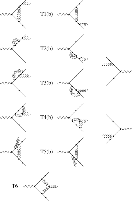
Figure 1. Radiative corrections to the process $Z\rightarrow b\bar{b}g$. Selfenergies in external legs have not been shown. Interference with the lowest order Feynman diagrams, $T0(a)$ and $T0(b)$, gives rise to the $O(\alpha_{s}^{2})$ correction.

are shown in figure 1. They contribute to the three-jet decay rate at $O(\alpha_{s}^{2})$ through their interference with the lowest order Feynman diagrams $T0(a)$ and $T0(b)$. We have not depicted the diagrams with selfenergy insertions in the quark and gluon external legs since their contribution is just the wave function renormalization constant times the square of the lowest order matrix elements.

Only the one loop Feynman diagrams $T1$, $T2$, $T3$ and $T4$ hold UV divergences, the one-loop box integrals of diagrams $T5$ and $T6$ are UV finite since they contain four propagators. Diagrams $T3$ and $T4$ are responsible for the renormalization of the strong coupling constant and diagram $T2$ renormalize the quark mass. The UV divergences of diagram $T1$ are cancelled by the UV piece of the quark wave function renormalization constant. We perform the UV renormalization in a mixed scheme where the strong coupling constant is renormalized in the $\overline{MS}$ scheme while the rest is renormalized in the on-shell scheme. After UV renormalization $T1$, $T2$ and $T3$ become completely finite, $T5$ remains with only simple IR poles whereas $T4$ and $T6$ contain up to double IR divergences. Colour can be used to preliminary classify the one-loop diagrams. The interference of diagrams $T1$ and $T2$ with the lowest order diagrams $T0$ carries a colour factor $C_{F}^{2}$, where $C_{F}=4/3$. Diagrams $T3$ and $T5$ generate a $C_{F}(C_{F}-N_{C}/2)$ colour factor, with $N_{C}=3$ the number of colours, whereas $T4$ and $T6$ produce $C_{F}N_{C}$.

We found the most efficient way to calculate the loop diagrams is to directly perform all the traces over the Dirac matrices on the interference matrix elements to reduce them to a Lorentz scalar, before integrating over the virtual gluon loop momentum $k$. After this, we end up with a series of loop integrals with scalar products of the internal momentum $k$ and the external momenta in the numerator. All these vector and tensor loop integrals can be reduced to simple scalar one loop integrals by following the Passarino-Veltman reduction procedure, see section 6.E of Appendix 6. At the end, our problem is simplified to the calculation of only five one loop three propagator integrals, two infrared divergent scalar box integrals and some well known scalar one- and two-point functions, see Appendix 6. Moreover, the infrared divergent piece of the two four-point functions can be written in terms of two of the three-point one-loop integrals.

2. Emission of two real gluons

The calculation of the transition probability for the process

(3.5) $$Z(q)\rightarrow b(p_{1})+\bar{b}(p_{2})+g(p_{3})+g(p_{4}),$$

from the eight diagrams shown in figure 2 contains in principle 36 terms. However, many of them are related by interchange of momentum labels and, at the end, only 13 transition probabilities need to be calculated. We follow the notation of [55]. The interference of graph $B_{i}$ with $B_{j}$ is written as $B_{ij}$. The relevant 13 transitions probabilities, which we display in fig 3, can be classified into three different subsets depending on the colour factor. In table 1 we give the momentum label interchanges necessary to generate all the transitions probabilities from the thirteen which we choose to calculate.

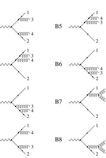
Figure 2. Feynman diagrams contributing to the process $Z\rightarrow b\bar{b}gg$.

Table 1. The interchange table relating the graphs for $Z\rightarrow b\bar{b}gg$.

label	Class A	Class B	Class C
permutation	$C_{F}^{2}$	$C_{F}(C_{F}-\frac{1}{2}N_{C})$	$C_{F}N_{C}$
	B11 B21 B22 B32	B41 B42 B62 B52	B71 B72 B82 B77 B87
$(1\leftrightarrow 2)$	B44 B64 B66 B65	B41 B61 B62 B63	B84 B86 B76 B88 B87
$(3\leftrightarrow 4)$	B44 B54 B55 B65	B41 B51 B53 B52	B74 B75 B85 B77 B87
$(1\leftrightarrow 2)$ $(3\leftrightarrow 4)$	B11 B31 B33 B32	B41 B43 B53 B63	B81 B83 B73 B88 B87

Therefore, it is sufficient to consider the following combinations of transitions amplitudes

(3.6) $$\begin{split}\mbox{\rm Class A}&=\frac{1}{2}B11+2B21+B22+B32,\\ \mbox{\rm Class B}&=\frac{1}{2}B41+2B42+B62+B52,\\ \mbox{\rm Class C}&=2(B71+B72+B82)+\frac{1}{2}(B77+B87),\end{split}$$

plus the interchanges $(1\leftrightarrow 2)$, $(3\leftrightarrow 4)$ and $(1\leftrightarrow 2)$ $(3\leftrightarrow 4)$.

Since only gluons attached to external legs can generate IR divergences in the three-jet region we can see immediately that $B32$ and $B52$ are fully finite, $B21$, $B22$, $B42$ and $B62$ are IR only in gluon labelled as 3 while $B11$ and $B41$ are IR in both gluons, 3 and 4. All the matrix elements of Class A and B are free of quark-gluon collinear divergences since we are working with massive quarks. Therefore, we will find there just IR simple poles, $1/\epsilon$, because only soft singularities remain. On the other hand, we expect IR double poles for diagrams of Class C because the gluon-gluon collinear divergences are still preserved at the three gluon vertex. This argument is not completely true for the transition probabilities $B77$ and $B87$. Both diagrams individually contain IR double poles but when we take into account all the momenta interchanges, i.e., in the square of the sum of diagrams $B7$ and $B8$, double poles cancel. As we will see, these diagrams are related, by Cutkowsky rules, to the diagram with a selfenergy insertion in an external gluon leg. That is the reason why only simple IR poles can appear.

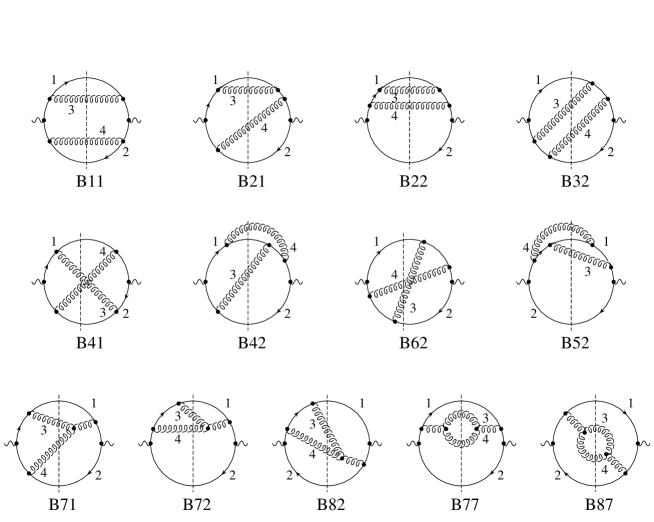
Figure 3. Transitions probabilities for the process $Z\rightarrow b\bar{b}gg$ On-shell particles are indicated by the dashed line and the numbers refer to the momentum labels. All the other transition probabilities can be obtained by permutation of momentum labels.

We must sum only over the two physical polarizations of the produced gluons. This is most easily accomplished by summing over the polarizations with

(3.7) $$\sum_{pol}\varepsilon^{\mu*}\varepsilon^{\nu}=-g^{\mu\nu}~{},$$

but including $B7$- and $B8$-like Feynman diagrams with “external” ghosts to take into account of the fact that the gluon current is not conserved.

3. Emission of four quarks

Lastly, we calculate the matrix elements for the decay width of the $Z$-boson into four quarks. Two processes have to be considered

(3.8) $$\begin{split}Z(q)&\rightarrow b(p_{1})+\bar{b}(p_{2})+q(p_{3})+\bar{q}(p_{4}),\\ Z(q)&\rightarrow b(p_{1})+\bar{b}(p_{2})+b(p_{3})+\bar{b}(p_{4}),\end{split}$$

where $q$ stands for a light quark.

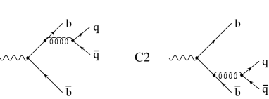
Figure 4. Feynman diagrams contributing to the process $Z\rightarrow b\bar{b}q\bar{q}$ where $q$ stands for a light quark.

For the first process we restrict to the case where the pair of bottom-antibottom quarks is emitted from the primary vertex, figure 4. Similar Feynman diagrams, where the heavy quark pair is radiated off a light $q\bar{q}$ system, are also possible. Despite the fact that $b$ quarks are present in this four fermion final state, the natural prescription is to assign these events to the light channels. Obviously, they must be subtracted experimentally. This should be possible since their signature is characterized by a large invariant mass of the light quark pair and a small invariant mass of the bottom system. Since four fermion final states, $b\bar{b}q\bar{q}$, originate from the interference between $q\bar{q}$ and $b\bar{b}$ induced amplitudes to assign them to a partial decay rate of a particular flavour is evidently not possible in a straightforward manner.

The massless calculation [55, 91, 23] to which we want to compare our results was performed by summing over all the allowed flavours. No ambiguity appears in this case. The massless QCD prediction is proportional to the the sum over all the squared vector and axial-vector couplings

(3.9) $$\sum_{N_{F}}(g_{Vi}^{2}+g_{Ai}^{2}),$$

although this factor cancels in the three-jet decay rate ratios. Our choice is the appropriate to get 1 for the massive over the massless three-jet fraction ratio in the limit of massless bottom quarks. Conclusively, there is no way to solve this ambiguity and hence in the case of four fermion final states the theoretical analysis should be tailored to the specific experimental cuts.

The transition probabilities $C11$, $C22$ and $C12$ can generate infrared divergences, soft and quark-quark collinear singularities, in the three-jet region due to the light quarks. In principle these divergences can manifest as double poles.  Nevertheless, as in the case of the gluon-gluon collinear divergences of the transition probabilities $B77$, $B88$ and $B87$ double poles cancel in the sum because these transition amplitudes are related, by Cutkowsky rules, to the diagrams with a gluon selfenergy insertion in the Born amplitudes $T0(a)$ and $T0(b)$, where only simple infrared poles can appear. All the other transition probabilities we will treat in this section are infrared finite.

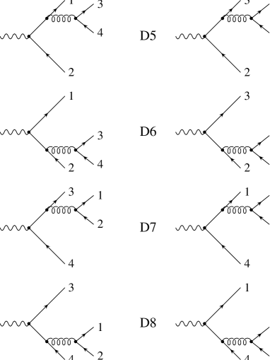
Figure 5. Feynman diagrams contributing to the decay width of the $Z$-boson into four massive bottom quarks.

We consider now the emission of four bottom quarks. As in the case of the emission of two real gluons, from the eight diagrams shown in figure 5 we should compute only twelve transition probabilities because many of the, in principle, possible 36 terms are related by interchange of momentum labels.

Table 2. The interchange table relating the graphs for $Z\rightarrow b\bar{b}b\bar{b}$.

label	Class D	Class E	Class F
permutation	$C_{F}T_{R}$	$C_{F}(C_{F}-\frac{1}{2}N_{C})$	$C_{F}$
	D11 D12 D22	D18 D25 D15 D28 D17 D26	D13 D23 D24
$(1\leftrightarrow 3)$	D55 D56 D66	D45 D16 D15 D46 D35 D62	D57 D67 D68
$(2\leftrightarrow 4)$	D77 D78 D88	D27 D38 D37 D28 D17 D48	D57 D58 D68
$(1\leftrightarrow 3)$ $(2\leftrightarrow 4)$	D33 D34 D44	D36 D47 D37 D46 D35 D48	D13 D14 D24

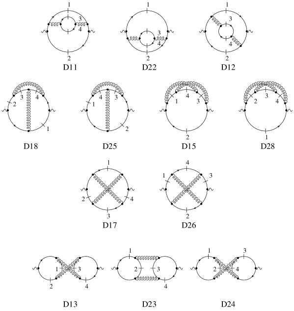
Figure 6. Transition probabilities for the process $Z\rightarrow b\bar{b}b\bar{b}$. On-shell particles are indicated by a short cutting line and the numbers refer to the momentum labels. All the other transition probabilities can be obtained by exchange of momentum labels.

It is sufficient to consider the following combinations of transitions amplitudes

(3.10) $$\begin{split}\mbox{\rm Class D}&=D11+2D12+D22~{},\\ \mbox{\rm Class E}&=-(D15+D28+D17+D26+2(D18+D25))~{},\\ \mbox{\rm Class F}&=D13+2D23+D24~{},\end{split}$$

plus the interchanges $(1\leftrightarrow 3)$, $(2\leftrightarrow 4)$ and $(1\leftrightarrow 3)$ $(2\leftrightarrow 4)$. Due to Fermi statistics there is a relative minus sign for diagrams $D5$ to $D8$ that is reflected in the transition probabilities of Class E and ensures that each helicity amplitude vanish when both fermions (antifermions) have identical quantum numbers. Furthermore, we will call

(3.11) $$\mbox{\rm Class G}=\mid C1+C2\mid^{2}$$

that evidently carries the same colour factor as the Class D transition probabilities, $C_{F}T_{R}$, where $T_{R}=1/2$.

The transition amplitudes of Class F are called in the literature [39], singlet contributions because they contain two different fermion loops and hence can be splited into two parts by cutting gluon lines only. The first contribution to the vectorial part arises at $O(\alpha_{s}^{3})$ as a consequence of the non-abelian generalization of Furry’s theorem. Singlet contributions to the axial part appear already at $O(\alpha_{s}^{2})$.

Lastly, let’s comment on the Class F-like case where a bottom quark is running in one of the loops and a light quarks is in the other. This would produce a term proportional to the product of the vector-axial couplings of both quarks, $g_{Ab}g_{Aq}$, and represents the interference of diagrams of figure 4 with those we have not considered. Nevertheless, since the vector-axial coupling of up and down quarks are different in sign, $g_{Au}=-g_{Ad}=1$, their contribution will cancel when summing over all the light quarks and only the diagram with bottom quarks running on both loops will survive.

This section concludes our classification of the transition probabilities we must compute in order to achieve the NLO QCD prediction for the three-jet decay rate of the $Z$-boson into massive quarks. As we have commented, IR divergences are the main problem that appears when we try to compute them. In the next chapter we will show how to extract from these transition amplitudes the divergent pieces and how to keep away the finite parts. We will integrate analytically the divergent contributions over phase space and we will show how infrared divergences are cancelled.

Chapter 4 Infrared cancellations

In the previous chapter we have presented the NLO virtual and real corrections to the decay width of the $Z$-boson into three jets. We were able to reduce the contribution of the real corrections to the calculation of a few transition probabilities and the contribution of the virtual corrections to the calculation of a few scalar one-loop n-point functions, see Appendix 7. After UV renormalization of the loop diagrams we still encounter a plethora of IR divergences which should cancel with the soft and collinear singularities of the tree level diagrams when we integrate over the three-jet region of phase space. The theorems of Bloch-Nordsiek [26] and Kinoshita-Lee-Nauenberg [82, 97] guaranty such cancellation.

We have classified our transition probabilities following their colour factors. It is clear that the cancellation of IR divergences can only occur inside groups of diagrams with the same colour factor. The problem of the IR cancellation can be simplified if we find a criteria to split our transition probabilities into different groups such that the cancellation of IR singularities can be shown independently. The key is to depict them as bubble diagrams as we did in figure 3 and figure 6 and perform all the possible cuts that could lead to three-jet final states, see figure 1.

It is not difficult to convince ourselves that transition probabilities of Class A can be related only to the insertion of the quark selfenergy in the external legs of the lowest order diagram $T0$. The transition probabilities of Class B have the same IR structure as the one loop diagram $T5$. Besides, $B71$, $B72$ and $B82$ lie in the same group as the one loop diagrams $T4$ and $T6$. And finally, $B77$, $B87$, $C11$, $C12$, $D11$ and $D22$ are related with the gluon selfenergy insertion diagram at $T0$.

In the following sections we are going to show analytically how the cancellation of the IR divergences occurs following the previous classification.

1. Soft divergences

The phase space of $n+1$ particles can be written as the product of the $n$-body phase space times the integral over the energy and solid angle of the extra particle [132]. In arbitrary $D=4-2\epsilon$ dimensions we have

(4.1) $$dPS(n+1)=\frac{1}{2(2\pi)^{D-1}}E^{D-3}\>dE\>d\Omega\>dPS(n)~{}.$$

Suppose $E_{3}$ is the energy of one soft gluon: $E_{3}<w$ where $w$, with $w$ very small, is an upper cut on the soft gluon energy. Let’s consider

(4.2) $$\int_{0}^{w}E_{3}^{D-3}dE_{3}\>d\Omega\frac{1}{(2p_{1}\cdot p_{3})^{2}}~{},$$

that appears for instance in the four parton transition amplitudes of Class A, where $p_{3}$ is the momentum of the gluon and $p_{1}$ is the momentum of the quark. After integration over the trivial angles we find

(4.3) $$\frac{2\pi^{\frac{D}{2}-1}}{4\Gamma\left(\frac{D}{2}-1\right)}\int_{0}^{w}dE_{3}E_{3}^{D-5}\int_{-1}^{1}dx\frac{(1-x^{2})^{\frac{D-4}{2}}}{(E_{1}-\mbox{\rm\bf p}_{1}x)^{2}}~{},$$

with $\mbox{\rm\bf p}_{1}$ the modulus of the threemomentum. In the eikonal region we can suppose $E_{1}$ almost independent from $E_{3}$

(4.4) $$E_{1}\simeq\frac{\sqrt{s}}{2}(1-y_{24})~{},$$

with $y_{24}=2(p_{2}\cdot p_{4})/m_{Z}^{2}$. The integral over $E_{3}$ can be easily done and gives a simple infrared pole in $\epsilon$. Since the $x$ dependent part is completely finite we can expand in $\epsilon$ before the integral over this variable is performed. The final result we get is as follows

(4.5) $$\frac{1}{2(2\pi)^{D-1}}\int_{0}^{w}E_{3}^{D-3}dE_{3}d\Omega\frac{1}{(2p_{1}\cdot p_{3})^{2}}=\\ \frac{1}{16\pi^{2}}\frac{(4\pi)^{\epsilon}}{\Gamma(1-\epsilon)}\frac{w^{D-4}}{D-4}\frac{1}{E_{1}^{2}-\mbox{\rm\bf p}_{1}^{2}}\left[1-\epsilon\left(\frac{E_{1}}{\mbox{\rm\bf p}_{1}}\log\frac{E_{1}-\mbox{\rm\bf p}_{1}}{E_{1}+\mbox{\rm\bf p}_{1}}+2\log 2\right)\right]~{}.$$

Let’s consider now

(4.6) $$\int_{0}^{w}E_{3}^{D-3}dE_{3}d\Omega\frac{1}{(2p_{1}\cdot p_{3})(2p_{2}\cdot p_{3})}~{},$$

that appears in the four parton transition amplitudes of Class B, with $p_{2}$ the momentum of the antiquark. In this case we can perform a Feynman parametrization over the two momenta scalar products

(4.7) $$\frac{1}{(p_{1}\cdot p_{3})(p_{2}\cdot p_{3})}=\int_{0}^{1}dy\frac{1}{[p_{3}\cdot(p_{1}+(p_{2}-p_{1})y)]^{2}}~{}.$$

We get therefore the same integral structure as in Eq. (4.5), integral over $y$ left, but with the fourmomentum

(4.8) $$p_{A}=p_{1}+(p_{2}-p_{1})y~{}.$$

instead of $p_{1}$. For the divergent part we get

(4.9) $$\frac{1}{2(2\pi)^{D-1}}\int_{0}^{w}E_{3}^{D-3}dE_{3}d\Omega\frac{1}{(2p_{1}\cdot p_{3})(2p_{2}\cdot p_{3})}=\\ -\frac{1}{16\pi^{2}}\frac{(4\pi)^{\epsilon}}{\Gamma(1-\epsilon)}\frac{w^{D-4}}{D-4}\left[\frac{2}{(y_{12}+2r_{b})\beta_{12}}\log c_{12}+O(\epsilon)\right]~{},$$

where

(4.10) $$r_{b}=m_{b}^{2}/m_{Z}^{2}~{},\qquad\beta_{12}=\sqrt{1-\frac{4r_{b}}{y_{12}+2r_{b}}}~{},\qquad c_{12}=\frac{1-\beta_{12}}{1+\beta_{12}}~{}.$$

It is not easy to get a full analytical expression for the finite part. Nevertheless, the integral over the $y$ parameter can be done numerically, using for instance a simple GAUSS integration. Notice this last integral has the same divergent structure as the scalar one loop $C05$ function defined in Eq. (6.17).

The matrix element of diagram $B2$ reads

(4.11) $$B2=i\frac{g}{4c_{W}}g_{s}^{2}(T^{a}T^{b})\bar{u}(p_{1})\\ \left\{\gamma_{\nu}\frac{1}{\not p\hskip 3.01385pt_{13}-m_{b}}\gamma_{\sigma}\frac{1}{\not p\hskip 3.01385pt_{134}-m_{b}}\gamma_{\mu}(g_{V}+g_{A}\gamma_{5})\right\}v(p_{2})\varepsilon_{a}^{*\nu}(p_{3})\varepsilon_{b}^{*\sigma}(p_{4})\varepsilon_{Z}^{\mu}(q)~{},$$

where $T^{a}=\lambda^{a}/2$ are the colour Gell-Mann matrices, $\varepsilon_{a}^{*\nu}$, $\varepsilon_{b}^{*\sigma}$ and $\varepsilon_{Z}^{\mu}$ stand for the polarization vector of the two gluons and the $Z$-boson and $g_{V}$ ($g_{A}$) are the vector (axial-vector) neutral current couplings of the quarks in the Standard Model. At tree-level and for the bottom quark we have

(4.12) $$g_{V}=-1+\frac{4}{3}s_{W}^{2},\qquad g_{A}=1~{}.$$

We denote by $c_{W}$ and $s_{W}$ the cosine and the sine of the weak mixing angle.

With the help of the equation of motion we can write

(4.13) $$\bar{u}(p_{1})\gamma^{\nu}(\not p\hskip 3.01385pt_{13}+m_{b})=\bar{u}(p_{1})(\gamma^{\nu}\not p\hskip 3.01385pt_{3}+2p_{1}^{\nu})~{}.$$

In the limit of gluon labelled as 3 soft, $p_{3}\rightarrow 0$, it reduces to $2p_{1}^{\nu}\bar{u}(p_{1})$ and $B2$ behaves as the Born amplitude $T0(a)$

(4.14) $$B2\simeq-g_{s}(T^{a})\frac{2p_{1}^{\nu}}{y_{13}}T0(a)\varepsilon_{a}^{*\nu}(p_{3})~{}.$$

Hence, in this limit we find for the transition amplitude $B22$ the following result

(4.15) $$B22\simeq-g_{s}^{2}C_{F}\frac{4r_{b}}{y_{13}^{2}}\mid T0(a)\mid^{2}~{}.$$

Integrating over phase space with the help of Eq. (4.5) we find

(4.16) $$dPS(4)B22\simeq C_{F}\frac{\alpha_{s}}{4\pi}\frac{(4\pi)^{\epsilon}}{\Gamma(1-\epsilon)}\frac{2w^{-2\epsilon}}{\epsilon}dPS(3)[1+O(\epsilon)]\mid T0(a)\mid^{2}~{}.$$

Same argument can be applied to the transitions amplitudes $B11$ and $B21$ for which we get

(4.17) $$\begin{split}B11&\sim\frac{1}{\epsilon}(\mid T0(a)\mid^{2}+\mid T0(b)\mid^{2})~{},\\ B21&\sim\frac{1}{\epsilon}T0(a)^{*}T0(b)~{}.\end{split}$$

For the moment we don’t need to consider $B32$ because it is infrared finite. Since the transition amplitude $B11$ can be soft in both gluons, labelled 3 and 4, we have splited off the contribution of each one by performing a partial fractioning

(4.18) $$\frac{1}{y_{13}^{3}y_{24}^{2}}=\frac{1}{y_{13}^{2}+y_{24}^{2}}\left(\frac{1}{y_{13}^{2}}+\frac{1}{y_{24}^{2}}\right)~{}.$$

The first term should be integrated in the 1-3 system, second term in the equivalent 2-4 system. Relabelling in both cases the remaining hard gluon as 3 we arrive at the result quoted in Eq. (4.17).

Finally, taking into account all the momenta permutations, we find for the eikonal contribution of the diagrams of Class A to the decay width of the Z-boson into massive bottom quarks the following result

(4.19) $$\Gamma_{w}(\mbox{\rm Class A})=\frac{8}{2!}C_{F}\frac{\alpha_{s}}{4\pi}\frac{(4\pi)^{\epsilon}}{\Gamma(1-\epsilon)}\frac{w^{-2\epsilon}}{\epsilon}\frac{1}{2m_{Z}}\int dPS(3)\mid T0(a)+T0(b)\mid^{2}~{},$$

where $2!$ is the statistical factor and

(4.20) $$\begin{split}&\frac{16c_{W}^{2}}{g^{2}}\frac{1}{g_{s}^{2}C_{F}}\mid T0(a)+T0(b)\mid^{2}=\\ &g_{V}^{2}\left[8(D-2+4r_{b})\frac{h_{p}}{y_{13}^{2}y_{23}^{2}}+2(D-2)^{2}\left(\frac{y_{13}}{y_{23}}+\frac{y_{23}}{y_{13}}\right)+4(D-2)(D-4)\right]\\ +&g_{A}^{2}(D-2)\left[8(1-4r_{b})\frac{h_{p}}{y_{13}^{2}y_{23}^{2}}+2(D-2+4r_{b})\left(\frac{y_{13}}{y_{23}}+\frac{y_{23}}{y_{13}}\right)+4(D-4+4r_{b})\right]~{},\end{split}$$

with

(4.21) $$h_{p}=y_{13}y_{23}(1-y_{13}-y_{23})-r_{b}(y_{13}+y_{23})^{2}~{},$$

is the squared lowest order transition amplitude in $D$-dimensions.

The wave function renormalization constant of the quark propagator contains two pieces

(4.22) $$\begin{split}Z_{2}=1-&C_{F}\frac{\alpha_{s}}{4\pi}\tau_{0}\left[\Delta_{UV}-\log\frac{m_{b}^{2}}{\mu^{2}}+2\right]\\ -&C_{F}\frac{\alpha_{s}}{4\pi}\left\{(3-\tau_{0})\left[\Delta_{IR}-\log\frac{m_{b}^{2}}{\mu^{2}}\right]+2(2-\tau_{0})\right\}~{},\end{split}$$

where $\Delta=1/\epsilon-\gamma_{E}+\log 4\pi$ and $\tau_{0}$ is the gauge parameter, $\tau_{0}=1$ since we work in the Feynman gauge. The first one is the usual UV piece and cancels the UV divergences of diagram $T1$. The second piece comes from the residue of the $\overline{MS}$ renormalized propagator in the pole. When we include it in the self-energy diagrams of external quarks we get a contribution

(4.23) $$-2\frac{\alpha_{s}}{4\pi}C_{F}2\Delta_{IR}\frac{1}{2m_{Z}}\int dPS(3)\mid T0(a)+T0(b)\mid^{2}~{},$$

which exactly cancels the IR divergences of (4.19).

As we made with $B2$ in (4.14) the matrix element of diagram $B4$ reads

(4.24) $$B4\simeq g_{s}(T^{a})\left(C_{F}-\frac{N_{C}}{2}\right)\frac{2p_{2}^{\nu}}{y_{23}}T0(a)\varepsilon_{a}^{*\nu}(p_{3})~{},$$

for gluon labelled as 3 soft. The colour factor comes from the following properties of the $SU(3)$ Gell-Mann matrices

(4.25) $$\begin{split}&[T_{a},T_{b}]=i\>f_{abc}T^{c}~{},\\ &f_{abc}T^{b}T^{c}=i\frac{N_{C}}{2}T_{a}~{}.\end{split}$$

Therefore, the transition amplitude $B42$ behaves as

(4.26) $$B42\simeq g_{s}^{2}\left(C_{F}-\frac{N_{C}}{2}\right)\frac{4(p_{1}\cdot p_{2})}{y_{13}y_{23}}\mid T0(a)\mid^{2}~{},$$

in the eikonal region. Including phase space, from Eq. (4.9) we get for its divergent piece

(4.27) $$dPS(4)B42\simeq\left(C_{F}-\frac{N_{C}}{2}\right)\frac{\alpha_{s}}{4\pi}\frac{(4\pi)^{\epsilon}}{\Gamma(1-\epsilon)}\\ \frac{2w^{-2\epsilon}}{\epsilon}dPS(3)\left[\frac{y_{12}}{(y_{12}+2r_{b})\beta_{12}}\log c_{12}+O(\epsilon)\right]\mid T0(a)\mid^{2}~{}.$$

As before we find for the other transition amplitudes of Class B the following behaviour

(4.28) $$\begin{split}B41&\sim\frac{1}{\epsilon}[T0(a)^{*}T0(b)+T0(b)^{*}T0(a)]~{},\\ B62&\sim\frac{1}{\epsilon}T0(a)^{*}T0(b)~{},\end{split}$$

where for $B41$ we made the following partial fractioning

(4.29) $$\frac{1}{y_{13}y_{23}y_{14}y_{24}}=\frac{1}{y_{13}y_{23}+y_{14}y_{24}}\left(\frac{1}{y_{13}y_{23}}+\frac{1}{y_{14}y_{24}}\right)~{}.$$

The final answer for this class of diagrams reads

(4.30) $$\Gamma_{w}(\mbox{\rm Class B})=\frac{8}{2!}\left(C_{F}-\frac{N_{C}}{2}\right)\frac{\alpha_{s}}{4\pi}\frac{(4\pi)^{\epsilon}}{\Gamma(1-\epsilon)}\\ \frac{w^{-2\epsilon}}{\epsilon}\frac{1}{2m_{Z}}\int dPS(3)\frac{y_{12}}{(y_{12}+2r_{b})\beta_{12}}\log c_{12}\mid T0(a)+T0(b)\mid^{2}~{}.$$

Let’s consider now the one-loop box diagram $T5$

(4.31) $$\begin{split}T5(a)&=-g_{s}^{3}\bar{u}(p_{1})(T^{b}T^{a}T^{b})\int\frac{d^{D}k}{(2\pi)^{D}}\\ &\frac{\gamma^{\sigma}[(\not k\hskip 3.01385pt+\not p\hskip 3.01385pt_{1})+m_{b}]\gamma^{\nu}[(\not k\hskip 3.01385pt+\not p\hskip 3.01385pt_{13})+m_{b}]\gamma^{\mu}(g_{V}+g_{A}\gamma_{5})[(\not k\hskip 3.01385pt-\not p\hskip 3.01385pt_{2})+m_{b}]\gamma^{\sigma^{\prime}}}{k^{2}[(k+p_{1})^{2}-m_{b}^{2}][(k+p_{13})^{2}-m_{b}^{2}][(k-p_{2})^{2}-m_{b}^{2}]}\\ &\left[g_{\sigma\sigma^{\prime}}-(1-\tau_{0})\frac{k_{\sigma}k_{\sigma^{\prime}}}{k^{2}}\right]v(p_{2})\varepsilon_{a}^{*\nu}(p_{3})\varepsilon_{Z}^{\mu}(q)~{}.\end{split}$$

Again we apply the equation of motion of the quarks

(4.32) $$\begin{split}\bar{u}(p_{1})\gamma^{\sigma}[(\not k\hskip 3.01385pt+\not p\hskip 3.01385pt_{1})+m_{b}]&=\bar{u}(p_{1})(\gamma^{\sigma}\not k\hskip 3.01385pt+2p_{1}^{\sigma})~{},\\ [(\not k\hskip 3.01385pt-\not p\hskip 3.01385pt_{2})+m_{b}]\gamma^{\sigma^{\prime}}v(p_{2})&=(\not k\hskip 3.01385pt\gamma^{\sigma^{\prime}}-2p_{2}^{\sigma^{\prime}})v(p_{2})~{},\end{split}$$

at both sides of the previous equation. Dropping all the $\not k\hskip 3.01385pt$ factors in the numerator and expanding the third propagator for small loop momentum we arrive to

(4.33) $$T5(a)\simeq-\frac{\alpha_{s}}{4\pi}(4p_{1}\cdot p_{2})C05(y_{12})T0(a)~{},$$

where $C05$ is defined in Eq. (6.14). It is straitforward to see from the solution (6.17) to the one-loop integral $C05$ how the interference of the one loop amplitude of Eq. (4.33) with the lowest order amplitude $T0$ cancels exactly the IR divergences of the diagrams grouped in Class B, Eq. (4.30).

2. Collinear divergences

To show how the cancellation of the infrared divergences for diagrams of Class C occurs is quite more difficult. Since we have gluon-gluon collinear divergences it is not enough to make a cut in the energy of one of the gluons, as we made in the previous section, to extract the divergent piece. In this case the appropriate variable over which we have to impose a cut is $y_{34}=2(p_{3}\cdot p_{4})/m_{Z}^{2}$ as it includes both kind of divergences, soft and collinear, in the limit of $y_{34}\rightarrow 0$. Looking at the four partons phase space in the so-called “system 3-4” defined in section 7.B of appendix 7 we can notice several things. First, in the limit $y_{34}\rightarrow 0$ the function $h_{p}$ that defines the limits of the phase space reduces to the three parton phase space $h_{p}$ function (7.4). Second, the momentum $p_{34}=p_{3}+p_{4}$ behaves as the momentum of a pseudo on-shell gluon because $p_{34}^{2}\rightarrow 0$ in this limit. Therefore, it is possible to factorize from the four-body phase space a three-body phase space with an effective gluon of momentum $p_{34}$. Only integration over the extra variables should be performed to show the cancellation of the infrared divergences.

2.1. Diagrams containing gluon-gluon collinear divergences

Let’s consider the following phase space integral

(4.34) $$PS(4)\frac{1}{y_{13}y_{34}}~{},$$

in the called system 3-4 (7.15), where as usual $p_{1}$ denotes the momentum of the quark and $p_{3}$ and $p_{4}$ are the two gluon momenta. This integral can be soft for gluon labelled as 3 and collinear because of the scalar product of the two gluon momenta $y_{34}$. In the eikonal region, $y_{34}<w$ with $w$ very small, we can decompose the four body-phase space as the product of a three-body phase space in terms of variables $y_{134}$ and $y_{234}$ times the integral over $y_{34}$ and the two angular variables $v$ and $\theta^{\prime}$

(4.35) $$PS(4)\frac{1}{y_{13}y_{34}}=PS(3)(y_{134},y_{234})\\ \frac{S}{16\pi^{2}}\frac{(4\pi)^{\epsilon}}{\Gamma(1-\epsilon)}\int_{0}^{w}dy_{34}\int_{0}^{1}dv(v(1-v))^{-\epsilon}\frac{1}{N_{\theta^{\prime}}}\int_{0}^{\pi}d\theta^{\prime}\sin^{-2\epsilon}\theta^{\prime}\frac{y_{34}^{-1-\epsilon}}{y_{13}}~{}.$$

$S=1/2!$, the statistical factor. In the 3-4 system the two-momenta invariant $y_{13}$ can be written in terms of the integration variables as

(4.36) $$y_{13}=\frac{1}{2}\left(y_{134}-\sqrt{y_{134}-4r_{b}y_{34}}(1-2v)\right)~{}.$$

The $y_{13}$ factor is independent of the $\theta^{\prime}$ angle so we can get rid of this first integral. Second observation, $y_{13}$ contain a piece independent of the $v$ angle and another one that is odd under the interchange $v\leftrightarrow(1-v)$. With the help of this symmetry

(4.37) $$\frac{1}{2}\left(\frac{1}{A+f(v)}+\frac{1}{A-f(v)}\right)=\frac{A}{A^{2}-f(v)^{2}}~{},$$

we can avoid the use of the square root of Eq. (4.36) and write our integral as

(4.38) $$PS(4)\frac{1}{y_{13}y_{34}}=PS(3)(y_{134},y_{234})\frac{S}{16\pi^{2}}\frac{(4\pi)^{\epsilon}}{\Gamma(1-\epsilon)}$$

$$\int_{0}^{w}y_{34}^{-1-\epsilon}dy_{34}\int_{0}^{1}dv(v(1-v))^{-\epsilon}\frac{2y_{134}}{y_{134}^{2}-(y_{134}^{2}-4r_{b}y_{34})(1-2v)^{2}}~{}.$$

After integration over $y_{34}$ we get the first infrared pole

(4.39) $$\frac{-1}{\epsilon}\frac{w^{-\epsilon}}{2y_{134}}\int_{0}^{1}dv(v(1-v))^{-1-\epsilon}{}_{2}F_{1}[1,-\epsilon,1-\epsilon,-\frac{r_{b}w(1-2v)^{2}}{y_{134}v(1-v)}]~{}.$$

Some simple mathematical manipulations [85, 3, 115, 113] allow us to express the hypergeometric function in terms of a simple dilogarithm

(4.40) $$\begin{split}{}_{2}F_{1}[1,-\epsilon,1-\epsilon,-\frac{a}{b}]&=\left(\frac{b}{a+b}\right)^{-\epsilon}{}_{2}F_{1}[-\epsilon,-\epsilon,1-\epsilon,\frac{a}{a+b}]\\ &=\left(\frac{b}{a+b}\right)^{-\epsilon}\left[1+\epsilon^{2}Li_{2}\left(\frac{a}{a+b}\right)+O(\epsilon^{3})\right]~{},\end{split}$$

to finally obtain

(4.41) $$\frac{-1}{\epsilon}\frac{w^{-\epsilon}}{2y_{124}}\int_{0}^{1}dv(v(1-v))^{-1-2\epsilon}\left(v(1-v)+A(1-2v)^{2}\right)^{\epsilon}\\ \left[1+\epsilon^{2}Li_{2}\left(\frac{A(1-2v)^{2}}{v(1-v)+A(1-2v)^{2}}\right)+O(\epsilon^{3})\right]~{},$$

with $A=r_{b}w/y_{134}^{2}$. The contribution of the dilogarithm function reduces to its value at the border of the integration region, i.e., just additional $Li_{2}(1)=\pi^{2}/6$ factors to the finite part. Further contributions would be next order in $\epsilon$. Therefore, it is enough to analyze the first two factors. This integrand is symmetric under the interchange $v\leftrightarrow(1-v)$. We perform the integral only in half of the integration region and apply the following change of variables

(4.42) $$u=4v(1-v)~{},$$

to get

(4.43) $$\frac{-1}{\epsilon}\frac{w^{-\epsilon}A^{\epsilon}}{y_{134}}2^{4\epsilon}\int_{0}^{1}duu^{-1-2\epsilon}(1-u)^{-1/2}\left[1-\left(1-\frac{1}{4A}\right)u\right]^{\epsilon}~{},$$

which gives again an hypergeometric function

(4.44) $$\frac{-1}{\epsilon}\frac{1}{y_{134}}\left(\frac{r_{b}}{y_{134}^{2}}\right)^{\epsilon}2^{4\epsilon}\sqrt{\pi}\frac{\Gamma(-2\epsilon)}{\Gamma(\frac{\displaystyle 1}{\displaystyle 2}-2\epsilon)}{}_{2}F_{1}[-\epsilon,-2\epsilon,\frac{1}{2}-2\epsilon,1-\frac{1}{4A}]~{}.$$

The hypergeometric function is already $1+O(\epsilon^{2})$ but now it is not possible to write it in terms of a simple dilogarithm function. If we are interested just in the pole structure we can stop here. Observe that neither the double pole or the simple one depend on the eikonal cut $w$. To get the complete finite part further mathematical manipulations must be performed on the hypergeometric function.

Be

$${}_{2}F_{1}[-\epsilon,-2\epsilon,\frac{1}{2}-2\epsilon,1-\frac{1}{4A}]=$$

(4.45) $$(4A)^{2\epsilon}\Gamma(\frac{\displaystyle 1}{\displaystyle 2}-2\epsilon)\left\{\frac{\Gamma(\epsilon)}{\Gamma(-\epsilon)\Gamma(\frac{\displaystyle 1}{\displaystyle 2})}{}_{2}F_{1}[-2\epsilon,\frac{1}{2}-\epsilon,1-\epsilon,4A]\right.\\ +\left.\frac{\Gamma(-\epsilon)}{\Gamma(-2\epsilon)\Gamma(\frac{\displaystyle 1}{\displaystyle 2}-\epsilon)}{}_{2}F_{1}[-\epsilon,\frac{1}{2},1+\epsilon,4A]\right\}~{}.$$

For $w$ enough small, $w\ll y_{134}^{2}/r_{b}$, we can use the Gauss series [3] to expand the hypergeometric functions around $A\rightarrow 0$. The final result we obtain is as follows

(4.46) $$\begin{split}dPS(4)\frac{1}{y_{13}y_{34}}=dPS(3)(y_{134},y_{234})&\\ \frac{S}{16\pi^{2}}\frac{(4\pi)^{\epsilon}}{\Gamma(1-\epsilon)}\frac{1}{y_{134}}\left\{\frac{1}{2\epsilon^{2}}+\frac{1}{2\epsilon}\log\frac{r_{b}}{y_{134}^{2}}\right.+&\frac{1}{4}\log^{2}\frac{r_{b}}{y_{134}^{2}}-\frac{1}{2}\log^{2}A-\frac{\pi^{2}}{4}\\ -&2A\log A-A^{2}(2+3\log A)+O(A^{3})\biggr{\}}~{}.\end{split}$$

Notice we get the same infrared poles as in the one-loop three point function $C03$, Eq. (6.16), appearing in the one-loop amplitudes $T4$ and $T6$.

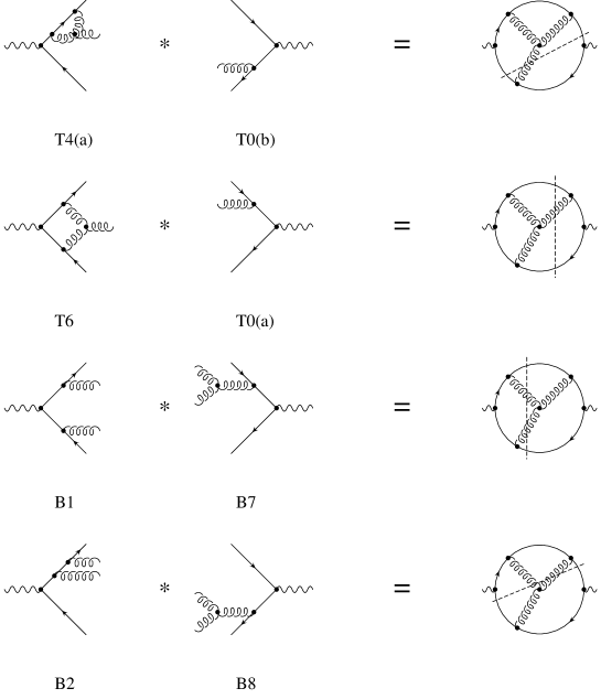
Figure 1. Cuts over a bubble diagram with three gluon vertex and transition probabilities with related IR structures in the three-jet region. The other possible cuts lead to two-jet final states.

2.2. Gluon selfenergy-like diagrams

We discuss now the infrared behaviour of the transition amplitudes $B77$, $B87$, $C11$, $C12$ and those grouped in Class D. Diagrams of Class D, that correspond to the emission of four bottom quarks, are infrared finite since the infrared singularities are softened into logarithms of the bottom quark mass and can be calculated in $D=4$ dimensions and integrated numerically without any trouble.

The infrared divergences of the transition probabilities $C11$ and $C12$ that correspond to the emission of a pair of light quarks can be regulated by introducing a small light quark mass. Nevertheless, we chose Dimensional Regularization. Since kinematically massless quarks and gluons are equivalent we can integrate the $B77$, $B87$, $C11$ and $C12$ transition probabilities in the same system 3-4.

For the transition amplitudes $B77$ and $B87$ we have to solve the following basic phase space integral

(4.47) $$PS(4)\frac{1}{y_{34}}~{}.$$

As we said we work in the system 3-4, (7.15). All the integrals factorize giving rise to a simple result in the eikonal region

(4.48) $$dPS(4)\frac{1}{y_{34}}=\frac{S}{16\pi^{2}}\frac{(4\pi)^{\epsilon}}{\Gamma(1-\epsilon)}\left[-\frac{1}{\epsilon}+\log w-2\right]dPS(3)(y_{134},y_{234})~{}.$$

As we have mentioned, the transition probabilities $B77$ and $B87$ contain in principle double infrared poles. Nevertheless, the sum of them, i.e., the square of the sum of amplitudes $B7$ and $B8$, is proportional to

(4.49) $$\left(\frac{y_{13}}{y_{134}}-\frac{y_{23}}{y_{234}}\right)^{2}\frac{1}{y_{34}^{2}}~{}.$$

Expanding for small values of $y_{34}$ we find

(4.50) $$4v(1-v)\cos^{2}\theta^{\prime}\left(\frac{1-2r_{b}-y_{134}-y_{234}}{y_{134}y_{234}}-\frac{r_{b}}{y_{134}^{2}}-\frac{r_{b}}{y_{234}^{2}}\right)\frac{1}{y_{34}}+O(y_{34}^{-1/2})~{}.$$

Therefore, only simple poles can appear. Same arguments apply for the transition probabilities $C11$ and $C12$, that we grouped under Class G.

This completes the calculation for the collinear divergent diagrams grouped in Class C and Class G. Intermediate steeps are rather involved but the final result can be written in a simple manner in terms of the Born amplitude

(4.51) $$\begin{split}\Gamma_{w}(\mbox{\rm Class C})&=\frac{1}{2!}N_{C}\frac{\alpha_{s}}{4\pi}\frac{(4\pi)^{\epsilon}}{\Gamma(1-\epsilon)}\frac{1}{2m_{Z}}\int dPS(3)(y_{13},y_{23})\\ \Bigg{\{}&4\left[\frac{w^{-\epsilon}}{\epsilon}+2+I^{w}(y_{23})+I^{w}(y_{13})\right]\\ +&\left[\frac{10}{3}\frac{w^{-\epsilon}}{\epsilon}+\frac{62}{9}\right]\Bigg{\}}\mid T0(a)+T0(b)\mid^{2}~{},\end{split}$$

where

(4.52) $$I^{w}(x)=\frac{1}{2\epsilon^{2}}+\frac{1}{2\epsilon}\log\frac{r_{b}}{x^{2}}+\frac{1}{4}\log^{2}\frac{r_{b}}{x^{2}}-\frac{1}{2}\log^{2}\frac{r_{b}w}{x^{2}}-\frac{\pi^{2}}{4}+O\left(\frac{r_{b}w}{x^{2}}\right)~{},$$

and

(4.53) $$\begin{split}\Gamma_{w}(\mbox{\rm Class G})&=T_{R}(N_{F}-1)\frac{\alpha_{s}}{4\pi}\frac{(4\pi)^{\epsilon}}{\Gamma(1-\epsilon)}\frac{1}{2m_{Z}}\int dPS(3)(y_{13},y_{23})\\ &\left[-\frac{4}{3}\frac{w^{-\epsilon}}{\epsilon}-\frac{20}{9}\right]\mid T0(a)+T0(b)\mid^{2}~{},\end{split}$$

with $T_{R}=1/2$ and $(N_{F}-1)$ the number of light quarks.

Since, as we mentioned, $p_{34}$ behaves in the IR region as the momentum of a pseudo on-shell massless particle, $p_{34}^{2}\rightarrow 0$, we have relabelled the integration variables $(y_{134},y_{234})$ as $(y_{13},y_{23})$. First contribution of Eq. (4.51) comes from the transition probabilities $B71$, $B72$ and $B82$ and cancels the IR divergences of the one-loop diagrams $T4$ and $T6$. To show it explicitly needs a considerable amount of algebra. We get terms proportional to the simple infrared pole and terms proportional to the $C03$ one-loop function that exactly cancels the $I^{w}$ function divergent piece. Nevertheless, we can justify such cancellation using simple graphical arguments as we have shown in figure 1. In fact, this was the main argument we used to classify all the transition probabilities in different groups such that IR divergences cancel independently. Second contribution comes from the transition amplitudes $B77$ and $B87$ and together with the Class G contribution is cancelled against

(4.54) $$-2\frac{\alpha_{s}}{4\pi}\left[\frac{5}{6}N_{C}-\frac{2}{3}T_{R}(N_{F}-1)\right]\Delta_{IR}\frac{1}{2m_{Z}}\int dPS(3)\mid T0(a)+T0(b)\mid^{2}~{},$$

with $\Delta_{IR}=1/\epsilon-\gamma_{E}+\log 4\pi$, coming from the gluon wave function renormalization constant.

Chapter 5 Numerical results and conclusions

We have seen in the previous chapter how infrared singularities cancel between the three parton one-loop and the four parton tree-level diagrams contributing at NLO to the $Z$-boson three-jet decay rate. In fact, due to the Bloch-Nordsiek [27] and Kinoshita-Lee-Nauenberg [83, 96] theorems, we knew from the beginning they should do. The cancellation of the IR divergences is of course the first test of our calculation. Nevertheless, the real challenge is in the calculation of the finite contributions.

Ultraviolet singularities arise in loop integrals once the integration over the internal momentum is performed and in the form of a singular Gamma function. Moreover, we are allowed to expand in $\epsilon$ before integrating over the Feynman parameters. Main problem of IR divergences is that they appear always at the borders. At the border of the one unit side box defined by the Feynman parameters in loop integrals, and at the border of the phase space for the tree-level transition amplitudes. Therefore, we are forced to perform in arbitrary $D$-dimensions the full calculation in the infrared region. This makes the computation of their finite contributions extremely difficult. Even for the finite contributions strong cancellations occur among different groups of diagrams making very difficult the numerical approach.

We have taken as guide line the massless result [23, 91, 55] although the IR structure in the massive case is completely different from the massless one. With massive quarks we loose all the quark-gluon collinear divergences. The amplitudes behave better in the IR region. The disadvantage however is the mass itself because we have to perform quite more complicated loop and phase space integrals. Furthermore, the gluon-gluon collinear divergences, leading to IR double poles and whose finite contributions are harder to solve, are still present.

Our procedure was as follows. For the one-loop transition probabilities we were able to reduce the loop integrals to a few scalar one-loop n-point functions whose finite parts are under control, see Appendix 6. We drop all the terms proportional to $1/\epsilon^{2}$ and $1/\epsilon$ since, as we have seen in chapter 4, they cancel against the four parton real corrections to the three-jet decay rate. Since the boundary of the three-body phase space, including cuts, is a complicated function we perform the remaining phase space integration over the one-loop finite contributions with the help of VEGAS [99, 100], an adaptative Monte Carlo FORTRAN algorithm for multidimensional integration.

We have seen that the four parton transition amplitudes have a simple and well known behaviour in the soft and collinear regions, basically proportional to the lowest order three parton transition probabilities, making the integration over these regions of the four-body phase space feasible analytically. Our strategy was to exclude from the numerical integration domain the singular regions. We impose a cut, we called $w$, with $w$ very small, in the energy of the soft gluons. For the diagrams with collinear singularities we cut on the two momenta invariant variable $y_{34}=2(p_{3}\cdot p_{4})/s$. In the excluded phase space regions we replace the transitions amplitudes by their limiting values and perform analytically the integration over this phase space singular region in arbitrary $D=4-2\epsilon$ dimensions (we only need to analytically integrate three of the five independent variables defining the four-body phase space). The analytic integration gives the IR poles in $1/\epsilon^{2}$ and $1/\epsilon$ that again we drop and some finite contributions that we still have to integrate numerically over an effective three-body phase space. Finally, the full transition probabilities, calculated in $D=4$ dimensions, are integrated numerically in the three-jet region of the four-body phase space above the $w$ cut.

Both results, the semi-analytical one and the full-numerical one depend on the cut $w$. First requirement should be of course the sum of them is independent of $w$. We have to keep in mind this is an approximate method since we have substituted in the singular region the transition amplitudes by their limiting values. The smaller value of $w$ the better approximation we get. On the other hand, since the integrand near the boundaries of the singular region increases steeply, typically like $\log w$, the $w$ cut can not be very small otherwise we immediately loose accuracy in the numerical integration. In practice we should find a compromise over these two conflicting requirements to achieve the best efficiency. We have studied the $w$-dependence of the final result and we found $w/m_{Z}\sim 10^{-5}$ provides a good approximation.

This method is called in the literature [90] the phase space slicing method as we exclude from the numerical integration domain a slice of the phase space. It was applied for instance by [66, 67, 12, 72, 11]. Another method of analytic cancellation of IR singularities, called the subtraction method, has been developed by [55, 91, 56, 58, 92, 101, 34]. The idea is to subtract and add back a quantity that must be a proper approximation to the differential real cross section such that it has the same pointwise singular behaviour (in $D$-dimensions) and is analytically integrable (in $D$-dimensions) over the one parton subspace leading to the soft and collinear divergences.

1. Tests

As we mentioned the introduction of massive quarks complicate extremely the calculation of the three-jet decay rate in spite of the fact that some of the singularities are softened into logarithms of the quark mass. Therefore, to check our results against already tested simpler calculations is a crucial point.

The knowledge of the transition amplitudes is a well established result in the massless case [55, 57, 87] as well as the three- and four-jet fractions in the JADE, E and DURHAM jet clustering algorithms [23, 91]. The four-jet decay rate has been calculated for massive quarks for instance in [13, 14, 69].

First test was to check our four parton final state transition amplitudes in the four-jet region. Since the four-jet phase space region is free of IR singularities in both the massless and the massive case we are allowed to neglect the quark mass. The comparison with the massless result [55, 23, 91] was successful as well as with the massive calculations [13, 14, 69]. Nevertheless, this is not a conclusive proof. First, this checks only the four parton final state transition amplitudes. Second, the calculation can be performed in four dimensions. And finally, since the four-jet region is completely IR finite, it does not matter the way we write the transition amplitudes, the Monte Carlo phase space integration converges quite quickly. The main problem is not how to calculate the transition probabilities but the way we write them. The ERT citeEllis81 transition amplitudes can not be directly used when we try to calculate the three-jet decay rate.

1.1. Massless three-jet decay rate at next-to-leading order

Next steep was to test our procedure of analytic cancellation of IR divergences over the ERT [55] transition amplitudes in the three-jet region and to recalculate the $A^{(1)}(y_{c})$ function that defines the NLO massless correction to the three-jet decay rate. Furthermore, this test allowed us to check our phase space, algorithm cuts and numerical integration routines in the massless limit. We remind the three-jet decay rate can be written as

(5.1) $$\Gamma^{b}_{3j}=m_{Z}\frac{g^{2}}{c_{W}^{2}64\pi}\frac{\alpha_{s}}{\pi}[g_{V}^{2}H_{V}(y_{c},r_{b})+g_{A}^{2}H_{A}(y_{c},r_{b})],$$

Table 1. Results of the five parameter fits to the function $A^{(1)}(y_{c})=\sum_{n=0}^{4}k_{n}$ log${}^{n}y_{c}$ in the range $0.01<y_{c}<0.20$

Algorithm	$k_{0}\qquad$	$k_{1}\qquad$	$k_{2}\qquad$	$k_{3}\qquad$	$k_{4}\qquad$
EM	$17.25(12)$	$20.37(10)$	$-7.320(47)$	$-12.621(21)$	$-1.9200(45)$
JADE	$17.872(26)$	$26.599(21)$	$1.265(10)$	$-9.5644(48)$	$-1.8547(10)$
E	$12.41(13)$	$20.22(10)$	$-1.912(49)$	$-11.173(23)$	$-1.7920(47)$
DURHAM	$-.021(13)$	$-.533(11)$	$-3.8826(55)$	$-3.3720(25)$	$-.46956(49)$

Figure 1. The function $A^{(1)}$ which determines the massless NLO three-jet decay rate for the EM, JADE, E and DURHAM jet clustering algorithms.

where $r_{b}=m_{b}^{2}/m_{Z}^{2}$, $y_{c}$ is the resolution parameter, and $g_{V}$ and $g_{A}$ are the vector and the axial-vector neutral current quark couplings. At tree-level and for the bottom quark $g_{V}=-1+4s_{W}^{2}/3$ and $g_{A}=1$ in the Standard Model. In the massless limit we wrote

(5.2) $$H_{V(A)}=A^{(0)}(y_{c})+\frac{\alpha_{s}}{\pi}A^{(1)}(y_{c}),$$

where we have taken into account that for massless quarks vector and axial contributions are identical

The EM jet clustering algorithm was introduced for the first time in [25] because in this algorithm at LO the two- and three-jet decay rates can be calculated analytically for massive quarks. The function $A^{(1)}(y_{c})$ is therefore unknown in this case. We have calculated it for the first time. Furthermore, we have not only tested but tried to improve the accuracy in the knowledge of the $A^{(1)}(y_{c})$ function for the JADE and DURHAM algorithms. Quark mass corrections are very small in these two jet clustering algorithms, specially in DURHAM, and a better determination of the $A^{(1)}(y_{c})$ function contributes to a better understanding of the quark mass effects.

To simplify the use of our results and to compare them with the [23, 91] result we have performed a simple five parameter $\log y_{c}$ power series fit to the $A^{(1)}(y_{c})$ function for the different jet clustering algorithms

(5.3) $$A^{(1)}(y_{c})=\sum_{n=0}^{4}k_{n}\log^{n}y_{c}~{}.$$

The results of our fits for the range $0.01<y_{c}<0.20$ are presented in table 1. We plot in figure 1 the $A^{(1)}(y_{c})$ function for the four algorithms we have considered.

1.2. The massless limit test

Finally, we integrate in the three-jet region the massive quark transition amplitudes we have calculated and we try to see if extrapolating our result to the massless limit we can reach the $A^{(1)}(y_{c})$ function of the previous section. This is the main test of our calculation.

In figures 2 and 3 we present our result for the vectorial contribution to the $O(\alpha_{s}^{2})$ three-jet decay rate of the Z-boson into bottom quarks for the JADE and E algorithms. We have performed the calculation for different values of the bottom quark mass from $1$ to $5(GeV)$ for fixed $y_{c}$. We remind we factorized the leading dependence on the quark mass in the functions $H_{V(A)}$ as follows

(5.4) $$H_{V(A)}=A^{(0)}(y_{c})+r_{b}B_{V(A)}^{(0)}(y_{c},r_{b})+\frac{\alpha_{s}}{\pi}\left(A^{(1)}(y_{c})+r_{b}B_{V(A)}^{(1)}(y_{c},r_{b})\right).$$

Figure 2. NLO contribution to the three-jet decay rate of $Z\rightarrow b\bar{b}$ for bottom quark masses from $1$ to $5(GeV)$ and fixed $y_{c}$ in the Jade algorithm. Big circle is the massless case.

Figure 3. NLO contribution to the three-jet decay rate of $Z\rightarrow b\bar{b}$ for bottom quark masses from $1$ to $5(GeV)$ and fixed $y_{c}$ in the E algorithm. Big circle is the massless case.

In the JADE algorithm we can see that for big values of $y_{c}$ the NLO corrections due to the quark mass are very small and below the massless result. Notice they increase quite a lot for small values of $y_{c}$ and give a positive correction that will produce a change in the slope of the LO prediction for $R_{3}^{bd}$. In any case we recover the massless limit and a linear parametrization in the quark mass squared would provide a good description. The DURHAM and EM algorithm would exhibit a very similar behaviour to the JADE algorithm.

The E algorithm behaves also linearly in the quark mass squared although only for big values of $y_{c}$. Corrections in the E algorithm are always very strong. The reason is the following, the resolution parameter for the E algorithm explicitly incorporates the quark mass, $y_{ij}=(p_{i}+p_{j})/s$, i.e., for the same value of $y_{c}$ we are closer to the two-jet IR region and the difference from the other algorithms is precisely the quark mass. This phenomenon is already manifested at the LO. For massive quarks the behaviour of the E algorithm is completely different from the other algorithms. It is difficult to believe in the E algorithm as a good prescription for physical applications since mass corrections as so big. However for the same reason, it seems to be the best one for testing massive calculations.

Furthermore, since we have encoded the ERT formulas, we were able to perform some partial tests, not only the final three-jet decay rate. The IR structure of the massless transition amplitudes of [55] is completely different from the massive case. This means, we can not test our calculation amplitude by amplitude. Nevertheless, in the previous chapters we were able to split our transition probabilities into different groups such that IR singularities cancel independently. Checking can be performed group by group. The difference lies in the singularities that are softened into $\log r_{b}$ for massive quarks. They must cancel too. In the massless case we have to cancel these singularities analytically. In the massive case we do it numerically. We have not calculated analytically the terms proportional to $\log r_{b}$. A future improvement of our calculation could be to do that.

2. Massive three-jet decay rate at next-to-leading order

To conclude, we present our final calculation for the $B^{(1)}_{V(A)}(y_{c},r_{b})$ functions defining the NLO mass correction to the three-jet ratio $R_{3}^{bd}$ in the four jet clustering algorithms EM, JADE, E and DURHAM, see figures 4, 5, 6 and 7. We have performed the calculation for $m_{b}=3(GeV)$ and $m_{b}=5(GeV)$ pole masses. Error bars come from the Monte Carlo phase space numerical integration. As before, to simplify the use of our results, we have performed simple five parameter $\log y_{c}$ power series fits to the ratio of the function $B^{(1)}_{V,A}(y_{c},r_{b})$ and the massless NLO function $A^{(1)}(y_{c})$. We use the following parametrization:

(5.5) $$B^{(1)}_{V,A}(y_{c},r_{b})/A^{(1)}(y_{c})=\sum_{n=0}^{4}k^{n}_{V,A}\log^{n}y_{c}~{}.$$

The results of our fits for the range $0.01<y_{c}<0.20$ ($0.025<y_{c}<0.20$ for JADE and E algorithms) are presented in table 2. For the moment we perform independent fits to the $m_{b}=3(GeV)$ and $m_{b}=5(GeV)$ results.

Table 2. Results of the five parameter fits to the function $B^{(1)}_{V,A}(y_{c})/A^{(1)}(y_{c})=\sum_{n=0}^{4}k^{n}_{V,A}$ log${}^{n}y_{c}$ in the range $0.01<y_{c}<0.20$ for EM and DURHAM algorithms and $0.025<y_{c}<0.20$ for JADE and E for bottom quark pole masses of $3(GeV)$ and $5(GeV)$.

Algorithm	$k_{0}\qquad$	$k_{1}\qquad$	$k_{2}\qquad$	$k_{3}\qquad$	$k_{4}\qquad$
EM
$k_{V}(3GeV)$	$6.9(48)$	$90.2(30)$	$84.15(93)$	$27.79(27)$	$2.957(47)$
$k_{A}$	$-54.5(16)$	$-43.32(94)$	$-6.85(28)$	$3.024(84)$	$0.664(14)$
$k_{V}(5GeV)$	$-10.7(52)$	$65.4(31)$	$71.98(93)$	$25.39(27)$	$2.798(47)$
$k_{A}$	$-38.4(16)$	$-24.09(95)$	$1.49(28)$	$4.731(83)$	$0.800(14)$
JADE
$k_{V}(3GeV)$	$396.3(39)$	$676.8(25)$	$410.59(92)$	$109.93(32)$	$10.941(75)$
$k_{A}$	$85.5(12)$	$170.40(75)$	$111.77(28)$	$33.256(97)$	$3.747(23)$
$k_{V}(5GeV)$	$224.2(38)$	$403.2(25)$	$249.43(92)$	$68.35(32)$	$6.989(75)$
$k_{A}$	$94.0(12)$	$181.87(75)$	$117.55(28)$	$34.689(97)$	$3.893(23)$
E
$k_{V}(3GeV)$	$589.6(52)$	$1080.1(32)$	$759.5(12)$	$234.24(40)$	$27.599(92)$
$k_{A}$	$-584.7(17)$	$-1059.1(10)$	$-673.70(38)$	$-183.63(13)$	$-17.305(30)$
$k_{V}(5GeV)$	$621.8(52)$	$1112.7(32)$	$767.8(12)$	$233.85(40)$	$27.343(92)$
$k_{A}$	$-535.4(17)$	$-975.3(10)$	$-622.80(38)$	$-170.11(13)$	$-16.004(30)$
DURHAM
$k_{V}(3GeV)$	$105.0(38)$	$183.4(25)$	$107.27(77)$	$27.17(23)$	$2.498(38)$
$k_{A}$	$69.8(11)$	$110.34(76)$	$61.53(23)$	$15.364(69)$	$1.421(11)$
$k_{V}(5GeV)$	$132.5(38)$	$212.5(25)$	$120.40(77)$	$29.99(23)$	$2.739(38)$
$k_{A}$	$74.9(11)$	$116.88(76)$	$65.51(23)$	$16.435(69)$	$1.525(11)$

DURHAM seems to be the most promising jet algorithm to keep under control the higher order corrections since not only the NLO massless function $A^{(1)}(y_{c})$ is the smallest but also because the ratio $B^{(1)}_{V,A}(y_{c},r_{b})/A^{(1)}(y_{c})$ holding the mass information is the smallest too. We get $B^{(1)}_{V,A}(y_{c},r_{b})/A^{(1)}(y_{c})\simeq-10$. On the other hand, mass corrections are so big in the E algorithm, for the reasons we mentioned in the previous section, and LO and NLO predictions for $R_{3}^{bd}$ are so different that perturbation theory probably breaks down in this case. The normalized mass correction in the JADE and EM algorithms are around two and three times the mass correction in the DURHAM algorithm, we obtain $B^{(1)}_{V,A}(y_{c},r_{b})/A^{(1)}(y_{c})\simeq-20,-30$ respectively, although still under reasonable values.

In all the three algorithms, EM, JADE and DURHAM, the $B^{(1)}_{V,A}(y_{c},r_{b})/A^{(1)}(y_{c})$ ratio is negative since massive quarks are expected to radiate less gluons than massless quarks. Nevertheless, for enough small value of the resolution parameter $y_{c}$, depending on the algorithm, the mass correction becomes positive and steeply increasing. This means there is one point where the NLO mass corrections are zero.

This phenomenon happens because for enough small values of $y_{c}$ the four parton transition probabilities contribute mainly to the four-jet fraction and therefore in the three-jet region the virtual corrections dominate. This translates into a change in the slope of the LO prediction for $R_{3}^{bd}$, i.e., the NLO prediction for $R_{3}^{bd}$ going down for small values of $y_{c}$ becomes increasing and closer to unity. For the range of the resolution parameter $y_{c}$ we are considering, $0.01<y_{c}<0.20$, we can see in figures 4 and 5 this already occurs in the EM and JADE algorithm for $y_{c}\simeq 0.02$. For the DURHAM algorithm we have to wait for a resolution parameter smaller than $y_{c}<0.01$. In fact, although this phenomenon is a sign that perturbation theory breaks down and therefore our perturbative prediction is meaningless, we can see in figure 8 that for the preliminary DELPHI results in the DURHAM algorithm this tendency really happens.

2.1. Estimate of higher order contributions

Up to now we made all the calculations with the assumption $\mu^{2}=s=m^{2}_{Z}$. This does not restrict the validity of our result since the $\mu$ dependence is completely determined by the Renormalization Group. The scale dependence is introduced in $R_{3}^{bd}$ by the replacements

(5.6) $$\begin{split}\alpha_{s}(m_{Z})&\rightarrow\alpha_{s}(\mu),\\ r_{b}&\rightarrow\bar{r}_{b}(\mu)\left\{1+2\frac{\alpha_{s}(\mu)}{\pi}\left[\frac{4}{3}-\log\frac{\bar{m}_{b}^{2}(\mu)}{\mu^{2}}\right]\right\}.\end{split}$$

Assuming we have factorized in the functions $B_{V,A}^{(0)}(y_{c},r_{b})$ and $B_{V,A}^{(1)}(y_{c},r_{b})$ the leading dependence on the quark mass and the remnant mass dependence is soft , i.e., $B_{V,A}^{(i)}(y_{c},r_{b})\simeq B_{V,A}^{(i)}(y_{c})$ the three-jet fraction ratio $R_{3}^{bd}$ reads

(5.7) $$R_{3}^{bd} = \Bigg{[}1+\bar{r}_{b}(\mu)\Bigg{\{}$$

$$c_{V}\frac{B_{V}^{(0)}(y_{c})}{A^{(0)}(y_{c})}\left[1+\frac{\alpha_{s}(\mu)}{\pi}\left(\frac{B_{V}^{(1)}(y_{c})}{B_{V}^{(0)}(y_{c})}+2\left(\frac{4}{3}-\log\frac{\bar{m}^{2}_{b}(\mu)}{\mu^{2}}\right)-\frac{A^{(1)}(y_{c})}{A^{(0)}(y_{c})}\right)\right]$$

$$+ c_{A}\frac{B_{A}^{(0)}(y_{c})}{A^{(0)}(y_{c})}\left[1+\frac{\alpha_{s}(\mu)}{\pi}\left(\frac{B_{A}^{(1)}(y_{c})}{B_{A}^{(0)}(y_{c})}+2\left(\frac{4}{3}-\log\frac{\bar{m}^{2}_{b}(\mu)}{\mu^{2}}\right)-\frac{A^{(1)}(y_{c})}{A^{(0)}(y_{c})}\right)\right]\Bigg{\}}\Bigg{]}$$

$$\times \left[1+6\bar{r}_{b}(\mu)\left\{c_{A}\left(1+2\frac{\alpha_{s}(\mu)}{\pi}\left(\frac{4}{3}-\log\frac{s}{\mu^{2}}\right)\right)-c_{V}2\frac{\alpha_{s}(\mu)}{\pi}\right\}\right]~{}.$$

At the lowest order we define

(5.8) $$\bar{r}_{b}^{0}=\frac{R_{3}^{bd}-1}{c_{V}\frac{\displaystyle B_{V}^{(0)}(y_{c})}{\displaystyle A^{(0)}(y_{c})}+c_{A}\left(\frac{\displaystyle B_{A}^{(0)}(y_{c})}{\displaystyle A^{(0)}(y_{c})}+6\right)}~{},$$

with $\bar{m}_{b}^{0}=m_{Z}\sqrt{\bar{r}_{b}^{0}}$. We can solve iteratively Eq. (5.7) to get

(5.9) $$\begin{split}\bar{r}_{b}(m_{Z})&=\left.\bar{r}_{b}^{0}\left(\frac{\alpha_{s}(m_{Z})}{\alpha_{s}(\mu)}\right)^{\frac{\displaystyle 4\gamma_{0}}{\displaystyle\beta_{0}}}\right/\Bigg{[}1+\frac{\alpha_{s}(\mu)}{\pi}\frac{\bar{r}_{b}^{0}}{R_{3}^{bd}-1}\Bigg{\{}\\ &c_{V}\frac{B_{V}^{(0)}(y_{c})}{A^{(0)}(y_{c})}\left(\frac{B_{V}^{(1)}(y_{c})}{B_{V}^{(0)}(y_{c})}+2\left(\frac{4}{3}-2\log\frac{\bar{m}^{0}_{b}}{\mu}\right)-\frac{A^{(1)}(y_{c})}{A^{(0)}(y_{c})}\right)\\ +&c_{A}\frac{B_{A}^{(0)}(y_{c})}{A^{(0)}(y_{c})}\left(\frac{B_{A}^{(1)}(y_{c})}{B_{A}^{(0)}(y_{c})}+2\left(\frac{4}{3}-2\log\frac{\bar{m}^{0}_{b}}{\mu}\right)-\frac{A^{(1)}(y_{c})}{A^{(0)}(y_{c})}\right)\\ +&12c_{A}\left(\frac{4}{3}-\log\frac{s}{\mu^{2}}\right)-12c_{V}\Bigg{\}}\Bigg{]},\end{split}$$

where $\beta_{0}=11-2/3N_{F}$ and $\gamma_{0}=2$, with the number of flavours $N_{F}=5$.

Using our fit for a pole mass of $m_{b}=3(GeV)$ and following Eq. (5.7) we have plotted in figures 4, 5, 6 and 7 our prediction for $R_{3}^{bd}$ for a running bottom quark mass at the $m_{Z}$ scale of $\bar{m}_{b}(m_{Z})=3(GeV)$. We include also our prediction for $\mu=m_{Z}/2$ and $\mu=2\>m_{Z}$ for $\bar{m}_{b}(m_{Z})=3(GeV)$ fixed that could be taken as our estimate of the higher order uncertainty.

Figure 4. EM algorithm: functions $B^{(1)}_{V}(y_{c})$ and $B^{(1)}_{A}(y_{c})$ normalized to he massless NLO function $A^{(1)}(y_{c})$ in the range $0.01<y_{c}<0.20$, three-jet fraction ratio $R_{3}^{bd}$ (solid lines are LO for $m_{b}=3(GeV)$ and $m_{b}=5(GeV)$, short dashed line is the NLO prediction for a running mass $\bar{m}_{b}(m_{Z})=3(GeV)$ and long dashed lines for $\mu=m_{Z}/2$ and $\mu=2\>m_{Z}$) and NLO scale dependence for the bottom running mass extracted from a fixed value of the ratio $R_{3}^{bd}$ (dashed line is LO).

Figure 5. JADE algorithm: functions $B^{(1)}_{V}(y_{c})$ and $B^{(1)}_{A}(y_{c})$ normalized to he massless NLO function $A^{(1)}(y_{c})$ in the range $0.01<y_{c}<0.20$, three-jet fraction ratio $R_{3}^{bd}$ (solid lines are LO for $m_{b}=3(GeV)$ and $m_{b}=5(GeV)$, short dashed line is the NLO prediction for a running mass $\bar{m}_{b}(m_{Z})=3(GeV)$ and long dashed lines for $\mu=m_{Z}/2$ and $\mu=2\>m_{Z}$) and NLO scale dependence for the bottom running mass extracted from a fixed value of the ratio $R_{3}^{bd}$ (dashed line is LO).

Figure 6. E algorithm: functions $B^{(1)}_{V}(y_{c})$ and $B^{(1)}_{A}(y_{c})$ normalized to he massless NLO function $A^{(1)}(y_{c})$ in the range $0.01<y_{c}<0.20$, three-jet fraction ratio $R_{3}^{bd}$ (solid lines are LO for $m_{b}=3(GeV)$ and $m_{b}=5(GeV)$, short dashed line is the NLO prediction for a running mass $\bar{m}_{b}(m_{Z})=3(GeV)$ and long dashed lines for $\mu=m_{Z}/2$ and $\mu=2\>m_{Z}$) and NLO scale dependence for the bottom running mass extracted from a fixed value of the ratio $R_{3}^{bd}$ (dashed line is LO).

Figure 7. DURHAM algorithm: functions $B^{(1)}_{V}(y_{c})$ and $B^{(1)}_{A}(y_{c})$ normalized to he massless NLO function $A^{(1)}(y_{c})$ in the range $0.01<y_{c}<0.20$, three-jet fraction ratio $R_{3}^{bd}$ (solid lines are LO for $m_{b}=3(GeV)$ and $m_{b}=5(GeV)$, short dashed line is the NLO prediction for a running mass $\bar{m}_{b}(m_{Z})=3(GeV)$ and long dashed lines for $\mu=m_{Z}/2$ and $\mu=2\>m_{Z}$) and NLO scale dependence for the bottom running mass extracted from a fixed value of the ratio $R_{3}^{bd}$ (dashed line is LO).

Conversely, for a fixed value of the resolution parameter $y_{c}$ and a fixed value of the ratio $R_{3}^{bd}$ we have explored the $\mu$ dependence of our prediction for the bottom quark mass at the $Z$-boson mass scale, $\bar{m}_{b}(m_{Z})$ , following Eq. (5.9), see figures 4, 5, 6 and 7. We include, to compare, the LO $\mu$-dependence.

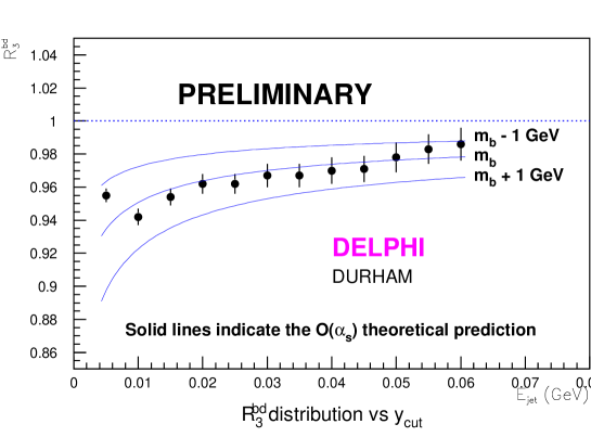
Figure 8. Preliminary experimental results for the ratio $R_{3}^{bd}$ from DELPHI Collaboration.

Taking as the theoretical uncertainty for the running bottom quark mass at $m_{Z}$ half of the difference from the $\mu=m_{Z}/2$ and $\mu=2\>m_{Z}$ predictions we find as expected the smallest uncertainty correspond to the DURHAM algorithm, $\Delta\bar{m}_{b}\simeq 110(MeV)$. JADE and EM share the same behaviour, $\Delta\bar{m}_{b}\simeq 130(MeV)$, slightly bigger than in the DURHAM case. Finally, the E algorithm grows to $\Delta\bar{m}_{b}\simeq 220(MeV)$. Case we enlarge the lower limit on $\mu$ we get for $\mu=m_{Z}/10$, $\Delta\bar{m}_{b}\simeq 250$, $300$ and $500(MeV)$ respectively.

3. Discussion and conclusions

In this thesis we have analyzed at NLO the quark mass dependence of the three-jet observable

$$R^{bd}_{3}=\frac{\Gamma^{b}_{3j}(y_{c})/\Gamma^{b}}{\Gamma^{d}_{3j}(y_{c})/\Gamma^{d}}~{},$$

for different jet clustering algorithms such as EM, JADE, E and DURHAM. In particular, we have studied the possibility of extracting the bottom quark mass from $R^{bd}_{3}$ at LEP.

Since quarks are not free particles the study of its mass needs a precise theoretical framework and, in fact, they should be treated more like coupling constants. The two most commonly used quark mass definitions are the perturbative pole mass and the $\overline{MS}$ scheme running mass. We reviewed in Chapter 1 some of the most recent determinations of all the quark masses, in particular, the bottom quark mass extracted from the bottomia spectrum from QCD Sum Rules and Lattice calculations. The bottom quark perturbative pole mass appeared to be around $M_{b}=4.6-4.7(GeV)$ whereas the running mass at the running mass scale read $\bar{m}_{b}(\bar{m}_{b})=(4.33\pm 0.06)GeV$. We analized its running until the $Z$-boson mass scale and we found $\bar{m}_{b}(m_{Z})=(3.00\pm 0.12)GeV$.

Since for the bottom quark the difference between the perturbative pole mass and the running mass at the $m_{Z}$ scale is quite significant it is crucial to specify, in any theoretical perturbative prediction at $m_{Z}$, which mass should we use. In practice, this means we have to go up to NLO, where a renormalization scheme has to be chosen, if we want to extract a meaningful value for the bottom quark mass, since the LO does not allow to distinguish among the different quark mass definitions.

We have explored a new method: the study of three-jet observables at LEP, different from QCD Sum Rules and Lattice calculations, for determining the bottom quark mass. Among other advantages, it would allow to extract the bottom quark mass far from threshold, in contrast to the other methods described above.

From our calculation, we have estimated, by exploring the $\mu$-dependence of our prediction at $m_{Z}$, a theoretical bottom quark mass uncertainty of at most $250(MeV)$ in the DURHAM algorithm, $300(MeV)$ for JADE and EM and $500(MeV)$ for the E algorithm. The preliminary experimental bottom quark mass uncertainty from the DELPHI Collaboration [60], see figure 8, in the DURHAM algorithm is expected to be $300(MeV)$. Nevertheless, that is not the last word but the first step. The experimental error would be improved, specially once the four experiments at LEP are taken into account, and we are still discussing how to improve the theoretical error. Resummed expressions would probably give a better result.

Therefore, even if, for the moment, this method can not be considered competitive with QCD Sum Rules and Lattice predictions, a total error of $300(MeV)$ in the DURHAM algorithm, slightly bigger in JADE and EM algorithm, should be enough to check, for the first time, how the bottom quark mass evolves, from low scales $\mu\sim 5(GeV)$ to the $m_{Z}$ scale, following the Renormalization Group prediction, in the same way the running of the strong coupling constant has been checked before.

Among other applications, our calculation would provide a better understanding of the systematic errors in the measurement of $\alpha_{s}(m_{Z})$ from $b\bar{b}$-production at LEP from the ratio of three to two jets [130] and therefore a better measurement of the strong coupling constant $\alpha_{s}^{b}(m_{Z})$.

Furthermore, quark mass effects are expected to be quite more important in top production at NLC (Next Linear Collider) and our calculation would be of a great interest.

In this thesis, we have concentrated in the study of the three-jet observable $R^{bd}_{3}$ ratio. To do that, we had to calculate the NLO matrix elements for the decay of the $Z$-boson into massive quarks. Main problem of such calculation was, in addition to UV divergences, the appearance of IR singularities. We were able first, by simple graphical arguments, to classify our transition amplitudes into different groups such that IR singularities cancel independently and second to build matrix elements free of singularities since we exclude from the phase space the IR region where integration is performed analytically. Once the IR behaviour is under control, it would be possible to build, with our matrix elements, a Monte Carlo generator opening the door to the study of other kind of three-jet observables (angular distributions, differential cross sections, etc $\ldots$ ) where massive quarks are involved. Furthermore, the two-jet decay rate can be extracted by subtracting from the well known total decay rate the three- and the, full infrared finite, four-jet decay rates. Therefore, the study of two-jet observables is also possible from our calculation.

Concluding, in a previous paper [25], we raised the question of the possibility of measuring the $b$-quark mass at LEP by using three-jet observables. In close collaboration with the DELPHI experimental group at Valencia [60], we have developed the necessary theoretical tools in order to extract a meaningful value for the $b$-quark mass from LEP data, in particular, the NLO calculation of the three-jet decay rate of the $Z$-boson into massive quarks. Clearly, more work has to be done but the effort is worth since it will allow for an independent measurement of $m_{b}$, far from threshold, and it will provide a test of the QCD Renormalization Group predictions.

Chapter 6 Loop integrals

We present in this appendix all the scalar one loop integrals we encountered in the calculation of the diagrams of figure 1. Since we are just interested in the interference transition probabilities of these diagrams with the born amplitudes we will only need the real part of such n-point scalar one loop integrals. Although we don’t specify it, the following results refer, in almost all the cases, just to the real part of these functions.

Appendix 6.A One- and two-point functions

One- and two-point one loop functions are defined in $D$ dimensions as

(6.1) $$\begin{split}&\frac{i}{16\pi^{2}}A(m)=\mu^{4-D}\int\frac{d^{D}k}{(2\pi)^{D}}\frac{1}{k^{2}-m^{2}}~{},\\ &\frac{i}{16\pi^{2}}B_{0}(p^{2},m_{1}^{2},m_{2}^{2})=\mu^{4-D}\int\frac{d^{D}k}{(2\pi)^{D}}\frac{1}{[k^{2}-m_{1}^{2}][(k-p)^{2}-m_{2}^{2}]}~{}.\\ \end{split}$$

They are the source of UV divergences.

For the scalar one-point integral in $D=4-2\epsilon$ dimensions we have the following result

(6.2) $$A(m)=m^{2}(\Delta-\log\frac{m^{2}}{\mu^{2}}+1)~{},$$

with

(6.3) $$\Delta=\frac{1}{\epsilon}-\gamma+\log 4\pi~{}.$$

the UV pole while for the two point functions we get

$$B_{0}(m_{b}^{2},0,m_{b}^{2}) = \>\Delta-\log\frac{m_{b}^{2}}{\mu^{2}}+2~{},$$

$$B_{0}(0,m_{b}^{2},m_{b}^{2}) = \>\Delta-\log\frac{m_{b}^{2}}{\mu^{2}}~{},$$

(6.4) $$B_{0}(0,0,m_{b}^{2}) = \>\Delta-\log\frac{m_{b}^{2}}{\mu^{2}}+1~{},$$

$$B_{0}(p_{13}^{2},0,m_{b}^{2}) = \>\Delta-\log\frac{m_{b}^{2}}{\mu^{2}}-\frac{y_{13}}{r_{b}+y_{13}}\log\frac{y_{13}}{r_{b}}+2~{},$$

$$B_{0}(s,m_{b}^{2},m_{b}^{2}) = \>\Delta-\log\frac{m_{b}^{2}}{\mu^{2}}+\beta\log c+2~{},$$

$$B_{0}(p_{12}^{2},m_{b}^{2},m_{b}^{2}) = \>\Delta-\log\frac{m_{b}^{2}}{\mu^{2}}+\beta_{12}\log c_{12}+2~{},$$

$$B_{0}(0,0,0) = \>0~{},$$

where

$$r_{b} =m_{b}^{2}/m_{Z}^{2}~{}, y_{ij}=2(p_{i}\cdot p_{j})/m_{Z}^{2}$$

(6.5) $$\beta =\sqrt{1-4r_{b}}~{}, \beta_{12}=\sqrt{1-4\frac{r_{b}}{y_{12}+2r_{b}}}~{},$$

$$c =\frac{1-\beta}{1+\beta}~{}, c_{12}=\frac{1-\beta_{12}}{1+\beta_{12}}~{}.$$

We have set to zero the $B_{0}(0,0,0)$ integral. Strictly speaking that is not completely true. On analyzing this integral in detail we encounter it receives contributions in terms of UV and IR divergences separately, i.e., we should write

(6.6) $$B_{0}(0,0,0)=\mu^{4-D}\int\frac{d^{D}k}{(2\pi)^{D}}\frac{1}{k^{4}}=\frac{1}{\epsilon_{UV}}-\frac{1}{\epsilon_{IR}}~{}.$$

If we try to distinguish between UV and IR poles we have to keep them. Since this kind of integrals just change the label of the divergences but not the number of poles in $1/\epsilon$ we will identify $\epsilon_{IR}=\epsilon_{UV}$. We can try to follow the origin of the UV and IR poles but we don’t gain nothing. Ultraviolet singularities are cancelled by the renormalization procedure that is very well known.

Appendix 6.B Three-point functions

The scalar three-point integral reads

(6.7) $$\frac{i}{16\pi^{2}}C_{0}(A,B,C,m_{1}^{2},m_{2}^{2},m_{3}^{2})=\\ \mu^{4-D}\int\frac{d^{D}k}{(2\pi)^{D}}\frac{1}{[k^{2}-m_{1}^{2}][(k+p_{1})^{2}-m_{2}^{2}][(k+p_{2})^{2}-m_{3}^{2}]}$$

where $A=p_{1}^{2}$, $B=(p_{1}-p_{2})^{2}$ and $C=p_{2}^{2}$. After Feynman parametrization and momentum integration we get

(6.8) $$C_{0}(A,B,C,m_{1}^{2},m_{2}^{2},m_{3}^{2})=\\ -\left(\frac{4\pi\mu^{2}}{q^{2}}\right)^{\frac{4-D}{2}}\Gamma\left(3-\frac{D}{2}\right)\int_{0}^{1}dx\int_{0}^{x}dy\frac{1}{(ax^{2}+by^{2}+cxy+dx+ey+f)^{3-\frac{D}{2}}}~{},\\$$

where

(6.9) $$\begin{split}a&=C~{},\\ b&=B~{},\\ c&=A-B-C~{},\\ d&=m_{3}^{2}-m_{1}^{2}-C~{},\\ e&=m_{2}^{2}-m_{3}^{2}+C-A~{},\\ f&=m_{1}^{2}-i\eta~{}.\end{split}$$

For $A$, $B$ and $C$ different from zero and if the scalar three-point function does not contain infrared divergences the integral can be performed in $D=4$ dimensions and can be expressed as a sum over twelve dilogarithms [77]

(6.10) $$C_{0}=\frac{1}{\sqrt{\lambda}}\sum_{i=1}^{3}\sum_{j=1}^{2}(-1)^{i}\left\{Li_{2}\left(\frac{x_{i}}{x_{i}-y_{ij}}\right)-Li_{2}\left(\frac{x_{i}-1}{x_{i}-y_{ij}}\right)\right\}~{},$$

with the Spence function or dilogarithm function defined as [113]

(6.11) $$Li_{2}(z)=-\int_{0}^{z}dt\frac{\log(1-t)}{t}~{},$$

and

(6.12) $$\begin{split}x_{1}&=-\frac{d+2a+(c+e)\alpha}{\sqrt{\lambda}}~{},\\ x_{2}&=-\frac{d+e\alpha}{(1-\alpha)\sqrt{\lambda}}~{},\\ x_{3}&=\frac{d+e\alpha}{\alpha\sqrt{\lambda}}~{},\\ y_{1j}&=\frac{-(c+e)\pm\sqrt{(c+e)^{2}-4b(a+d+f)}}{2b}~{},\\ y_{2j}&=\frac{-(d+e)\pm\sqrt{(d+e)^{2}-4f(a+b+c)}}{2(a+b+c)}~{},\\ y_{3j}&=\frac{-d\pm\sqrt{d^{2}-4af}}{2a}~{},\end{split}$$

where $\alpha$ is a real solution of the equation

(6.13) $$b\alpha^{2}+c\alpha+a=0~{},$$

and $\sqrt{\lambda}=c+2\alpha b$.

We define the following one loop integrals

(6.14) $$\begin{split}\frac{i}{16\pi^{2}}C01(y_{13})&=\mu^{4-D}\int\frac{d^{D}k}{(2\pi)^{D}}\frac{1}{k^{2}[(k+p_{13})^{2}-m_{b}^{2}][(k-p_{2})^{2}-m_{b}^{2}]}~{},\\ &\\ \frac{i}{16\pi^{2}}C02(y_{13})&=\mu^{4-D}\int\frac{d^{D}k}{(2\pi)^{D}}\frac{1}{k^{2}[(k+p_{13})^{2}-m_{b}^{2}][(k+p_{1})^{2}-m_{b}^{2}]}~{},\\ &\\ \frac{i}{16\pi^{2}}C03(y_{13})&=\mu^{4-D}\int\frac{d^{D}k}{(2\pi)^{D}}\frac{1}{k^{2}(k-p_{3})^{2}[(k+p_{1})^{2}-m_{b}^{2}]}~{},\\ &\\ \frac{i}{16\pi^{2}}C04(y_{12})&=\mu^{4-D}\int\frac{d^{D}k}{(2\pi)^{D}}\frac{1}{[k^{2}-m_{b}^{2}][(k+q)^{2}-m_{b}^{2}][(k+p_{12})^{2}-m_{b}^{2}]}~{},\\ &\\ \frac{i}{16\pi^{2}}C05(y_{12})&=\mu^{4-D}\int\frac{d^{D}k}{(2\pi)^{D}}\frac{1}{k^{2}[(k+p_{1})^{2}-m_{b}^{2}][(k-p_{2})^{2}-m_{b}^{2}]}~{}.\end{split}$$

For integral $C01$ we can apply directly Eq. (6.10) and take just its real part. For $C02$ and $C04$ we can calculate them either directly from the Feynman parametrization (LABEL:C0feynman) or from Eq. (6.10) by taking the appropriate limit. At the end we get a quite simplified result 

(6.15) $$\begin{split}C02(y_{13})&=\frac{1}{y_{13}}\left[\frac{1}{2}\log^{2}(A)+Li_{2}(A)-\frac{\pi^{2}}{6}\right]~{},\\ &\\ C04(y_{12})&=\frac{1}{1-(y_{12}+2r_{b})}\frac{1}{2}\left[\log^{2}c-\log^{2}c_{12}\right]~{},\end{split}$$

with $A=r_{b}/(r_{b}+y_{13})$. The three-point functions $C03$ and $C05$ are IR divergent and therefore we can not apply the general result of Eq. (6.10). In these two cases we obtain, after integration in $D=4-2\epsilon$ dimensions 

(6.16) $$C03(y_{13})=\frac{(4\pi)^{\epsilon}}{\Gamma(1-\epsilon)}\frac{1}{y_{13}}\left[\frac{1}{2\epsilon^{2}}+\frac{1}{2\epsilon}\log\frac{r_{b}}{y_{13}^{2}}\right.\\ \left.+\frac{1}{4}\log^{2}\frac{r_{b}}{y_{13}^{2}}-\frac{1}{2}\log^{2}A-Li_{2}(A)-\frac{7\pi^{2}}{12}\right]~{},$$

(6.17) $$C05(y_{12})=\frac{(4\pi)^{\epsilon}}{\Gamma(1-\epsilon)}\frac{1}{(y_{12}+2r_{b})\beta_{12}}\left[\left(\frac{1}{\epsilon}-\log r_{b}\right)\log c_{12}-2L(y_{12})\right]~{}.$$

where

(6.18) $$L(y_{12})=Li_{2}(c_{12})+\frac{\pi^{2}}{3}+\log(1-c_{12})\log c_{12}-\frac{1}{4}\log^{2}c_{12}~{}.$$

Appendix 6.C Four-point functions

In our one loop matrix elements we encounter the following four-point functions

(6.19) $$\frac{i}{16\pi^{2}}D05(y_{13},y_{12})=\\ \mu^{4-D}\int\frac{d^{D}k}{(2\pi)^{D}}\frac{1}{k^{2}[(k+p_{1})^{2}-m_{b}^{2}][(k+p_{13})^{2}-m_{b}^{2}][(k-p_{2})^{2}-m_{b}^{2}]}~{},$$

(6.20) $$\frac{i}{16\pi^{2}}D06(y_{13},y_{23})=\\ \mu^{4-D}\int\frac{d^{D}k}{(2\pi)^{D}}\frac{1}{k^{2}(k+p_{3})^{2}[(k+p_{13})^{2}-m_{b}^{2}][(k-p_{2})^{2}-m_{b}^{2}]}~{}.$$

Both four-point functions are IR divergent. The integral $D05$ has simple poles in $1/\epsilon$ while $D06$ presents double poles. To get their finite part is not an easy task but in order to extract the divergent piece we just need to split its non on-shell propagator.

For $D05$ we can write

(6.21) $$\frac{1}{(k+p_{13})^{2}-m_{b}^{2}}=\frac{1}{p_{13}^{2}-m_{b}^{2}}-\frac{k^{2}+2k\cdot p_{13}}{(p_{13}^{2}-m_{b}^{2})[(k+p_{13})^{2}-m_{b}^{2}]}~{}.$$

The IR divergence is isolated in the first term of the righthand side of the previous equation and give rise to $C05(y_{12})/y_{13}$. The other term generates two IR finite one loop integrals.

For $D06$ things are more complex. The splitting of the non on-shell propagator does not give directly the divergent piece due to the presence of IR double poles. First of all we have to notice $D06$ is invariant under the interchange of particles 1 and 2, i.e., the result of the integral should be symmetric in the two momenta invariants $y_{13}$ and $y_{23}$. We found the proper way for extracting the IR piece is as follows

(6.22) $$D06(y_{13},y_{23})=\frac{1}{y_{13}}C03(y_{23})+\frac{1}{y_{23}}C03(y_{13})+\mbox{\rm finite terms}~{}.$$

We leave for a future publication the detailed calculation of the finite contributions of the box one-loop integrals $D05$ and $D06$.

Appendix 6.D Explicit calculation of $C03$

For the $C03$ function a Feynman parametrization, (LABEL:C0feynman), with both Feynman parameters running from $0$ to $1$ is more convenient because the two integrals decouple each other

(6.23) $$C03=-(4\pi)^{\epsilon}\Gamma(1+\epsilon)\int_{0}^{1}x^{-1-2\epsilon}dx\\ \int_{0}^{1}\left[(r_{b}+y_{13})y^{2}-(2r_{b}+y_{13})y+r_{b}-i\eta\right]^{-1-\epsilon}dy~{}.$$

The integral over the x-parameter is immediate and we left just with

(6.24) $$C03=(4\pi)^{\epsilon}\frac{\Gamma(1+\epsilon)}{2\epsilon}(r_{b}+y_{13})^{-1-\epsilon}\int_{0}^{1}(1-y)^{-1-\epsilon}(y_{0}-y)^{-1-\epsilon}dy~{},$$

where $y_{0}$ is the root of the y-parameter polynomial. The last integral gives rise to an Hypergeometric function

(6.25) $$C03=\frac{(4\pi)^{\epsilon}}{\Gamma(1-\epsilon)}\frac{\Gamma(1+\epsilon)\Gamma(-\epsilon)}{2\epsilon}\\ (r_{b}+y_{13})^{-1-\epsilon}y_{0}^{-1-\epsilon}{}_{2}F_{1}[1+\epsilon,1,1-\epsilon,\frac{1}{y_{0}}]~{},$$

that with the help of some mathematical properties [3, 115] can be written in terms of a dilogarithm function [113, 46]

(6.26) $$\begin{split}{}_{2}F_{1}[1+\epsilon,1,1-\epsilon,\frac{1}{y_{0}}]&=\left(1-\frac{1}{y_{0}}\right)^{-1-2\epsilon}{}_{2}F_{1}[-2\epsilon,-e,1-\epsilon,\frac{1}{y_{0}}]\\ &=\left(1-\frac{1}{y_{0}}\right)^{-1-2\epsilon}\left[1+2\epsilon^{2}Li_{2}\left(\frac{1}{y_{0}}\right)+O(\epsilon^{3})\right]~{}.\end{split}$$

In the region of physical interest $y_{0}=r_{b}/(r_{b}+y_{13})$ is smaller than one and we should perform an analytic continuation taking into account the $-i\eta$ prescription. The final result is quoted in Eq. (6.16).

Appendix 6.E Passarino-Veltman reduction

We illustrate here a simple example of how to reduce vectorial and tensorial loop integrals [114] to the scalar one loop functions defined in the previous sections. Let’s consider the following set of integrals

(6.27) $$\mu^{4-D}\int\frac{d^{D}k}{(2\pi)^{D}}\frac{k_{\mu};k_{\mu}k_{\nu}}{k^{2}[(k+p_{1})^{2}-m_{b}^{2}][(k-p_{2})^{2}-m_{b}^{2}]}=\frac{i}{16\pi^{2}}C0_{\mu;\mu\nu}~{}.$$

By Lorentz invariance

(6.28) $$\begin{split}C0^{\mu}\>\>&=p_{1}^{\mu}C_{11}+p_{2}^{\mu}C_{12}~{},\\ C0^{\mu\nu}&=g^{\mu\nu}C_{20}+p_{1}^{\mu}p_{1}^{\nu}C_{21}+p_{2}^{\mu}p_{2}^{\nu}C_{22}\\ &+(p_{1}^{\mu}p_{2}^{\nu}+p_{1}^{\nu}p_{2}^{\mu})C_{23}~{}.\end{split}$$

Now, we have to perform all the possible contractions with external momenta to extract the coefficients $C_{ij}$.

Let’s try with

(6.29) $$\mu^{4-D}\int\frac{d^{D}k}{(2\pi)^{D}}\frac{(k\cdot p_{1})}{k^{2}[(k+p_{1})^{2}-m_{b}^{2}][(k-p_{2})^{2}-m_{b}^{2}]}=\\ \frac{i}{16\pi^{2}}\left[p_{1}^{2}C_{11}+(p_{1}\cdot p_{2})C_{12}\right]~{}.$$

The scalar product in the numerator can be written, including the on-shell condition $p_{1}^{2}=m_{b}^{2}$, as

(6.30) $$2(k\cdot p_{1})=(k+p_{1})^{2}-k^{2}-p_{1}^{2}=[(k+p_{1})^{2}-m_{b}^{2}]-k^{2}~{}.$$

Therefore, our initial vectorial three propagators integral reduces automatically to the sum of two scalar two-point functions

(6.31) $$\mu^{4-D}\int\frac{d^{D}k}{(2\pi)^{D}}\frac{2(k\cdot p_{1})}{k^{2}[(k+p_{1})^{2}-m_{b}^{2}][(k-p_{2})^{2}-m_{b}^{2}]}=\\ \mu^{4-D}\int\frac{d^{D}k}{(2\pi)^{D}}\left[\frac{1}{k^{2}[(k-p_{2})^{2}-m_{b}^{2}]}-\frac{1}{[(k+p_{1})^{2}-m_{b}^{2}][(k-p_{2})^{2}-m_{b}^{2}]}\right]$$

(6.32) $$=\frac{i}{16\pi^{2}}\left[B_{0}(p_{2}^{2},0,m_{b}^{2})-B_{0}(p_{12}^{2},m_{b}^{2},m_{b}^{2})\right]~{}.$$

Same argument can be applied to the scalar product with $p_{2}$. In this simple case the final result is as follows

(6.33) $$C_{11}=-C_{12}=\frac{1}{y_{12}-2r_{b}}\left[B_{0}(p_{12}^{2},m_{b}^{2},m_{b}^{2})-B_{0}(m_{b}^{2},0,m_{b}^{2})\right]~{}.$$

To reduce the tensorial integrals to scalar integrals we have to follow the same mathematical procedure. Solutions appear to be quite more complex, specially when we have to treat with box integrals, i.e., one loop integrals with four propagators. To solve all the Pasarino-Veltman reductions we needed we have used the FeynCalc 1.0 [107, 45] algebraic package for Mathematica 2.0. whereas all the Dirac algebra was performed with HIP [78].

Appendix 6.F The problem of $\gamma_{5}$ in $D$-dimensions

Multi-loop calculations with dimensional regularization often encounter the question of how to treat $\gamma_{5}$ in $D$ dimensions. Occasionally the problem can be circumvented by exploiting chiral symmetry. In our case, in the limit of massless quarks axial and vector contributions to the three jets decay rate of the $Z$ boson should be equal. In general, however, a consistent definition must be formulated.

A rigourous choice based on the original definition of ’t Hooft and Veltman [76]

(6.34) $$\gamma_{5}=\frac{i}{4!}\epsilon_{\mu\nu\rho\sigma}\gamma^{\mu}\gamma^{\nu}\gamma^{\rho}\gamma^{\sigma}~{}.$$

can be found in [29]. As a consequence of the lost of anticommuntativity of $\gamma_{5}$ in this new definition, standard properties of the axial current as well as the Ward identities are violated. In particular, extra finite renormalization constant should be introduced to restore the correctly renormalized non-singlet axial current..

Nevertheless, it has been checked [30] that for diagrams with an even number of $\gamma_{5}$ connected to the external current the treatment based on a naïve anticommutating $\gamma_{5}$ leads to the same answer. This is our case because for unpolarized final state quarks only terms proportional to the square of the vector and axial-vector neutral current couplings survive. Therefore, in our approach we have restricted to work with anticommutating $\gamma_{5}$ avoiding extra complications.

Chapter 7 Phase space in $D=4-2\epsilon$ dimensions

The phase space for $n$-particles in the final state in $D$-dimensions [64, 102, 103] $(D=4-2\epsilon)$ has the following general form

(7.1) $$\begin{split}dPS(n)&=(2\pi)^{D}\prod_{i=1,n}\frac{d^{D-1}p_{i}}{(2\pi)^{D-1}2E_{i}}\delta^{D}\left(q-\sum_{i=1,n}p_{i}\right)\\ &=(2\pi)^{D}\prod_{i=1,n}\frac{d^{D}p_{i}}{(2\pi)^{D-1}}\delta(p_{i}^{2}-m_{i}^{2})\Theta(E_{i})\delta^{D}\left(q-\sum_{i=1,n}p_{i}\right)~{}.\end{split}$$

Then doing several trivial integrations we have the following phase-space factor for the process $Z\rightarrow b\bar{b}$

(7.2) $$PS(2)=\frac{1}{4\pi}\frac{\beta}{2}\frac{\Gamma(1-\epsilon)}{\Gamma(2-2\epsilon)}{\left(\frac{\beta^{2}m_{Z}^{2}}{4\pi}\right)}^{-\epsilon}~{},$$

where $\beta=\sqrt{1-4r_{b}}$ with $r_{b}=m_{b}^{2}/m_{Z}^{2}$,

For the case of the decay into three particles, $Z\rightarrow b(p_{1})\bar{b}(p_{2})g(p_{3})$, we get

(7.3) $$PS(3)=\frac{m_{Z}^{2}}{16(2\pi)^{3}}\frac{1}{\Gamma(2-2\epsilon)}{\left(\frac{m_{Z}^{2}}{4\pi}\right)}^{-2\epsilon}\int\theta(h_{p})h_{p}^{-\epsilon}dy_{13}dy_{23}~{},$$

where the function $h_{p}$ which gives the phase-space boundary in terms of variables $y_{13}=2(p_{1}\cdot p_{3})/m_{Z}^{2}$ and $y_{23}=2(p_{2}\cdot p_{3})/m_{Z}^{2}$ has the form

(7.4) $$h_{p}=y_{13}y_{23}(1-y_{13}-y_{23})-r_{b}(y_{13}+y_{23})^{2}~{}.$$

Appendix 7.A System 1-3

For those four parton transitions amplitudes of the process $Z\rightarrow b(p_{1})+\bar{b}(p_{2})+g(p_{3})+g(p_{4})$ containing the denominator $y_{13}=2(p_{1}\cdot p_{3})/m_{Z}^{2}$, i.e., with gluon labelled as 3 soft, it is convenient to write the four-body phase space as a quasi three body decay

(7.5) $$\begin{split}q\rightarrow&p_{13}+p_{2}+p_{4}\\ &\hookrightarrow p_{1}+p_{3}~{}.\end{split}$$

Figure 1. Threemomenta in the c.m. frame of particles 1 and 3.

We will refer to this as the “1-3 system” [55]. In the c.m. frame of particles 1 and 3 the four-momenta can be written as

(7.6) $$\begin{split}p_{1}&=(E_{1},\ldots,\mbox{\rm\bf p}_{1}\sin\theta\cos\theta^{\prime},\mbox{\rm\bf p}_{1}\cos\theta)~{},\\ p_{2}&=(E_{2},\ldots,0,\mbox{\rm\bf p}_{2})~{},\\ p_{3}&=E_{3}(1,\ldots,-\sin\theta\cos\theta^{\prime},-\cos\theta)~{},\\ p_{4}&=E_{4}(1,\ldots,\sin\beta,\cos\beta)~{},\end{split}$$

where the dots in $p_{1}$ and $p_{3}$ indicate $D-3$ unspecified, equal and opposite angles (in $D$ dimensions) and $D-3$ zeros in $p_{2}$ and $p_{4}$. In terms of variables

(7.7) $$y_{13}=\frac{2(p_{1}\cdot p_{3})}{m_{Z}^{2}}~{},\qquad y_{123}=\frac{2(p_{2}\cdot p_{13})}{m_{Z}^{2}}~{},\qquad y_{134}=\frac{2(p_{4}\cdot p_{13})}{m_{Z}^{2}}~{},$$

with $p_{13}=p_{1}+p_{3}$, energies and threemomenta read ($s=m_{Z}^{2}=1$)

$$E_{1} =\frac{y_{13}+2r_{b}}{2\sqrt{y_{13}+r_{b}}}~{}, \mbox{\rm\bf p}_{1}=\frac{y_{13}}{2\sqrt{y_{13}+r_{b}}}~{},$$

(7.8) $$E_{2} =\frac{y_{123}}{2\sqrt{y_{13}+r_{b}}}~{}, \mbox{\rm\bf p}_{2}=\frac{1}{2\sqrt{y_{13}+r_{b}}}\sqrt{y_{123}^{2}-4r_{b}(y_{13}+r_{b})}~{},$$

$$E_{3} =\frac{y_{13}}{2\sqrt{y_{13}+r_{b}}}~{}, E_{4}=\frac{y_{134}}{2\sqrt{y_{13}+r_{b}}}~{}.$$

Setting $v=\frac{1}{2}(1-\cos\theta)$, we obtain for the $D$-dimensional phase space in this system

(7.9) $$\begin{split}PS(4)&=\frac{m_{Z}^{2}}{16(2\pi)^{3}}\frac{1}{\Gamma(2-2\epsilon)}{\left(\frac{m_{Z}^{2}}{4\pi}\right)}^{-2\epsilon}\int dy_{134}dy_{234}\\ &m_{Z}^{2(1-\epsilon)}\frac{S}{16\pi^{2}}\frac{(4\pi)^{\epsilon}}{\Gamma(1-\epsilon)}\int dy_{13}\theta(h_{p})h_{p}^{-\epsilon}\frac{y_{13}^{1-2\epsilon}}{(y_{13}+r_{b})^{1-\epsilon}}\\ &\int_{0}^{1}dv(v(1-v))^{-\epsilon}\frac{1}{N_{\theta^{\prime}}}\int_{0}^{\pi}d\theta^{\prime}\sin^{-2\epsilon}\theta^{\prime}~{},\end{split}$$

where $S=1/2!$ is the statistical factor, $N_{\theta^{\prime}}$ is a normalization factor determined such that

(7.10) $$\int_{0}^{\pi}d\theta^{\prime}\sin^{-2\epsilon}\theta^{\prime}=N_{\theta^{\prime}}=2^{2\epsilon}\pi\frac{\displaystyle\Gamma(1-2\epsilon)}{\displaystyle\Gamma^{2}(1-\epsilon)}~{},$$

and the function

(7.11) $$\begin{split}h_{p}&=y_{123}y_{134}(1-y_{123}-y_{134})\\ &+r_{b}\left(-1+2(y_{123}+y_{134})-(y_{123}^{2}+4y_{123}y_{134}+2y_{134}^{2})\right)\\ &+4r_{b}^{2}(1-y_{123}-y_{134})-4r_{b}^{3}\\ &+\left(-1+6r_{b}-8r_{b}^{2}\right.\\ &\qquad\left.+2(1-3r_{b})(y_{123}+y_{134})-y_{123}^{2}-3y_{123}y_{134}-y_{134}^{2}\right)y_{13}\\ &+\left(2-5r_{b}-2y_{123}-2y_{134}\right)y_{13}^{2}-y_{13}^{3}~{},\end{split}$$

defines the limits of the phase space.

Appendix 7.B System 3-4

For diagrams containing the denominator $y_{34}=2(p_{3}\cdot p_{4})/m_{Z}^{2}$, that is, gluons labelled as 3 and 4 soft and/or collinear we will work in the c.m. frame of both gluons where

(7.12) $$\begin{split}p_{1}&=(E_{1},\ldots,0,\mbox{\rm\bf p}_{1})~{},\\ p_{2}&=(E_{2},\ldots,\mbox{\rm\bf p}_{2}\sin\beta,\mbox{\rm\bf p}_{2}\cos\beta)~{},\\ p_{3}&=E_{3}(1,\ldots,\sin\theta\cos\theta^{\prime},\cos\theta)~{},\\ p_{4}&=E_{4}(1,\ldots,-\sin\theta\cos\theta^{\prime},-\cos\theta)~{}.\end{split}$$

Figure 2. Threemomenta in the c.m. frame of particles 3 and 4.

In this case we will use the following set of variables

(7.13) $$y_{34}=\frac{2(p_{3}\cdot p_{4})}{m_{Z}^{2}}~{},\qquad y_{134}=\frac{2(p_{1}\cdot p_{34})}{m_{Z}^{2}}~{},\qquad y_{234}=\frac{2(p_{2}\cdot p_{34})}{m_{Z}^{2}}~{},$$

with $p_{34}=p_{3}+p_{4}$, in terms of which energies and threemomenta read

$$E_{1} =\frac{y_{134}}{2\sqrt{y_{34}}}~{}, \mbox{\rm\bf p}_{1}=\frac{1}{2\sqrt{y_{34}}}\sqrt{y_{134}^{2}-4r_{b}y_{34}}~{},$$

(7.14) $$E_{2} =\frac{y_{234}}{2\sqrt{y_{34}}}~{}, \mbox{\rm\bf p}_{2}=\frac{1}{2\sqrt{y_{34}}}\sqrt{y_{234}^{2}-4r_{b}y_{34}}~{},$$

$$E_{3} =\frac{\sqrt{y_{34}}}{2}~{}, E_{4}=\frac{\sqrt{y_{34}}}{2}~{}.$$

We obtain for the $D$-dimensional phase space in this system

(7.15) $$\begin{split}PS(4)&=\frac{m_{Z}^{2}}{16(2\pi)^{3}}\frac{1}{\Gamma(2-2\epsilon)}{\left(\frac{m_{Z}^{2}}{4\pi}\right)}^{-2\epsilon}\int dy_{134}dy_{234}\\ &m_{Z}^{2(1-\epsilon)}\frac{S}{16\pi^{2}}\frac{(4\pi)^{\epsilon}}{\Gamma(1-\epsilon)}\int dy_{34}\theta(h_{p})h_{p}^{-\epsilon}y_{34}^{-\epsilon}\\ &\int_{0}^{1}dv(v(1-v))^{-\epsilon}\frac{1}{N_{\theta^{\prime}}}\int_{0}^{\pi}d\theta^{\prime}\sin^{-2\epsilon}\theta^{\prime}~{},\end{split}$$

with

(7.16) $$\begin{split}h_{p}&=y_{134}y_{234}(1-y_{134}-y_{234})-r_{b}(y_{134}+y_{234})^{2}\\ &+\left(-1+4r_{b}+2(1-2r_{b})(y_{134}+y_{234})-y_{134}^{2}-3y_{134}y_{234}-y_{234}^{2}\right)y_{34}\\ &+2(1-2r_{b}-y_{134}-y_{234})y_{34}^{2}-y_{34}^{3}~{}.\end{split}$$

Observe $h_{p}$ reduce to (7.4) in the case $y_{34}\rightarrow 0$. Furthermore, in this limit $p_{34}=p_{3}+p_{4}$ behaves as the momentum of a pseudo on-shell gluon because $p_{34}^{2}\rightarrow 0$.

Index

• $\alpha_{s}(m_{Z})$ §1
  • world average Chapter 1
• $\alpha_{s}^{b}(m_{Z})$ Chapter 2
• Angular distribution §4
• Beta function Chapter 1
• Bloch-Nordsiek theorem Chapter 4, Chapter 5, §1
• Bubble diagram Chapter 4, Figure 1
• C01 Appendix 6.B
• C02 Appendix 6.B
• C03 Appendix 6.B, Appendix 6.C, Appendix 6.D
• C04 Appendix 6.B
• C05 Appendix 6.B, Appendix 6.C
• $c_{A}$ §3
• CDF Chapter 1, Chapter 1
• $C_{F}$ §1
• Chiral Perturbation Theory Chapter 1
• Chiral symmetry Chapter 2, Appendix 6.F, §3
• Class A Chapter 4, §1, §1, §2, §2
• Class B Chapter 4, §1, §1, §1, §2, §2
• Class C §2.2, §2, §2, §2
• Class D §3
• Class E §3, §3
• Class F §3, §3
• Class G §2.2, §2.2
• Cutkowsky rules §2, §3
• $c_{V}$ §3
• D05 Appendix 6.C
• D06 Appendix 6.C
• Decoupling Chapter 1
• DELPHI Figure 8, §2, Figure 3, §3
• Dilogarithm function Appendix 6.B, Appendix 6.D, §2.1
• Dimensional Regularization Chapter 3, Chapter 3, §1, §2.2
• DØ Chapter 1, Chapter 1
• DURHAM algorithm §2
• E algorithm §2
• Effective Theory Chapter 1
• EM algorithm §2, §4
• ERT §1
• Exponentiation §2
• Fermi statistics §3
• FERMILAB Chapter 1
• FeynCalc Appendix 6.E
• Feynman
  • gauge Chapter 3, §1
  • parameters Chapter 5
  • parametrization Appendix 6.B, Appendix 6.B, Appendix 6.D, §1
• Flavour universality Chapter 2
• Four-point function Appendix 6.C
• Furry’s theorem §3
• Gamma function Chapter 1
• $\gamma_{5}$ Chapter 3, Appendix 6.F
• Generator §3
• Ghosts §2
• Gluon
  • bremsstrahlung §1
  • mass footnote 1, Chapter 3
  • selfenergy Chapter 4, §2.2, §3
  • three gluon vertex footnote 1, Chapter 3, Figure 1, §2
• $\gamma-Z$-interference §3.2
• Hadronization §2, §2, §2
• Higgs Chapter 1
• HIP Chapter 3, Appendix 6.E
• $h_{p}$ Appendix 7.A, Appendix 7.B, Chapter 7
• HQET Chapter 1
• Hypergeometric function Appendix 6.D, §2.1
• Inclusive decay rate Chapter 2, §1
• IR singularities §1
  • collinear Chapter 4, §1, §2, §2
  • soft Chapter 4, §1, §1
• JADE algorithm §2
  • $A^{(0)}(y_{c})$ function §3
• Jet
  • clustering algorithms §2
  • resolution parameter Chapter 2, §2
• Kinoshita-Lee-Nauenberg theorem Chapter 4, Chapter 5, §1
• $\Lambda_{QCD}$ Chapter 1
• Lattice Chapter 1, Chapter 2
• LEP Chapter 2, Chapter 2, Chapter 3, §3.2
• Lorentz invariance Appendix 6.E
• Matching conditions Chapter 1
• Mathematica Chapter 3, Appendix 6.E
• Monte Carlo Chapter 2, Chapter 5, §1, §2, §3, §4
• Neutral current
  • axial-vector coupling §1
  • vector coupling §1
• NLC §3
• Non-perturbative effects Chapter 2
• Non-singlet axial current Appendix 6.F
• $N_{\theta^{\prime}}$ Appendix 7.A
• One-point function Appendix 6.A
• Parton item 2, §2
• Passarino-Veltman reduction Appendix 6.E, §1
• Phase space Chapter 7
• PS(2) Chapter 7
• PS(3) Chapter 7
• PS(4) Appendix 7.A, Appendix 7.B
• QCD §1
• QED footnote 1
  • initial-state radiation §3.2
  • radiator §3.2
• Quark mass
  • Euclidean Chapter 1
  • perturbative pole Chapter 1, §1, §4
  • running Chapter 1, §1, §4
• $R_{3}^{bd}$ Chapter 3, §1.2, §2.1, §2.1, §2, §2, §2, §3, §3.1, §3, §4
• Renormalization
  • Group Equations Chapter 1
  • scheme
    • $\overline{MS}$ Chapter 1, Chapter 1, §1, §1
    • on-shell §1
• Renormalon Chapter 1
• Riemann zeta-function Chapter 1
• Singlet contributions §3
• Slicing method Chapter 5
• Spence function Appendix 6.B
• Spontaneous symmetry breaking Chapter 2
• Standard Model Chapter 1, Chapter 2, §1.1
• Subtraction method Chapter 5
• Sum Rules Chapter 1, Chapter 2
• System 1-3 Appendix 7.A
• System 3-4 Appendix 7.B
• T0 Chapter 4, Figure 1, §1
• T1 Chapter 4, §1
• T2 Chapter 4, §1
• T3 Chapter 4, §1
• T4 Chapter 4, §1
• T5 Chapter 4, §1
• T6 Chapter 4, §1
• Tensor one-loop integrals Appendix 6.E
• Three-jet decay rate §3
• Threshold Chapter 1, Chapter 1, Chapter 1, Chapter 1, Chapter 1
• Top quark Chapter 1, §3
• $T_{R}$ §3
• Triangle anomaly footnote 5
• Two-point function Appendix 6.A
• Unification Chapter 1, Chapter 2
• UV divergences Chapter 4, Chapter 5, Appendix 6.A, Appendix 6.A, §1
• Vector one-loop integrals Appendix 6.E
• VEGAS Chapter 5
• Ward identities Chapter 3, Appendix 6.F
• $y_{13}$ Appendix 7.A
• $y_{34}$ Appendix 7.B
• Yukawa coupling Chapter 1, Chapter 2

Agradecimientos

Quisiera agradecer, en primer lugar, a mi director de tesis por los consejos recibidos durante estos años, por haberse involucrado en este largo y pesado cálculo en algunos momentos clave de su desarrollo y por haberme corregido incluso el mal inglés de esta tesis.

Me gustaría agradecer al grupo experimental de DELPHI en Valencia el apoyo moral recibido, el haber acogido a “el teórico” en sus viajes por la Helvetia y el soporte técnico e informático sin el cual esta tesis no habría podido ser realizada.

Mi profundo agradecimiento a todos los miembros del Departamento de Física Teórica, en particular a aquellos que en algún momento se interesaron por el estado del cálculo e intentaron ayudarme y muy especialmente a la Asociación de Becarios “Juan Valdés” por las horas que desahogo que supuso la visita periódica al bar de la Facultad.

Por último, quisiera agradecer a mis amigos de siempre simplemente el haber continuado ahí y a mis padres, hermanas, abuela y a Chelo por haberme aguantado tanto cuando lo único que me preocupaba eran los quarks y los gluones.

References

- [1] S. Abachi et al., Observation of the top quark, Phys.Rev.Lett. 74 (1995), 2632–2637, DØ Collaboration.
- [2] F. Abe et al., Observation of top quark production in collisions, Phys.Rev.Lett. 74 (1995), 2626–2631, CDF Collaboration.
- [3] M. Abramowitz and I. A. Stegun, Handbook of mathematical functions, Dover, New York, 1972.
- [4] P. Abreu et al., Determination of for b quarks at the Z0 resonance, Phys.Lett. B307 (1993), 221, DELPHI Collaboration.
- [5] C. Adami, E. G. Drukarev, and B. L. Ioffe, Isospin violation in QCD sum rules for baryons, Phys.Rev. D48 (1993), 2304.
- [6] B. Adeva et al., Measurement of the strong coupling constant for bottom quarks at the Z0 resonance, Phys.Lett. B271 (1991), 461–467, L3 Collaboration.
- [7] R. Akers et al., A test of the flavor independence of the strong interaction for five flavors, Z.Phys. C60 (1993), 397–420, OPAL Collaboration.
- [8] A. A. Akhundov, D. Yu. Bardin, and T. Riemann, Electroweak one loop corrections to the decay of the neutral vector boson, Nucl.Phys. B276 (1986), 1.
- [9] C. R. Allton et al., Quark masses from lattice QCD at the next-to-leading order, Nucl.Phys. B431 (1994), 667–685.
- [10] A. B. Arbuzov, D. Yu. Bardin, and A. Leike, Analytic final state corrections with cut for massive fermions, Mod.Phys.Lett. A7 (1992), 2029–2038. Erratum, ibid. A9 (1994)1515.
- [11] F. Aversa, M. Greco, P. Chiappetta, and J. P. Guillet, Jet inclusive production to : Comparison with data, Phys.Rev.Lett. 65 (1990), 401–403.
- [12] H. Baer, J. Ohnemus, and J. F. Owens, A next-to-leading logarithm calculation of jet photoproduction, Phys.Rev. D40 (1989), 2844.
- [13] A. Ballestrero, E. Maina, and S. Moretti, Heavy quark production at colliders in three and four jet events, Phys.Lett. B294 (1992), 425–430.
- [14] by same author, Heavy quarks and leptons at colliders, Nucl.Phys. B415 (1994), 265–292.
- [15] W. Bartels et al., Z.Phys. C33 (1986), 23, JADE Collaboration.
- [16] W. Beenakker and W. Hollik, The width of the Z boson, Z.Phys. C40 (1988), 141.
- [17] F. A. Berends, W. L. van Neerven, and G. J. H. Burgers, Higher order radiative corrections at LEP energies, Nucl.Phys. B297 (1988), 429. Erratum, Nucl. Phys. B304 (1988) 921.
- [18] J. Bernabéu, A. Pich, and A. Santamaria, : A signature of hard mass terms for a heavy top, Phys.Lett. 200B (1988), 569.
- [19] by same author, Top quark mass from radiative corrections to the decay, Nucl.Phys. B363 (1991), 326–344.
- [20] W. Bernreuther, Decoupling of heavy quarks in quantum chromodynamics, Ann.Phys. 151 (1983), 127.
- [21] W. Bernreuther and W. Wetzel, Decoupling of heavy quarks in the minimal subtraction scheme, Nucl.Phys. B197 (1982), 228.
- [22] S. Bethke, Proceedings of the High-energy Physics International Euroconference on Quantum Chromodynamics (QCD 96), Montpellier, France, 4-12 Jul 1996.
- [23] S. Bethke, Z. Kunszt, D. E. Soper, and W. J. Stirling, New jet cluster algorithms: Next-to-leading order QCD and hadronization corrections, Nucl.Phys. B370 (1992), 310–334.
- [24] J. Bijnens, J. Prades, and E. de Rafael, Light quark masses in QCD, Phys.Lett. B348 (1995), 226–238.
- [25] M. Bilenkii, G. Rodrigo, and A. Santamaria, Three jet production at LEP and the bottom quark mass, Nucl.Phys. B439 (1995), 505–535.
- [26] F. Bloch and A. Nordsieck, Phys.Rev. 52 (1937), 54.
- [27] by same author, Note on the radiation field of the electron, Phys.Rev. 52 (1937), 54–59.
- [28] A. I. Bochkarev and R. S. Willey, On the scheme dependence of the electroweak radiative corrections, Phys.Rev. D51 (1995), 2049–2052.
- [29] P. Breitenlohner and D. Maison, Dimensional renormalization and the action principle, Commun.Math.Phys. 52 (1977), 11.
- [30] D. J. Broadhurst and A. L. Kataev, Connections between deep inelastic and annihilation processes at next to next-to-leading order and beyond, Phys.Lett. B315 (1993), 179–187.
- [31] N. Brown and W. Stirling, Finding jets and summing soft gluons: A new algorithm, Z.Phys. C53 (1992), 629–636.
- [32] D. Buskulic et al., Test of the flavor independence of , Phys.Lett. B355 (1995), 381–393, ALEPH Collaboration.
- [33] S. Catani, Yu. L. Dokshitser, M. Olsson, G. Turnock, and B. R. Webber, New clustering algorithm for multi - jet cross-sections in annihilation, Phys.Lett. B269 (1991), 432–438.
- [34] S. Catani and M. H. Seymour, A general algorithm for calculating jet cross sections in NLO QCD, hep-ph/9605323.
- [35] T. H. Chang, K. J. F. Gaemers, and W. L. van Neerven, QCD corrections to the mass and width of the intermediate vector bosons, Nucl.Phys. B202 (1982), 407.
- [36] K. G. Chetyrkin, C. A. Dominguez, D. Pirjol, and K. Schilcher, Mass singularities in light quark correlators: The strange quark case, Phys.Rev. D51 (1995), 5090–5100.
- [37] K. G. Chetyrkin, S. G. Gorishny, and F. V. Tkachov, Operator product expansion in the minimal subtraction scheme, Phys.Lett. 119B (1982), 407.
- [38] K. G. Chetyrkin and J. H. Kühn, Mass corrections to the Z decay rate, Phys.Lett. B248 (1990), 359–364.
- [39] K. G. Chetyrkin, J. H. Kühn, and A. Kwiatkowski, QCD corrections to the cross-section and the Z boson decay rate, hep-ph/9503396.
- [40] K. G. Chetyrkin and A. Kwiatkowski, Complete mass corrections of order to the axial Z boson decay rate in the large top mass limit, Phys.Lett. B305 (1993), 285–294.
- [41] J. Chrin, Proc. of the 28th Rencontre de Moriond, Les Arcs, Savoie, France, March 1993 (J. Trän Thanh Van, ed.), 1993, p. 313.
- [42] M. Crisafulli, V. Giménez, G. Martinelli, and C. T. Sachrajda, First lattice calculation of the B meson binding and kinetic energies, Nucl.Phys. B457 (1995), 594–620.
- [43] C. T. H. Davies et al., A new determination of using lattice QCD, Phys.Rev.Lett. 73 (1994), 2654–2657.
- [44] by same author, A precise determination of from lattice QCD, Phys.Lett. B345 (1995), 42–48.
- [45] A. Denner, Techniques for calculation of electroweak radiative corrections at the one loop level and results for w physics at LEP200, Fortschr.Phys. 41 (1993), 307–420.
- [46] A. Devoto and D. W. Duke, Table of integrals and formulae for feynman diagram calculations, Riv.Nuovo Cim.7,no. 6 (1984), 1.
- [47] A. Djouadi, J. H. Kühn, and P. M. Zerwas, b jet asymmetries in Z decays, Z.Phys. C46 (1990), 411–418.
- [48] C. A. Dominguez, Heavy quark masses from QCD sum rules, hep-ph/9410362.
- [49] C. A. Dominguez, G. R. Gluckman, and N. Paver, Mass of the charm quark from QCD sum rules, Phys.Lett. B333 (1994), 184–189.
- [50] C. A. Dominguez and N. Paver, New determination of the beauty quark mass, Phys.Lett. B293 (1992), 197–200.
- [51] J. F. Donoghue, B. R. Holstein, and D. Wyler, Electromagnetic selfenergies of pseudoscalar mesons and dashen’s theorem, Phys.Rev. D47 (1993), 2089–2097.
- [52] by same author, Mass ratios of the light quarks, Phys.Rev.Lett. 69 (1993), 3444.
- [53] A. X. El-Khadra and B. P. Mertens, The heavy quark masses from quarkonia, hep-lat/9501022.
- [54] V. L. Eletskii and B. L. Ioffe, Estimates of and from QCD sum rules for and isospin mass differences, Phys.Rev. D48 (1993), 1441.
- [55] R. K. Ellis, D. A. Ross, and A. E. Terrano, The perturbative calculation of jet structure in annihilation, Nucl.Phys. B178 (1981), 421.
- [56] S. D. Ellis, Z. Kunszt, and D. E. Soper, The one jet inclusive cross-section at order . 1. gluons only, Phys.Rev. D40 (1989), 2188.
- [57] K. Fabricius, I. Schmitt, G. Kramer, and G. Schierholz, Higher order perturbative QCD calculation of jet cross- sections in annihilation, Zeit.Phys. C11 (1981), 315.
- [58] S. Frixione, Z. Kunszt, and A. Signer, Three-jet cross sections to next-to-leading order, Nucl.Phys. B467 (1996), 399–442.
- [59] J. Fuster, Recent results on QCD at LEP, Proc. XXII International Meeting on Fundamental Physics, Jaca, Spain. (1994).
- [60] J. Fuster, S. Cabrera, and S. Martí, Experimental studies of QCD using flavour tagged jets with DELPHI, Proceedings of the High-energy Physics International Euroconference on Quantum Chromodynamics (QCD 96), Montpellier, France, 4-12 Jul 1996. hep-ex/9609004.
- [61] J. Gasser and H. Leutwyler, Chiral perturbation theory: Expansions in the mass of the strange quark, Nucl.Phys. B250 (1985), 465.
- [62] by same author, to one loop, Nucl.Phys. B250 (1985), 539.
- [63] by same author, Low-energy expansion of meson form-factors, Nucl.Phys. B250 (1985), 517.
- [64] R. Gastmans, J. Verwaest, and R. Meuldermans, Dimensional regularization in massless qed, Nucl.Phys. B105 (1976), 454.
- [65] D. Gerdes, Top quark physics results from CDF and D0, Presented at 1996 DPF / DPB Summer Study on New Directions for High-energy Physics (Snowmass 96), Snowmass, CO, 25 Jun - 12 Jul 1996. hep-ex/9609013. FERMILAB Conf-96/342-E., CDF Collaboration.
- [66] W. T. Giele and E. W. N. Glover, Higher order corrections to jet cross-sections in annihilation, Phys.Rev. D46 (1992), 1980–2010.
- [67] W. T. Giele, E. W. N. Glover, and David A. Kosower, Higher order corrections to jet cross-sections in hadron colliders, Nucl.Phys. B403 (1993), 633–670.
- [68] V. Giménez, G. Martinelli, and C. T. Sachrajda, A high statistics lattice calculation of the b-meson binding energy, hep-lat/9607018.
- [69] E. W. N. Glover, R. Kleiss, and J. J. van der Bij, The decay of the Z boson into four massive fermions, Z.Phys. C47 (1990), 435–448.
- [70] N. Gray, D. J. Broadhurst, W. Grafe, and K. Schilcher, Three loop relation of quark and pole masses, Z.Phys. C48 (1990), 673–680.
- [71] G. Grunberg, Y. J. Ng, and S. H. H. Tye, Angular distributions of heavy quark jets in annihilation, Phys.Rev. D21 (1980), 62.
- [72] F. Gutbrod, G. Kramer, and G. Schierholz, Higher order QCD corrections to the three jet cross- sections: Bare versus dressed jets, Z.Phys. C21 (1984), 235.
- [73] K. Hagiwara, T. Kuruma, and Y. Yamada, Three jet distributions from the one loop vertex at colliders, Nucl.Phys. B358 (1991), 80–96.
- [74] R. Harlander, M. Jezabek, J. H. Kühn, and T. Teubner, Polarization in top quark pair production near threshold, Phys. Lett. B346 (1995), 137–142.
- [75] R. Hempfling and B. A. Kniehl, On the relation between the fermion pole mass and yukawa coupling in the standard model, Phys.Rev. D51 (1995), 1386–1394.
- [76] G. ’t Hooft and M. Veltman, Regularization and renormalization of gauge fields, Nucl.Phys. B44 (1972), 189.
- [77] by same author, Scalar one loop integrals, Nucl.Phys. B153 (1979), 365–401.
- [78] A. Hsieh and E. Yehudai, HIP: Symbolic high-energy physics calculations, Comput.Phys. 6 (1992), 253–261.
- [79] B. L. Ioffe, Associated production of gluonic jets and heavy mesons in annihilation, Phys.Lett. 78B (1978), 277.
- [80] M. Jamin and M. Münz, The strange quark mass from QCD sum rules, Z.Phys. C66 (1995), 633–646.
- [81] J. Jersák, E. Laermann, and P. M. Zerwas, Electroweak production of heavy quarks in annihilation, Phys.Rev. D25 (1982), 1218. Erratum, Phys. Rev. D36 (1987) 310.
- [82] T. Kinoshita, J. Math. Phys. 3 (1962), 650.
- [83] by same author, Mass singularities of feynman amplitudes, J.Math.Phys. 3 (1962), 650–677.
- [84] J. G. Körner and G. Schuler, Complete amplitude and cross-section structure of one loop contributions to , Z.Phys. C26 (1985), 559.
- [85] G. Kramer and B. Lampe, Integrals for two loop calculations in massless QCD, J.Math.Phys. 28 (1987), 945.
- [86] by same author, Two jet cross-section in annihilation, Z.Phys. C34 (1987), 497.
- [87] by same author, Jet cross-sections in annihilation, Fortschr.Phys. 37 (1989), 161.
- [88] G. Kramer, G. Schierholz, and J. Willrodt, Cross-sections and angular distributions of three jet final states in annihilation for heavy quarks, Z.Phys. C4 (1980), 149.
- [89] J. H. Kühn and P. M. Zerwas, The toponium scenario, Phys.Rept. 167 (1988), 321.
- [90] Z. Kunszt, From scattering amplitudes to cross sections in QCD, Lecture presented at the Theoretical Advanced Study Institute in ELementary Particle Physics (TASI 95): QCD and beyond, Boulder, CO, June 4-30, 1995. hep-ph/9603235.
- [91] Z. Kunszt, P. Nason, G. Marchesini, and B. R. Webber, QCD at LEP, Proceedings of the 1989 LEP Physics Workshop, Geneva, Swizterland, Feb 20, 1989.
- [92] Z. Kunszt and D. E. Soper, Calculation of jet cross-sections in hadron collisions at order , Phys.Rev. D46 (1992), 192–221.
- [93] E. Laermann and P. M. Zerwas, Hard gluon bremsstrahlung off heavy quarks in annihilation, Phys.Lett. 89B (1980), 225.
- [94] P. Langacker and N. Polonsky, The bottom mass prediction in supersymmetric grand unification: Uncertainties and constraints, Phys.Rev. D49 (1994), 1454–1467.
- [95] S. A. Larin, T. van Ritbergen, and J. A. M. Vermaseren, The large quark mass expansion of hadrons) and + hadrons) in the order , Nucl.Phys. B438 (1995), 278–306.
- [96] T. D. Lee and M. Nauenberg, Degenerate systems and mass singularities, Phys.Rev. 133 (1964), B1549.
- [97] T.D. Lee and M. Nauenberg, Phys.Rev. B133 (1964), 1549.
- [98] S. Leone, Top quark results at CDF, Proceedings of the High-energy Physics International Euroconference on Quantum Chromodynamics (QCD 96), Montpellier, France, 4-12 Jul 1996., CDF Collaboration.
- [99] G. P. Lepage, A new algorithm for adaptive multidimensional integration, J.Comput.Phys. 27 (1978), 192.
- [100] by same author, VEGAS: An adaptive multidimensional integration program, CLNS-80/447 (1980).
- [101] M. L. Mangano, P. Nason, and G. Ridolfi, Heavy quark correlations in hadron collisions at next-to- leading order, Nucl.Phys. B373 (1992), 295–345.
- [102] W. J. Marciano, Dimensional regularization and mass singularities, Phys.Rev. D12 (1975), 3861.
- [103] W. J. Marciano and A. Sirlin, Dimensional regularization of infrared divergences, Nucl.Phys. B88 (1975), 86.
- [104] S. Martí i García, Study of the energy dependence of the differences between quark and gluon jets using the DELPHI detector at LEP, Ph.D. thesis, Universitat de València, 1995. hep-ex/9511004.
- [105] G. Martinelli and C. T. Sachrajda, On the difficulty of computing higher-twist corrections., hep-ph/9605336.
- [106] A. Mendez and A. Pomarol, QCD corrections to the charged higgs boson hadronic width, Phys. Lett. B252 (1990), 461–466.
- [107] R. Mertig, M. Bohm, and A. Denner, FeynCalc: Computer algebraic calculation of feynman amplitudes, Comput.Phys.Commun. 64 (1990), 345.
- [108] S. Narison, Model independent determination of from -like inclusive decays in and implications for the -parameters, hep-ph/9504333.
- [109] by same author, A fresh look into the heavy quark mass values, Phys.Lett. B341 (1994), 73–83.
- [110] M. Neubert, Heavy quark masses, mixing angles, and spin flavor symmetry, hep-ph/9404296.
- [111] by same author, Heavy quark symmetry, Phys.Rept. 245 (1994), 259–396.
- [112] H. P. Nilles, Isolating gluon jets, Phys.Rev.Lett. 45 (1980), 319.
- [113] P. Pascual and R. Tarrach, QCD: Renormalization for the practitioner, Berlin, Germany: Springer, 277 P. ( Lecture Notes In Physics, 194), 1984.
- [114] G. Passarino and M. Veltman, One loop corrections for annihilation into in the weinberg model, Nucl.Phys. B160 (1979), 151.
- [115] Bateman Manuscript Project, Higher transcendental functions, McGraw-Hill, New York, 1953.
- [116] L. J. Reinders, H. Rubinstein, and S. Yazaki, Hadron properties from QCD sum rules, Phys.Rept. 127 (1985), 1.
- [117] L. J. Reinders, S. Yazaki, and H. R. Rubinstein, Two point functions for flavor changing currents in QCD, Phys.Lett. 103B (1981), 63.
- [118] T. G. Rizzo, Three jet final states in Z0 decay for heavy quarks, Phys.Rev. D22 (1980), 2213.
- [119] G. Rodrigo, Low-energy yukawa input parameters for yukawa coupling unification, Proceedings of the International Workshop on Elementary Particle Physics: Present and Future, Valencia, 5-9 Jun 1995, pp. 360-370. hep-ph/9507236.
- [120] by same author, Quark mass effects in QCD jets, Proceedings of the High-energy Physics International Euroconference on Quantum Chromodynamics (QCD 96), Montpellier, France, 4-12 Jul 1996. hep-ph/9609213.
- [121] G. Rodrigo and A. Santamaria, QCD matching conditions at thresholds, Phys.Lett. B313 (1993), 441–446.
- [122] G. A. Schuler and J. G. Körner, Oriented three jet events in annihilation, Nucl.Phys. B325 (1989), 557.
- [123] J. Schwinger, Particles, sources and fields, Addison-Wesley, Reading, Mass., 1973.
- [124] M. A. Shifman, A. I. Vainshtein, M. B. Voloshin, and V. I. Zakharov, puzzle in quantum chromodynamics, Phys.Lett. 77B (1978), 80.
- [125] G. Sterman and S. Weinberg, Jets from quantum chromodynamics, Phys.Rev.Lett. 39 (1977), 1436.
- [126] R. Tarrach, The pole mass in perturbative QCD, Nucl. Phys. B183 (1981), 384.
- [127] S. Titard and F. J. Yndurain, Rigorous QCD evaluation of spectrum and ground state properties of heavy systems: With a precision determination of , , Phys.Rev. D49 (1994), 6007–6025.
- [128] M. M. Tung, Order longitudinal spin polarization in heavy quark production, Phys.Rev. D52 (1995), 1353–1358.
- [129] M. M. Tung, J. Bernabéu, and J. Penarrocha, Analytic results for bottom and top quark production in collisions, Nucl.Phys. B470 (1996), 41–70.
- [130] J.A. Valls, Determinación de la constante de acoplamiento fuerte para quarks , , con el detector DELPHI en LEP, Ph.D. thesis, Universitat de València, 1994.
- [131] E. W. Varnes, Measurement of the top quark mass at D0, Presented at 1996 Annual Divisional Meeting (DPF 96) of the Division of Particles and Fields of the American Physical Society, Minneapolis, MN, 10-15 Aug 1996. FERMILAB Conf-96/243-E., DØ Collaboration.
- [132] Z. Was, Radiative corrections, Lectures given at the 1993 European School of High Energy Physics, Zakopane, Poland, 12-25 Sep 1993, CERN 94-04 (1994), 307.
Index
-
§1