Abstract

We investigate the observable consequences of creating cosmic texture by breaking a global SU(3) symmetry, rather than the SU(2) case which is generally studied. To this end, we study the nonlinear sigma model for a totally broken SU(3) symmetry, and develop a technique for numerically solving the classical field equations. This technique is applied in a cosmological context: the energy of the collapsing SU(3) texture field is used as a gravitational source for the production of perturbations in the primordial fluids of the early universe. From these calculations, we make predictions about the appearance of the anisotropies in the cosmic microwave background radiation (CMBR) which would be present if the large scale structure of the universe was gravitationally seeded by the collapse of SU(3) textures.

1 Introduction

Over the last few years, there has been a great deal of research on the effects of topological defects in the the early universe. In particular, one class of topological defect, textures, has emerged as an interesting canidate for creating the seeds of large scale structure in the early universe [1]. In three spatial dimensions, textures can be created in any symmetry breaking scheme where the vacuum manifold has a nontrivial third homotopy group, $\pi_{3}$. This situation is quite generic - for example if any nonabelian Lie group is completely broken, $\pi_{3}$ is nontrivial. There are a multitude of symmetry breaking schemes which could produce textures (a general classification has been given in [2]). But so far the only case which has been studied in any detail has been the simplest case, where the vacuum manifold is SU(2)${}\simeq{}\rm S^{3}$. An accurate nonlinear sigma model code has been developed for SU(2) textures al.[3], and it has been possible to extract detailed predictions of the power spectrum of inhomogeneities and nongaussianity of the CMBR anisotropies [3], [4].

In the light of such investigations, it is natural to ask whether the primary results from these simulations are particular to SU(2), or whether they are more general, pertaining to many or all field theories which would create texture. To answer this question, one must study the effects of textures that come from at least one other group. All simple Lie groups have a nontrivial $\pi_{3}$ so in principle one might choose any one of them. However, simplicity dictates SU(3) as the obvious choice. In this paper we shall study the effects of textures coming from a broken global SU(3) symmetry upon the CMBR anisotropies and density fluctuations of the early universe. A complementary investigation of more general texture theories has been recently conducted by Sornberger et. al. [5].

There is also some motivation from particle physics to study the effects of a totally broken global SU(3) symmetry. Joyce and Turok, [6], have pointed out that if the family symmetry among the quarks and leptons is broken by the Higgs mechanism, then we must have Higgs fields which totally break some three dimensional representation of a simple Lie Group. The only simple Lie groups which have three dimensional representations are SU(2) and SU(3). Joyce and Turok argue that SU(2) does not work well, as it does not easily break to make one quark family much more massive than the others, whereas in SU(3) this occurs naturally. A gauged SU(3) family symmetry would be anomolous, so such an SU(3) family symmetry must be global. When this symmetry is broken, the Goldstone modes of the Higgs fields would produce cosmic texture. In particle physics terms, the point of the present paper is to explore the cosmological consequences of a global SU(3) family symmetry broken at the GUT scale.

In this paper, a technique for studying textures from a broken global SU(3) symmetry is developed and applied, with the goal of making predictions about fluctuations in the cosmic microwave background. In section 2, we state the problem and derive the relevant nonlinear sigma model equations  [6]. In section 3, we develop a finite difference algorithm based upon these equations, and in section 4 we describe tests of the stability and accuracy of this algorithm. In section 5 we present some results about the scaling behavior of this algorithm, and the appearance of the CMBR fluctuations if the primordial density fluctuations of the universe come from this type of texture.

We find that the cosmological consequences of textures coming from a totally broken SU(3) symmetry are in most respects very similar to those from SU(2) textures. We present some preliminary evidence of differences in the shape of the CMBR anisotropy power spectrum, but more accurate techniques will be needed to fully resolve these.

2 Formulation of the problem

We wish to totally break the fundamental representation of SU(3) via the Higgs mechanism. In [6], Joyce and Turok describe this process in detail. In order to do this, our Higgs field must consist of two complex triplets, $\mbox{\boldmath$\Sigma$}^{1},\mbox{\boldmath$\Sigma$}^{2}\in{\rm C}^{3}$, which have a “Mexican hat” potential whose minimum is topologically equivalent to SU(3). Without loss of generality, one can choose these fields so that the minimum of the potential is described by:

$${\mbox{\boldmath$\Sigma$}^{1}}^{\dagger}\mbox{\boldmath$\Sigma$}^{1}=v_{1}^{2},\qquad{\mbox{\boldmath$\Sigma$}^{2}}^{\dagger}\mbox{\boldmath$\Sigma$}^{2}=v_{2}^{2},\qquad{\mbox{\boldmath$\Sigma$}^{1}}^{\dagger}\mbox{\boldmath$\Sigma$}^{2}=0\ .$$ (1)

Here $v_{1},v_{2}$ are the vacuum expectation values of $\mbox{\boldmath$\Sigma$}^{1},\mbox{\boldmath$\Sigma$}^{2}$, and are not necessarily equal to one another. (See equation (62) of [6].) Any particular set of $\mbox{\boldmath$\Sigma$}^{1},\mbox{\boldmath$\Sigma$}^{2}$ satisfying (1) clearly define a unique member of SU(3), for if we define

$$\mbox{\boldmath$\psi$}={\mbox{\boldmath$\Sigma$}^{1}\over v_{1}},\qquad\mbox{\boldmath$\chi$}={\mbox{\boldmath$\Sigma$}^{2}\over v_{2}},$$ (2)

then we can immediately construct an SU(3) group element, in the fundamental representation,

$$U=\left(\begin{array}[]{ccc}|&|&|\\ \mbox{\boldmath$\psi$}^{\dagger}\times\mbox{\boldmath$\chi$}^{\dagger}&\mbox{\boldmath$\psi$}&\mbox{\boldmath$\chi$}\\ |&|&|\end{array}\right)\ .$$ (3)

Note that the vacuum manifold is only identical to SU(3) geometrically if $v_{1}=v_{2}$. Otherwise it represents a ‘stretched’ version of SU(3).

We wish to construct a nonlinear sigma model which will describe the classical dynamics of these fields, assuming that they are restricted to this minimum.

The first thing we need are the classical field equations. The Lagrangian density for this system is

$${\cal L} = v_{1}^{2}\nabla_{\mu}\mbox{\boldmath$\psi$}^{\dagger}\nabla^{\mu}\mbox{\boldmath$\psi$}+v_{2}^{2}\nabla_{\mu}\mbox{\boldmath$\chi$}^{\dagger}\nabla^{\mu}\mbox{\boldmath$\chi$}+$$ (4)

$$\qquad\lambda_{\psi}(\mbox{\boldmath$\psi$}^{\dagger}\mbox{\boldmath$\psi$}-1)+\lambda_{\chi}(\mbox{\boldmath$\chi$}^{\dagger}\mbox{\boldmath$\chi$}-1)+\lambda_{\psi\chi}\mbox{\boldmath$\psi$}^{\dagger}\mbox{\boldmath$\chi$}+\lambda_{\psi\chi}^{*}\mbox{\boldmath$\chi$}^{\dagger}\psi\ ,$$

where the $\lambda$s are all Lagrange multipliers, with $\lambda_{\psi},\lambda_{\chi}$ real, and $\lambda_{\psi\chi}$ complex valued. Note that the theory has one free parameter, the ratio of VEVs of the two Higgs fields, $v_{1}/v_{2}$. Using this Lagrangian, we obtain classical field equations:

$$\nabla_{\mu}\nabla^{\mu}\mbox{\boldmath$\psi$}+(\nabla_{\mu}\mbox{\boldmath$\psi$}^{\dagger}\nabla^{\mu}\mbox{\boldmath$\psi$})\mbox{\boldmath$\psi$}+{2v_{2}^{2}\over v_{1}^{2}+v_{2}^{2}}(\nabla_{\mu}\mbox{\boldmath$\chi$}^{\dagger}\nabla^{\mu}\mbox{\boldmath$\psi$})\mbox{\boldmath$\chi$} = {\bf 0}\ ,$$

$$\nabla_{\mu}\nabla^{\mu}\mbox{\boldmath$\chi$}+(\nabla_{\mu}\mbox{\boldmath$\chi$}^{\dagger}\nabla^{\mu}\mbox{\boldmath$\chi$})\mbox{\boldmath$\chi$}+{2v_{1}^{2}\over v_{1}^{2}+v_{2}^{2}}(\nabla_{\mu}\mbox{\boldmath$\psi$}^{\dagger}\nabla^{\mu}\mbox{\boldmath$\chi$})\mbox{\boldmath$\psi$} = {\bf 0}\ .$$ (5)

(Compare equations (63) of [6].)

For cosmological purposes, we are interested in evolving very inhomogeneous field configurations, in regions where a texture is collapsing and the nonlinear terms in the equations are very important. There is little hope of making much progress analytically in general, and recourse to numerical techniques is needed.

We wish to discretize the field equations on a grid. However, any direct discretization of the field equations (5) will fail immediately and drastically: adding small corrections $\Delta\mbox{\boldmath$\psi$},\Delta\mbox{\boldmath$\chi$}$ according to a discrete version of (5) in general violates the sigma model constraints $|\mbox{\boldmath$\psi$}|^{2}=|\mbox{\boldmath$\chi$}|^{2}=1$, $\mbox{\boldmath$\psi$}^{\dagger}\mbox{\boldmath$\chi$}=0$. With those gone, the fields will no longer represent a member of SU(3), and the simulation becomes meaningless.

Interestingly, the standard method of dealing with this problem: to discretize the action and enforce the necessary constraints with a discrete set of Lagrange multipliers, does not work here. This is a pity, because this technique works beautifully for SU(2) (see Pen et al, [3], eqns (67) and (68)) and yields a very fast, efficient algorithm for evolving the SU(2) field forward. This method fails here because one must simultaneously solve for four Lagrange multipliers, ($\lambda_{\psi},\lambda_{\chi}$, and the real and imaginary components of $\lambda_{\psi\chi}$), at each spacetime point. One needs to solve four coupled nonlinear (quadratic) equations for four unknowns, at each point on the grid, at each timestep. (For SU(2), one only needs to solve single a quadratic equation.) This is numerically costly and complex - it must be done by iterative methods, and one has to worry about choosing the right one of the sixteen roots.

In order to solve the SU(3) field equations numerically, it is helpful to restate the problem in a form which more obviously respects the structure of the group. As written in (5), the field equations describe the motion of two three dimensional complex scalar fields. Thus there are twelve real degrees of freedom, which are four too many for describing a member of SU(3). We have to try to control the remaining four dimensions by imposing constraints in some clever fashion. It would be far better to work with a formulation of the field equations which only included the eight real degrees of freedom that exist in the problem.

Note that this problem of extra degrees of freedom has nothing to do with this being a field equation: the same problem would exist if we had only a single pair of complex 3-vectors, which were constrained to be of unit length and always perpendicular to one another. In fact, this is analogous to a very simple classical mechanical system. If the two vectors were real, instead of complex valued, then the single point system would have the same dynamics as a pair of iron bars, of unequal length, welded together perpendicular to one another, and with their point of contact held fixed, but otherwise free to rotate, as in figure 1. In this analogous system, the motion is trivial: there are three degrees of freedom, so the motion of this system is completely determined by conservation of angular momentum.

Figure 1: An analogous simple mechanical system.

The pair of bars conserves angular momentum because their Lagrangian is invariant under rotations in 3-space, SO(3). Going back to the SU(3) breaking Higgs field, the Lagrangian is clearly unchanged by an analogous global SU(3) rotation, $\mbox{\boldmath$\psi$}\rightarrow U\mbox{\boldmath$\psi$},\mbox{\boldmath$\chi$}\rightarrow U\mbox{\boldmath$\chi$}$. This invariance instantly gives us eight conserved Noether charges, components of angular momentum on this internal SU(3) space. Since our fields only have eight real degrees of freedom, their dynamics are entirely determined by the conservation of these Noether currents. Further, if we formulate the problem entirely in terms of the local member of SU(3), $U(x)$, and the local internal angular momentum densities, then it will be written entirely in terms of the eight real field degrees of freedom, and the corresponding velocities, with no extra degrees of freedom to be dealt with.

In terms of Noether currents, then, the field equations are

$$\nabla^{\mu}J^{a}_{\mu}=0\ ,$$ (6)

where the Noether currents $J^{a}_{\mu}$ are given by

$$J^{a}_{\mu}={\rm Im}\left\{v_{1}^{2}\mbox{\boldmath$\psi$}^{\dagger}T^{a}\partial_{\mu}\mbox{\boldmath$\psi$}+{}v_{2}^{2}\mbox{\boldmath$\chi$}^{\dagger}T^{a}\partial_{\mu}\mbox{\boldmath$\chi$}\right\}.$$ (7)

Here the $T^{a}$ are the generators of SU(3); for sake of convenience we will always use a basis where ${\rm Tr}[T^{a}T^{b}]=\delta^{ab}$. Here and below, we will use the convention that if $X^{a}$ are the components of a Lie algebra member, then $X=X^{a}T^{a}\in$ L(SU(3)) is the algebra element itself.

Now, define the local internal angular momentum densities, $L^{a}=J_{0}^{a}$. In a flat FRW universe, the field evolution equations, (6), become

$$\partial_{\tau}L^{a} = \partial_{i}J^{a}_{i}-2{\dot{a}\over a}L^{a}$$ (8)

$$= {\rm Im}\left\{v_{1}^{2}\mbox{\boldmath$\psi$}^{\dagger}T^{a}\nabla^{2}\mbox{\boldmath$\psi$}+{}v_{2}^{2}\mbox{\boldmath$\chi$}^{\dagger}T^{a}\nabla^{2}\mbox{\boldmath$\chi$}\right\}-2{\dot{a}\over a}L^{a}\ .$$

Here $g_{\mu\nu}=a^{2}(\tau){\rm diag}\{1,-1,-1,-1\}$, so $a(\tau)$ is the usual scale factor; we are working in conformal time and comoving spatial coordinates: we assume the background spacetime is flat Friedmann-Robertson-Walker. $\nabla^{2}$ is the ordinary flat space Laplacian. The ${\rm Im}\{\partial_{i}\mbox{\boldmath$\psi$}^{\dagger}T^{a}\partial_{i}\mbox{\boldmath$\psi$}\}$ terms have vanished from (8) because the hermiticity of $T^{a}$ makes the quantity in brackets purely real.

With equation (8), we have a straightforward, easily calculable method for evolving the angular momenta, $L$, forward provided we have the fields $\psi$ and $\chi$. In order to have a complete method of evolving the fields forward, we need to be able to evolve the SU(3) field forward, provided we know $L$. To go back to the mechanical analogy: we need to solve for angular velocity in terms of position and angular momentum; we need a moment of inertia tensor. Using the condensed notation of (3), we need $\partial_{\tau}U$. Now, since $U(x)$ must always remain upon the group, we know that there exists some $\Omega(x)\ \in$ L(SU(3)) such that

$$\partial_{\tau}U=i\Omega U\ ,$$ (9)

and we need to get $\Omega$ from $L$. The necessary transformation can be accomplished by taking the definition of $L$:

$$L^{a}=J_{0}^{a}={\rm Im}\left\{v_{1}^{2}\mbox{\boldmath$\psi$}^{\dagger}T^{a}\stackrel{{\scriptstyle\mbox{{\huge.}}}}{{\mbox{\boldmath$\psi$}}}+\ v_{2}^{2}\mbox{\boldmath$\chi$}^{\dagger}T^{a}\stackrel{{\scriptstyle\mbox{{\huge.}}}}{{\mbox{\boldmath$\chi$}}}\right\}\ ,$$ (10)

and constructing the quantities:

$$\mbox{\boldmath$\psi$}^{\dagger}L^{a}T^{a}\mbox{\boldmath$\psi$},\qquad\mbox{\boldmath$\psi$}^{\dagger}L^{a}T^{a}\mbox{\boldmath$\chi$},\qquad\mbox{\boldmath$\psi$}^{\dagger}L^{a}T^{a}(\mbox{\boldmath$\psi$}^{\dagger}\times\mbox{\boldmath$\chi$}^{\dagger})\ ,\qquad\mbox{etc.}$$ (11)

These components may be evaluated, to solve for $\stackrel{{\scriptstyle\mbox{{\huge.}}}}{{\mbox{\boldmath$\psi$}}},\stackrel{{\scriptstyle\mbox{{\huge.}}}}{{\mbox{\boldmath$\chi$}}}$, by using the following general relation: For any complex 3-vectors, $A,B,C$,

$${\rm Im}\left[A^{\dagger}T^{a}B\right]T^{a}C={1\over 2}i\left[\left(B^{\dagger}C\right)A-\left(A^{\dagger}C\right)B+{1\over 3}\left(B^{\dagger}A-A^{\dagger}B\right)C\right]\ ,$$ (12)

a kind of complex generalization of the BAC-CAB rule for double cross products. Equation (12) may be readily proven by writing $A^{\dagger}T^{a}B={\rm Tr}\left[T^{a}BA^{\dagger}\right]$, and then using the various known properties of the $T^{a}$s.

Using (12), then, we can evaluate the nine quantities of (11), and solve for $\Omega$. If we temporarily rotate coordinates so that $U=1$, then if we write

$$L=\left(\begin{array}[]{ccc}-L_{\psi\psi}-L_{\chi\chi}&L_{\alpha\psi}&L_{\alpha\chi}\\ L_{\alpha\psi}^{*}&L_{\psi\psi}&L_{\psi\chi}\\ L_{\alpha\chi}^{*}&L_{\psi\chi}^{*}&L_{\chi\chi}\end{array}\right)\ ,$$ (13)

(where $\alpha$ is a shorthand for $\mbox{\boldmath$\psi$}^{\dagger}\times\mbox{\boldmath$\chi$}^{\dagger}$), then $\Omega$ is

$$\Omega=2\left(\begin{array}[]{ccc}-\Omega_{\psi\psi}-\Omega_{\chi\chi}&{1\over v_{1}^{2}}L_{\alpha\psi}&{1\over v_{2}^{2}}L_{\alpha\chi}\\ {1\over v_{1}^{2}}L_{\alpha\psi}^{*}&{2L_{\psi\psi}+L_{\chi\chi}\over v_{1}^{2}}&\left({1\over v_{1}^{2}+v_{2}^{2}}L_{\psi\chi}\right)\\ {1\over v_{2}^{2}}L_{\alpha\chi}^{*}&\left({1\over v_{1}^{2}+v_{2}^{2}}\right)L_{\psi\chi}^{*}&{2L_{\chi\chi}+L_{\psi\psi}\over v_{2}^{2}}\end{array}\right)\ .$$ (14)

This can more be written more concisely as $\Omega^{a}={\bf I}^{a}_{\ b}L^{b}$, where ${\bf I}^{a}_{\ b}$ is the (almost diagonal) moment of inertia tensor, whose action is defined by (14).

Finally, (14) is only valid when $U=1$. In order to obtain the general relation, we must do and undo a rotation to the $U=1$ frame:

$$\Omega(L,U)=U\left\{{\bf I}\circ\left(U^{\dagger}LU\right)\right\}U^{\dagger}\ .$$ (15)

And that completes the circle. Taking (15),(14), (9), and (8) together, we have the field equations in a form where we have explicitly solved for the time derivatives of two fields, with no extra degrees of freedom. The equations upon which we will base the numerical field evolution are:

$$\stackrel{{\scriptstyle\mbox{{\huge.}}}}{{U}} = i\Omega(L,U)U\ ,$$ (16)

$$\stackrel{{\scriptstyle\mbox{{\huge.}}}}{{L^{a}}} = {\rm Im}\left\{v_{1}^{2}\mbox{\boldmath$\psi$}^{\dagger}T^{a}\nabla^{2}\mbox{\boldmath$\psi$}+v_{2}^{2}\mbox{\boldmath$\chi$}^{\dagger}T^{a}\nabla^{2}\mbox{\boldmath$\chi$}\right\}-2{\dot{a}\over a}L^{a}\ ,$$ (17)

where the precise form of $\Omega(L,U)$ is given by (15),(14).

3 The numerical algorithm

Now that we have the field equations, (16) and (17), we can set about constructing a field evolution algorithm based upon them. Space and time are discretized into grids. Since $U$ and $L$ are a field and its time variation, it is natural to place them on alternate half timesteps. We need to construct a finite difference technique for evolving each field forward, if the other is known one half timestep in the future.

3.1 Discrete evolution of $L$

One can read the algorithm for evolving $L$ forward directly from (17):

$$L^{a}_{n+1/2} = {a^{2}(\tau_{n-1/2})\over a^{2}(\tau_{n+1/2})}L^{a}_{n-1/2}$$ (18)

$$\quad+\ {\Delta_{\tau}\over\Delta_{x}^{2}}{\rm Im}\biggl{\{}v_{1}^{2}\mbox{\boldmath$\psi$}_{n}^{\dagger}T^{a}\left(\mbox{\boldmath$\psi$}^{i+1}_{n}+\mbox{\boldmath$\psi$}^{i-1}_{n}+...-6\mbox{\boldmath$\psi$}^{i,j,k}_{n}\right)$$

$$\qquad\qquad\qquad+\ v_{2}^{2}\mbox{\boldmath$\chi$}_{n}^{\dagger}T^{a}\Bigl{(}\mbox{\boldmath$\chi$}^{i+1}_{n}+\mbox{\boldmath$\chi$}^{i-1}_{n}+...-6\mbox{\boldmath$\chi$}^{i,j,k}_{n}\Bigr{)}\biggr{\}}\ ,$$

where the $...$ signify similar sums over nearest neighbors in the $j$ and $k$ directions. Here and elsewhere, if spatial indices are omitted, the $(i,j,k)^{\rm th}$ point is implied. The spatial derivatives piece of (18) is clearly second order accurate, and the factor $\left({a^{2}(\tau_{n-1/2})\over a^{2}(\tau_{n+1/2})}\right)$ takes the effect of the expansion of the universe into account: angular momentum density generically redshifts away with $a^{-2}$ as the universe expands. (That looks a little odd because we are in conformal time. In ordinary time, the angular momentum density would decay as $a^{-3}$, and integration over space with the proper volume element would give you a genuinely constant Noether charge.) Also, (18) has the pleasant property that it exactly conserves the total amount of each component of global angular momentum on the grid, since the sum over the entire grid of all of the discrete second spatial derivatives will be exactly zero (periodic boundary conditions are enforced).

And so we have eight Noether charges which are conserved in the continuum, and which are exactly conserved by this scheme of discretely evolving $L$ forward. Since this is only an exact global conservation, it says little about the accuracy of this method. (The local conservation of the internal angular momenta will only be correct to second order in $\Delta_{\tau}$, in general.) However, it does push heavily towards numerical stability, for it is more difficult for solutions of finite difference equations to diverge if they are required to separately conserve eight independent quantities while doing so.

3.2 Evolution equations for $U$

And so the evolution of the angular momentum field is well in hand. Next, we turn to the evolution of the SU(3) field, $U$. We would like to have a discrete version of the continuum equation, (16). The first requirement is that the evolution preserve the fact that $U\in$ SU(3), and so we want something like:

$$U_{n+1}=e^{i\Delta_{\tau}\Omega_{n+1/2}}U_{n}\ ,$$ (19)

which would be second order accurate in time, and would preserve SU(3) membership up to machine accuracy. However, in calculating (19), one immediately runs into a snag: the moment of inertia transformation from $L\rightarrow\Omega$ explicitly depends upon $U$. Thus, in order to calculate $\Omega_{n+1/2}$ we need a value for $U$ one half timestep into the future. So we need some kind of predictive method to get a value for $U_{n+1/2}$, at least first order accurate in $\Delta_{\tau}$.

Now, one can immediately think of several ways to construct such a thing: for example, one could approximate $U_{n+1/2}=\sqrt{U_{n}U_{n-1}^{\dagger}}\,U_{n}$. However, in this construction, as in all the rest, one is immediately confronted with ambiguities: is that last construction better, or worse, than taking $U_{n+1/2}=\sqrt{U_{n-1}^{\dagger}U_{n}}\,U_{n}$? Or should one try some kind of mean of the two? And there are a myriad of other possibilities, using the exponentials of combinations of $L_{n-1/2},L_{n+1/2}$, together with field values. These all have similar ordering ambiguities. The central problem is that constructions of the form (19) are trying to use group multiplication, instead of addition, to advance the fields. This is lovely, and keeps one on the group, but unfortunately in SU(3) group multiplication doesn’t commute. There will inevitably be ambiguities about the order in which the multiplication is to be done.

Instead of working on a group, and using multiplication, we should really work on a space in which addition is legal, and so no ambiguities of ordering can arise. The obvious such space is the Lie algebra: we should take the logarithm of the continuum equation (16), and discretize that instead. If we write

$$U(x)\equiv e^{iF(x)}\ ,\qquad F(x)\in\mbox{L(SU(3)),}$$ (20)

then (16) becomes:

$$\partial_{\tau}e^{iF}=i\Omega\left(L,e^{iF}\right)e^{iF}\ .$$ (21)

Now we need to solve (21) for $\stackrel{{\scriptstyle\mbox{{\huge.}}}}{{F}}$. This may be accomplished by means of the following construction (well known in lattice gauge theory):

$$i\Omega\ e^{iF} = \partial_{\tau}e^{iF}$$

$$e^{-iF}i\Omega\ e^{iF} = e^{-iF}\partial_{\tau}e^{iF}$$

$$= \int_{0}^{1}{{\rm d}\over{\rm d}\lambda}\left(e^{-i\lambda F}\partial_{\tau}e^{i\lambda F}\right){\,\rm d}\lambda$$

$$= \int_{0}^{1}\left[-iFe^{-i\lambda F}\partial_{\tau}e^{i\lambda F}+ie^{i\lambda F}\partial_{\tau}\left(Fe^{i\lambda F}\right)\right]{\,\rm d}\lambda$$

$$= \int_{0}^{1}\left[-iFe^{-i\lambda F}\partial_{\tau}e^{i\lambda F}+ie^{-i\lambda F}\stackrel{{\scriptstyle\mbox{{\huge.}}}}{{F}}e^{i\lambda F}+iFe^{-i\lambda F}\partial_{\tau}e^{i\lambda F}\right]{\,\rm d}\lambda$$

$$= \int_{0}^{1}ie^{-i\lambda{\rm Ad}\left[F\right]}\ \circ\stackrel{{\scriptstyle\mbox{{\huge.}}}}{{F}}{\,\rm d}\lambda\qquad\mbox{by the definition of adjoint,}$$

$$= i\left[\int_{0}^{1}e^{-i\lambda{\rm Ad}\left[F\right]}{\,\rm d}\lambda\right]\circ\stackrel{{\scriptstyle\mbox{{\huge.}}}}{{F}}$$

$$= i\left({e^{-i{\rm Ad}\left[F\right]}-1\over-i{\rm Ad}\left[F\right]}\right)\circ\stackrel{{\scriptstyle\mbox{{\huge.}}}}{{F}}$$

$$\stackrel{{\scriptstyle\mbox{{\huge.}}}}{{F}} = {-i{\rm Ad}\left[F\right]\over e^{-i{\rm Ad}\left[F\right]}-1}e^{-i{\rm Ad}\left[F\right]}\circ\Omega$$ (22)

$$= {i{\rm Ad}\left[F\right]\over e^{i{\rm Ad}\left[F\right]}-1}\circ\Omega\ .$$

And so we have an explicit expression for $\stackrel{{\scriptstyle\mbox{{\huge.}}}}{{F}}$ in terms of $\Omega$. Now, evaluation of (22) is little tricky, since the $8\times 8$ matrix $e^{i{\rm Ad}\left[F\right]}-1$ is singular, and (22) is written in terms of its inverse. There is no real problem, since the ${\rm Ad}\left[F\right]$ on top is also singular, and the two singularities cancel one another out. However, one cannot calculate the right hand side of (22) directly; one must interpret $\left({i{\rm Ad}\left[F\right]\over e^{i{\rm Ad}\left[F\right]}-1}\right)$ as the appropriate power series in $i{\rm Ad}\left[F\right]$. So long as the series converges, there is no ambiguity as to the meaning of (22).

We therefore have an expression for $\stackrel{{\scriptstyle\mbox{{\huge.}}}}{{F}}$, which can be expressed in terms of a power series we can find, of quantities that we know. At this point we could use a discrete version of (22), expressed as a power series, and attempt to construct a field evolution algorithm based upon that. That would be a sound way to proceed, but slow, as the power series may take many terms to converge. (Indeed, sometimes it doesn’t converge, as we discuss in appendix A.) Instead, with a little bit more maneuvering, we can construct an exactly calculable expression for the right hand side of (22).

We proceed as follows: Write out the power series expansion of (22),

$$\stackrel{{\scriptstyle\mbox{{\huge.}}}}{{F}} = \left[1+B_{1}i{\rm Ad}\left[F\right]+{B_{2}\over 2!}\left(i{\rm Ad}\left[F\right]\right)^{2}+{B_{3}\over 3!}\left(i{\rm Ad}\left[F\right]\right)^{3}+...\right]\circ\Omega$$ (23)

$$= \Omega+B_{1}i[F,\Omega]+{B_{2}i^{2}\over 2!}\left[F,[F,\Omega]\right]+{B_{3}i^{3}\over 3!}\left[F,\left[F,[F,\Omega]\right]\right]+...\ \ ,$$ (24)

by the definition of adjoint. Here the $B_{n}$ are the Bernoulli numbers. Now, diagonalize $F$,

$$F=RF_{D}R^{-1}\ ,\qquad\mbox{ and define }\Omega^{\prime}=R^{-1}\Omega R\ .$$ (25)

With these terms, the power series (24) becomes:

$$\stackrel{{\scriptstyle\mbox{{\huge.}}}}{{F}} = R\Omega^{\prime}R^{-1}+B_{1}i[RF_{D}R^{-1},R\Omega^{\prime}R^{-1}]$$ (26)

$$\qquad+{i^{2}B_{2}\over 2!}\left[RF_{D}R^{-1},[RF_{D}R^{-1},R\Omega^{\prime}R^{-1}]\right]+...$$

$$= R\biggl{\{}\Omega^{\prime}+iB_{1}[F_{D},\Omega^{\prime}]+{i^{2}B_{2}\over 2!}\left[F_{D},[F_{D},\Omega^{\prime}]\right]+...\biggr{\}}R^{-1}$$

Now, we can express $\Omega^{\prime}$ in terms of complexified Lie algebra elements (step operators):

$$\Omega^{\prime}=\Omega^{\prime}_{D}+\left(\Omega^{\prime}_{T}T_{+}+\Omega^{\prime}_{U}U_{+}+\Omega^{\prime}_{V}V_{+}+{\rm h.c.}\right)\ .$$ (27)

(The notation used here is standard for SU(3), see e.g. ref. [9] pp. 97–102. Also, we abbreviate $\Omega^{\prime}_{D}=\Omega^{\prime}_{T3}T_{3}+\Omega^{\prime}_{Y}Y$ is the diagonal part of $\Omega^{\prime}$. The components of $\Omega^{\prime}_{D}$ are purely real; the rest are complex.) Now, in the complexified basis of the Lie algebra, the commutator of a diagonal matrix with any basis element is proportional to that basis element. Thus we have a chain of identities of the form

$$\begin{array}[]{rcr}\mbox{$[\underbrace{F_{D},[F_{D},...[F_{D}}_{n\ {\rm terms}},T_{+}]]...]$}&=&\alpha_{{}_{T+}}^{n}T_{+}\ ,\end{array}$$ (28)

and similarly for all of the other basis elements. Here $\alpha_{{}_{T+}}(F_{D})$ is a simple real valued function of the diagonal components of $F_{D}$. Using these relations, we can write the power series as

$$\stackrel{{\scriptstyle\mbox{{\huge.}}}}{{F}} = R\biggl{\{}\left(1+B_{1}i\alpha_{{}_{T+}}+{B_{2}\over 2!}\left(i\alpha_{{}_{T+}}\right)^{2}+...\right)\Omega^{\prime}_{T+}T_{+}$$ (29)

$$\qquad\qquad+\ \mbox{ similar terms in other basis elements }\biggr{\}}R^{-1}\ .$$

And now we can explicitly resum the power series, which is now just a power series in an imaginary number. This gives

$$\stackrel{{\scriptstyle\mbox{{\huge.}}}}{{F}} = R\biggr{\{}\Omega^{\prime}_{D}+{i\alpha_{{}_{T+}}\over e^{i\alpha_{{}_{T+}}}-1}\Omega^{\prime}_{T}T_{+}+{i\alpha_{{}_{V+}}\over e^{i\alpha_{{}_{V+}}}-1}\Omega^{\prime}_{V}V_{+}$$ (30)

$$\mbox{\hskip 108.405pt}+{i\alpha_{{}_{U+}}\over e^{i\alpha_{{}_{U+}}}-1}\Omega^{\prime}_{U}U_{+}+{\rm h.c.s}\ \biggr{\}}R^{-1}\ .$$

The diagonal components of $\Omega^{\prime}$ are uneffected because they commute with the diagonal matrix $F_{D}$, so $\alpha_{{}_{T}3}=\alpha_{{}_{Y}}=0$. All other components of the complexified basis of the Lie algebra have some nontrivial commutator with the $F_{D}$, and so pick up an extra factor of ${i\alpha\over e^{i\alpha}-1}$ by this transformation. However, the $\alpha\,$s are just real numbers, and so now this function is very easy and fast to calculate.

And so we are done: in (30) (together with definitions in (25),(9)) $\stackrel{{\scriptstyle\mbox{{\huge.}}}}{{F}}$ is expressed entirely in terms of elementary functions of $F,\ U=e^{iF}$, and $L$. The only fancy operation necessary is the diagonalization of a $3\times 3$ hermitian matrix. Everything else is addition, multiplication of $3\times 3$ complex matricies, and exponentiation and arithmetic of complex numbers.

Everything in (30) can be calculated explicitly, and to machine accuracy, without resorting to iteration. And, since $F$ has by construction precisely the eight physical degrees of freedom that exist in the problem, evolution of $F$ is guaranteed to keep you exactly on the group. Finally, since $F$ is a member of an algebra, addition is legal, and so we may in fact justly discretize (30) as a difference equation.

There is only one more sensitive point which has not yet been addressed: the Lie algebra has a different topology than SU(3). Thus, one should be quite suspicious of any method of studying topological defects in SU(3) which looks at the group through the Lie algebra; the exponential map between the algebra and the group is not one to one. This point is explored in appendix A; the result is that one must be a little careful to always apply equation (30) in a context in which it is meaningful. However, this does not materially change change the field evolution scheme. Also, note that the evolution equation for $L$, (18), depends only upon the SU(3) group members, $U\ (=[..,\mbox{\boldmath$\psi$},\mbox{\boldmath$\chi$}])$, and not upon the Lie algebra member $F$. So there will be no problems with the evolution of the $L$ field coming from the topology of the Lie algebra attached to $F$.

3.3 The finite difference algorithm

And so, we are finally in a position to construct a finite difference algorithm for evolving the SU(3) nonlinear sigma equations. The differencing scheme we use for $L$ has been given; for $F$ we need to use some scheme to predict $F$ one half timestep into the future, since $\stackrel{{\scriptstyle\mbox{{\huge.}}}}{{F}}$ depends upon $F$. To make this prediction accurately, we use a “$-{1\over 4},+{3\over 4},+1$” differencing scheme as follows. If we abbreviate (30) as

$$\stackrel{{\scriptstyle\mbox{{\huge.}}}}{{F}}=G(F,U,L)\ ,$$ (31)

then, assuming $F_{n},F_{n-1},L_{n-1/2},L_{n+1/2}$ are known, we construct:

$$F_{n-1/4} = {3\over 4}F_{n}+{1\over 4}F_{n-1}$$ (32)

$$F_{n+1/2} = F_{n-1/4}+{3\over 4}\Delta_{\tau}G\bigl{(}F_{n},U_{n},\mbox{${1\over 2}$}(L_{n+1/2}+L_{n-1/2})\bigr{)}$$ (33)

$$F_{n+1} = F_{n}+\Delta_{\tau}G\left(F_{n+1/2},U_{n+1/2},L_{n+1/2}\right)\ .$$ (34)

And, again, the $L$ field is evolved by

$$\begin{array}[]{rcl}L^{a}_{n+1/2}&=&{a^{2}(\tau_{n-1/2})\over a^{2}(\tau_{n+1/2})}L^{a}_{n-1/2}\\ &&\quad+\ {\Delta_{\tau}\over\Delta_{x}^{2}}{\rm Im}\biggl{\{}v_{1}^{2}\mbox{\boldmath$\psi$}_{n}^{\dagger}T^{a}\left(\mbox{\boldmath$\psi$}^{i+1}_{n}+\mbox{\boldmath$\psi$}^{i-1}_{n}+...-6\mbox{\boldmath$\psi$}^{i,j,k}_{n}\right)\\ &&\qquad\qquad\qquad+\ v_{2}^{2}\mbox{\boldmath$\chi$}_{n}^{\dagger}T^{a}\Bigl{(}\mbox{\boldmath$\chi$}^{i+1}_{n}+\mbox{\boldmath$\chi$}^{i-1}_{n}+...-6\mbox{\boldmath$\chi$}^{i,j,k}_{n}\Bigr{)}\biggr{\}}\ ,\end{array}$$

This difference scheme leads to an approximation to $F_{n+1/2}$ which is second order accurate in $\Delta_{\tau}$ if $L$ is changing slowly. The difference scheme is shown geometrically in figure 2; two second order, the correct path between the points between the points $(F_{n-1},F_{n},F_{n+1/2})$ is a circle whose tangent is given by $\stackrel{{\scriptstyle\mbox{{\huge.}}}}{{F}}_{n}$. If angular velocity is changing reasonably slowly, the angle between $F_{n}$ and $F_{n+1/2}$ should be half the angle between $F_{n}$ and $F_{n-1}$, and a simple geometrical construction shows that a line parallel to the tangent at $F_{n}$ will cross $F_{n+1/2}$ if started from the point labeled $F_{n-1/4}$, as defined in (32). In the worst case, when the angular velocity about the circle is changing rapidly, this will be at worst $1^{\rm st}$ order accurate in $\Delta_{\tau}$, and so $F_{n+1}$ will always be at least second order accurate in $\Delta_{\tau}$.

Figure 2: The differencing scheme. To second order, we may approximate the correct path as a circle defined by $F_{n}$, $F_{n-1}$, and the tangent line $\dot{F}_{n}$. The line between $F_{n-1/4}$ and $F_{n+1/2}$ is parallel to the tangent at $F_{n}$.

Experimentally this works much better than any of the (faster) first order accurate schemes we used for constructing $F_{n+1/2}$. This scheme is somewhat costly in computation time: it involves two calculations of the complicated function $G(F,U,L)$ per timestep, on each grid point. However, this differencing scheme, combined with the discrete $L$ evolution equation (18) (together the technicality discussed in appendix A), yields an evolution algorithm which is extremely stable (solutions do not diverge even when totally random initial conditions are given, in Minkowski space. Minkowski space is the hardest case, since there is no damping coming from the expansion of the universe.) Further, it’s behavior is very accurate by every test we have put to it.

4 Testing the numerical code

In the last section, we presented a finite differencing algorithm, equations (18), (32)–(34), designed to approximate solutions to the field equations for a broken global SU(3) symmetry, which were developed in section 2. We have subjected this algorithm to numerous tests of its accuracy and stability. This section summarizes these tests, and their outcomes. The central conclusion is that the algorithm is stable, under any set of initial conditions with $L_{\rm initial}=0$, provided the timestep ${\Delta_{\tau}\over\Delta_{x}}\ \hbox{\lower 4.30554pt\hbox{$\stackrel{{\scriptstyle\mbox{$<$}}}{{\sim}}$}}\ 0.3$. Further, when the algorithm is stable, its accuracy (as measured by violation of local conservation of energy) goes as $\left({\Delta_{\tau}\over\Delta_{x}}\right)^{2}$. Also, when fed initial conditions where the analytic solution is known, or where the field behavior may be compared with the results of other programs, this program produces results consistent with the correct or previously found ones. Unless otherwise specified, all tests were done in Minkowski space, with $a=1,\ \dot{a}=0$.

4.1 Stability

Firstly: as to stability. This algorithm has a strong tendency to be stable, since by the way it was constructed it will exactly conserve the eight global components of internal angular momentum. This does not, of course enforce stability, for this still allows a momentum component $L_{a}\rightarrow\infty$ in one region and $L_{a}\rightarrow-\infty$ in another region, the energy of the system diverging while preserving the correct total momenta. Experimentally, we find that the total energy of the system tends to diverge roughly linearly in time when ${\Delta_{\tau}\over\Delta_{x}}\geq 0.4$, and that total energy remains bounded, doing some random walk about a mean, for ${\Delta_{\tau}\over\Delta_{x}}\leq 0.3$. Suprisingly, the simulation remains stable even when we are totally unfair to it, putting in initial conditions which are random group elements at each grid point, with no damping coming from the expansion of the universe. (In this case one cannot really interpret the system as an approximation to a field; rather it is an array of randomly oriented SU(3) members connected by springs.) All of these results come from runs where the initial momenta $L$ are zero. If one puts in initial momentum, together with an initial field configuration consistent with that momentum, the system behaves predictably: its energy is stable unless one makes the initial momenta $L$ so large that $\stackrel{{\scriptstyle\mbox{{\huge.}}}}{{F}}\Delta_{\tau}\ \hbox{\lower 4.30554pt\hbox{$\stackrel{{\scriptstyle\mbox{$>$}}}{{\sim}}$}}\ 0.4$ on a fair fraction of the lattice. (Putting in an initial field configuration $F_{0},F_{1}$ which is not consistent with the initial momenta yields very unstable behavior, as might be expected).

4.2 Local energy conservation

Nextly, as to accuracy. The best generic method we know of to test the accuracy of solutions is to watch the violations of local conservation of energy. (This is a much stronger test than merely looking at global energy conservation, where local errors tend to be washed away by averaging.) This check is a little bit tricky to implement, for to use it one must construct discrete derivatives of the discrete energy momentum tensor $\partial^{\mu}T_{0\mu}$ which center properly upon a single grid point, and then check the extent to which

$$\delta_{0}T_{00}-\delta_{i}T_{0i}=\epsilon$$ (35)

differs from zero. The particular discretization chosen for the components of (35) are written out in appendix B. We find that, with a timestep of $\Delta_{\tau}/\Delta_{x}=0.1$, with fairly smooth initial conditions, the rms violation of energy conservation is

$${\left\langle|\,\epsilon\,|\right\rangle\over\left\langle T_{00}\right\rangle}\simeq.02\ .$$ (36)

where the average is over grid points. So for smooth fields, average violation of local energy conservation is about 2% per grid point, for a timestep of .1 grid units. With totally random initial conditions, this went up to about 4–5% per grid point, per timestep. We found that this error scaled roughly with $\Delta_{\tau}^{2}$, as it should, and that it did not systematically tend in one direction or another. Thus on large grids, the global energy conservation looks ridiculously good, as many small errors average away. We found that for a fixed length of evolution time, the error in global energy conservation went with $\Delta_{\tau}^{2}$, for every class of initial conditions we tried. These results remain unchanged when we put in the expansion of the universe and added the necessary extra term to the the energy conservation equation.

4.3 Comparison with known behavior

Next, we checked the behavior of the simulation in certain known circumstances. Firstly, we set the $U$ equal to a constant over space, gave it a constant angular momentum density $L$. Not suprisingly, the entire $U$ field rolls peacefully around SU(3) in unison; this was almost the only thing that it could do, since the angular momentum field $L$ will never change under these circumstances. For a less trivial test, we set $\mbox{\boldmath$\chi$}=(1,0,0)$ everywhere on the grid, and gave the $\psi$ field some initial conditions $\mbox{\boldmath$\psi$}=(0,\alpha,\beta)$. In this case a perfect evolution would never excite $\chi$; all motion would remain on the SU(2) subgroup defined by fixing $\chi$. This is also one circumstance in which results from this code can be compared with results from another code, namely that for SU(2), based on very different principles [3]. We found, firstly, that $\chi$ is in fact very little disturbed: when we put in a single large texture on the $\psi$ field, and let it collapse, the $\chi$ field was excited to about $10^{-3}$, on average, away from its starting point (by a time of 8 grid units). During the same period, the $\psi$ field ranged over its full extent, from $-1$ to $+1$ on the two components free to move, since the texture had collapsed by this time.

Finally, we constructed the same texture in the $\psi$ field of this code (again leaving $\chi$ fixed, so the field should be purely on an SU(2) subgroup) and on the previous SU(2) code. We evolved the two codes forward, with the same timestep, on the same sized grid; if both codes evolved perfectly, the single texture would collapse identically on both grids. The results of the two runs are quite dramatic: the two codes behave almost identically.

The case of worst disagreement between the two codes happens just as the texture unwinds, when spatial gradients are largest and the two different discretization schemes must show themselves against the grid. This worst case difference is shown in figure 3, which are plots of the kinetic energy of the fields, on a two dimensional slice through the center of the simulation box. (The grids were 32 points on a side, and the texture was placed in the center of the box, with no initial kinetic energy. The fields were evolved forward with a timestep of .1 grid units.) The energy scales in the two pictures are the same; all numbers are in grid units. Note that this discrepancy is only to be expected: both simulations will necessarily be inaccurate around the center of a collapsing texture in the final instants of its collapse. The instant of texture collapse is, by definition, a time when neighboring grid points at the center of the texture lie upon extremely different places in the group. No finite difference approximation to a partial differential equation will accurately describe such a situation.

Once the textures have collapsed and the gradients in the fields are smaller, both codes may be expected to be much more accurate. Indeed, later in the simulation, as the energy of the textures is radiating outward in a spherical shell, the two simulations are virtually identical, as shown in figure 4. Thus when its initial conditions are restricted to an SU(2) subgroup of SU(3), the behavior of this SU(3) code is in excellent agreement with the SU(2) nonlinear sigma model code which has been previously developed.

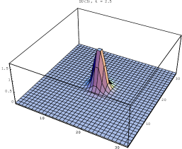
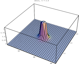
Figure 3: The kinetic energy density on a two dimensional slice through the center of a single texture, which was started with the same initial conditions on the SU(3) and SU(2) codes. This plot comes at the instant of texture collapse, when the field evolution will be least accurate.

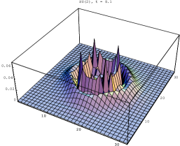
Figure 4: Kinetic energy density on the same slice of the SU(3) and SU(2) simulation, after the texture has collapsed.

5 Results

This code was developed in order to study the effects of cosmic texture, coming from a broken global SU(3) symmetry, upon the early universe. In particular, we would like to use this code to predict the appearance of the cosmic microwave background, if the primordial density fluctuations were seeded by this type of texture. In order to make predictions about the CMBR and density fluctuations, we need to evolve this field forward through the early universe, calculating parts of its energy-momentum tensor as we go: on the large scales of interest, this SU(3) field will interact only gravitationally with the matter and radiation of the early universe. After calculating the necessary parts of the energy-momentum tensor of this field, we can then use this information to predict the power spectrum, nongaussianity, etc. of the CMBR, using previously developed techniques.

In this section we describe the method of uniting this SU(3) evolution code with other codes which evolve the matter and radiation of the early universe, and give some results from these simulations.

5.1 Scaling behavior

In order to use this code to simulate the dynamics of an SU(3) field in the early universe, we need to construct a set of initial conditions. After the initial quench, a physical SU(3) Higgs field would rapidly approach some scaling solution, first in the radiation era and then in the matter era. We do not know, a priori, what the power spectrum of the scaling solution would look like, and so we cannot put in realistic initial conditions. However, if we put in random initial conditions, and evolve the field forward, the simulation itself should also approach scaling behavior. So the first thing we must do is make sure that the SU(3) code does in fact approach a scaling behavior.

In this case, we will look at the scaling behavior of one very important quantity for the growth of gravitational perturbations, namely the source for Newtonian gravity, $\rho+3P\propto T_{00}+T_{ii}$. This acts as the gravitational source term in the scalar density perturbation equations in synchronous gauge (See e.g. [7], [8]). This term alone is sufficient to determine the ‘intrinsic’ perturbations to the CMBR (the synchronous gauge surface terms) and more generally, the matter perturbation power spectrum. A brief calculation shows that for this SU(3) system,

$$T_{00}+T_{ii}=2\left(v_{1}^{2}{\stackrel{{\scriptstyle\mbox{{\huge.}}}}{{\mbox{\boldmath$\psi$}}}}^{2}+v_{2}^{2}{\stackrel{{\scriptstyle\mbox{{\huge.}}}}{{\mbox{\boldmath$\chi$}}}}^{2}\right)\ .$$ (37)

By scaling, we mean the scaling of the power spectrum of this quantity,

$$\left\langle|\phi_{k}(\tau)|^{2}\right\rangle\ ,\qquad\mbox{where\ }\phi_{k}={1\over(2\pi)^{3}V}\int\phi(x,t)e^{-ik\cdot x}{\,\rm d}^{3}x$$ (38)

is the fourier transform of $\phi$. If the simulation is purely in the radiation or matter era, there are no length scales in the system (save the unphysical box size and grid size), so this power spectrum should reflect the scale free nature of the problem. Thus, in the radiation era, we require

$$\left\langle|\phi_{k}(\tau)|^{2}\right\rangle={f(k\tau)\over\tau}$$ (39)

for some function $f(k\tau)$. (The extra factor of $\tau$ is necessary to balance the units; $\phi(x)\sim{\stackrel{{\scriptstyle\mbox{{\huge.}}}}{{\mbox{\boldmath$\psi$}}}}^{2}$ has units of $\tau^{-2}$, and there is a factor of $\tau^{3}$ coming from the expansion of the universe).

Numerically, we take the average in (39) by averaging over the power spectra $\phi_{k}^{2}$ gotten from an ensemble of runs. To test the scaling, behavior we did an ensemble of six runs on $96^{3}$ grids in the radiation era, starting from random initial conditions evenly distributed over SU(3). As can be seen from figure 5, the power spectra in a very wide range of wavenumbers $k$ rapidly approach a scaling solution, and remain on it after $\tau\simeq 6$ grid units.

Figure 5: The power spectrum of $\phi$ approaches scaling in the radiation era. This is a plot of $\tau\left\langle|\phi_{k}(\tau)|^{2}\right\rangle$ vs. $k\tau$, each scaled to remove the box size. Each trace in shows the time evolution of a different fourier mode; each starts at zero because the simulation is started with the fields static, so $\phi(x,0)\sim\dot{\psi}^{2}=0$. Each point on each trace was taken at a time $\tau$ one grid unit later than the preceding point; thus each trace starts at $\tau=0$, has its first joint at $\tau=1$, and so on. (Since the grid is 96 points on a side, the fourier wavenumbers run from k = (1–48)$\cdot{2\pi\over L}$. Thus the range of $k$ shown covers almost all the wavelengths present in the simulation). Each of these fourier modes represents an average of the power spectra from six separate runs. In each run, the power spectrum for a given $|k|$ is an average of power spectra in three perpendicular directions. Thus each point here is an average of eighteen independent quantities.

Since scaling in this power spectrum of $\phi$ begins at $\tau\sim 6$, we can find the scaling function $f(k\tau)$ by averaging the values of $\tau\left\langle|\phi_{k}(\tau)|^{2}\right\rangle$, for all $k$, for times greater than six grid units (and less than half the box size, $\tau<48$ in this case. For times later than this, the box size introduces an unphysical time scale into the problem.) The result of this averaging is shown in 6, which was constructed by summing all the values of $\tau\left\langle|\phi_{k}(\tau)|^{2}\right\rangle$ into bins in $k\tau$.

Figure 6: The averaged scaling function $f(k\tau)$ for SU(3) in the radiation epoch. This is a plot of $f(k\tau)$ vs $k\tau$, and was constructed by averaging all values of $\tau\left\langle|\phi_{k}(\tau)|^{2}\right\rangle$ into bins in $k\tau$. The average runs over all values of $k$, for $\tau$ in a region where the power spectrum is scaling, $6<\tau<40$. The vertical error bars come from assuming that $\phi_{k}(\tau),\phi_{k^{\prime}}(\tau^{\prime})$ will be independent from one another if $k\neq k^{\prime}$. Fourier components with the same wavenumber, at different times, are not assumed to be independent. The horizontal error bars are just the bin sizes.

And with this scaling function, $f(k\tau)$, constructed, we are finally in a position to begin comparing the behavior of SU(3) textures in the early universe with their SU(2) counterparts. A similar set of six runs, on $96^{3}$ grids, in the radiation era, was done using the SU(2) code. Using the same analysis, we constructed a scaling function $f_{{}_{SU(2)}}(k\tau)$. The two functions are shown together in figure 7. The resemblance is striking: up to a multiplicative constant, the two functions are identical to within one another’s error bars. The multiplicative constant is immaterial; it would be removed by normalizing both CMBR predictions to COBE, for example. Thus, at least as far as one can tell from looking at power spectra in the radiation era, SU(3) based textures have almost exactly the same effect upon the early universe as SU(2) based textures do.

Figure 7: A comparison of the scaling functions $f_{{}_{SU(2)}}(k\tau)$ and $f_{{}_{SU(3)}}(k\tau)$. This is a plot of $\log_{10}f$ vs. $\log_{10}k\tau$ for both scaling functions; the SU(2) scaling function is the upper one. Both of these scaling functions were created by averaging power spectra from six radiation era runs on $96^{3}$ boxes.

5.2 CMBR predictions

Finally, we used this code to provide the calculate the appearance of the cosmic microwave background, in a universe where the large scale structure was seeded by SU(3) textures. In the simulations, we start out the field with random initial conditions, and let the field evolve forward in the radiation era long enough for scaling behaviour to set in. We then let the universe transfer from radiation to matter dominated epochs, and continue forward in the matter epoch until the time of last scattering. During this simulation, we used the energy-momentum tensor from the SU(3) field as a gravitational source for the density and velocity fluctuations, using code developed by Crittenden and one of us ([7], [4]).

From the density and velocity perturbations in the primordial gas of one run, in a $256^{3}$ box, we made a set of 48 independant maps of the visible temperature fluctuations on the surface of last scatter. Two such maps, which would appear as $10^{\circ}\times 10^{\circ}$ patches of sky from earth, are shown in figure 8. Superficially, the CMBR anisotropy maps presented here are very similar to previously published textures maps. (See, for example, the pictures in [3].) Note that these maps only represent the intrinsic anisotropies generated on the the surface of last scatter; they do not include the effects from propagating the light from the surface of last scatter to us. This omission has little effect upon the small scale structure of the image, but it does mean that the images have too little power on large angular scales ($l\ \hbox{\lower 4.30554pt\hbox{$\stackrel{{\scriptstyle\mbox{$<$}}}{{\sim}}$}}\ 200$).

Figure 8: Temperature anisotropies on the surface of last scattering. The angular scale of these maps is $10^{\circ}$ on a side, for $\Omega=1$, $\Omega_{B}=0.05$, and $h=.5$. The color scale units are in one standard deviation $\sigma$ for the CMBR anisotropy.

From this assembly of images, one can readily calculate the high end of the CMBR power spectrum, which is shown in figure 9 (along with similar plots from SU(2) textures, cosmic strings, and monopole calculations). Note that these maps don’t contain the necessary large scale information to normalize to COBE, so the normalization of 9 is left arbitrary. We do not expect that the large scale behaviour of the CMBR spectra will be much different between the SU(2) and SU(3) models, when it is calculated: the interesting effects of the nonlinear dynamics show up on small scales. In particular, the positions and shapes of the doppler peaks are correct in this plot. Note that power spectum from the SU(3) textures has a high, second peak, where the SU(2) power spectrum has none, although the position of the first peak is the same. So the SU(3) field dynamics give a bit more power on smaller scales than does SU(2).

Figure 9: The region of the CMBR anisotropy power spectrum dominating on small angular scales for SU(3) textures (filled boxes), SU(2) textures (open boxes), and global monopoles (open triangles). All curves are for $\Omega=1$, $h=.5$. Error bars show the statistical uncertainty (one sigma) in the SU(3) result.

Finally, note that the CMBR maps of 8 contain a handful of extremely high peaks, many more than would be expected in a picture of gaussian fluctuations. These high peaks mark the infall of gas into the gravitational wells created by the energy of the collapse of individual textures: they are a primary source of primordial density fluctuation in this theory. The primary distinguishing features of the textures CMBR maps is an overabundance of large ($\sim$5 sigma) peaks, of which there are O(1) in each map we created. To quantify this, we counted the number of peaks, of a given height, which appear in a given area of sky in the collection of maps that we created. The distribution of peaks for SU(3) and SU(2) textures is shown in 10. Somewhat suprisingly, this measure of the nongaussianity of the maps gives almost indistinguishable results for SU(2) and SU(3) textures. Thus the density of collapsing textures in the universe is almost identical for the two theories.

Figure 10: Differential number of local maxima (and minima) in the CMB anisotropy, of height $\nu\sigma$ (and $-\nu\sigma$) per square degree, where $\sigma$ is the rms. The number density of maxima is shown in solid lines, minima in dotted lines. The filled boxes show the SU(3) texture results, the open boxes the SU(2) results (from ref. [3]).

6 Conclusion

We have developed and used a reliable numerical technique for studying the effects of textures from a broken global SU(3) symmetry upon the early universe. We find that, on the whole, SU(3)-generated textures behave very similarly to textures which come from breaking a global SU(2) symmetry. In particular, the scaling behaviour of the two theories in the radiation era, and the density of nongaussian peaks on the cosmic microwave background, are identical in the two theories to within our numerical errors. We found that the CMBR power spectra of SU(2) and SU(3) textures, are close, but do have a measurable difference in shape: the SU(3) CMBR power spectrum has a bump not present with SU(2) textures. The two textures theories are much closer to one another than they are to qualitatively different theories of large scale structure formation. This suggests that the cosmological predictions of texture theories are rather robust: changing the particular group which is broken to produce the textures has relatively minor cosmological effects. However with the great accuracy one now anticipates in measurements of the CMBR anisotropy power spectrum, even these small differences may be subject to experimental test.

7 Acknowledgements

The computational power necessary for this work was provided through the Pittsburgh Supercomputing Center grant #AST9G3P. We would also like to thank Guy Moore for helpful discussions on computational techniques.

Appendix A The problems from nonuniqueness of $U\rightarrow F$

In section 3, we noted that there were some subtleties in the evolution of the field $F$, the logarithm of the SU(3) field $U$, springing from the non-one-to-one nature of the map between the group and its Lie algebra. In this appendix, we discuss precisely how these subtleties arise in the context of this numerical evolution, and how they are handled. We show that, if treated properly, this ambiguity never presents a problem in the field evolution or interpretation of results.

Recall that the continuum equation for the time derivative of $F$ was of the form:

$$\stackrel{{\scriptstyle\mbox{{\huge.}}}}{{F}}=R\left\{\Omega^{\prime}_{D}+{i\alpha_{{}_{T+}}\over e^{i\alpha_{{}_{T+}}}-1}\Omega^{\prime}_{T+}T_{+}+\ {\rm etc.}\ \right\}R^{-1}\ ,$$

where $\Omega^{\prime}$ was some Lie algebra element, $\Omega^{\prime}_{D}$ is its diagonal part, and the rest is split up in terms of the complexified basis. Here $F$ has been diagonalized into $RF_{D}R^{-1}$, and the $\alpha_{{}_{T+}}$, etc. are simple linear combinations of the components of $F_{D}$. In particular, if we break up $F_{D}$ into the usual generators of the Cartan subalgebra on the main diagonal, $F_{D}=F_{T3}T_{3}+F_{Y}Y$, then the $\alpha\,$s are:

$$\alpha_{{}_{T+}}=F_{T3}\ ,\qquad\alpha_{{}_{U+}}=F_{Y}-{1\over 2}F_{T3}\ ,\qquad\alpha_{{}_{V+}}=F_{Y}+{1\over 2}F_{T3}\ .$$ (40)

For all the generators, $\alpha_{{}_{X-}}=-\alpha_{{}_{X+}}$.

Now, the expression for $\stackrel{{\scriptstyle\mbox{{\huge.}}}}{{F}}$, (30), is written out in terms of functions of the form ${i\alpha\over e^{i\alpha}-1}$ of the six $\alpha\,$s. The behavior of this function needs to be watched carefully, since our time derivatives are expressed in terms of it. It has a removable singularity at the $\alpha=0$, which causes no trouble: the function smoothly approaches $i$ in that region. However, the function has genuine singularities at $\pm 2n\pi$, for all integers $n$ other than zero! Thus if we naïvely evolve the $F$ field forward according to (30) we rapidly get into trouble: the time derivatives go infinite the first time one of the $\alpha\,$s hits $\pm 2\pi.$

And so direct application of (30) only makes sense when we are within a certain neighborhood of the origin in the $F_{T3},F_{Y}$ plane. The situation is illustrated in figure 11: the region of good behavior of all $\alpha\,$s is bounded by a hexagonal wall of singularities of ${i\alpha\over e^{i\alpha}-1}$ in one or more $\alpha$.

Figure 11: The singularities of equation (30), in the plane of the $(T_{3},Y)$ components of $F_{D}$. The dark lines denote places where some $\alpha=2\pi$, so $\alpha(e^{i\alpha}-1)^{-1}$ diverges. The dotted circles denote regions inside which $\alpha(e^{i\alpha}-1)^{-1}<{}$ some chosen bound, for all $\alpha$, for a particular choice of origin.

Now these singularities are not physical, of course; the field equations written in the form of (16), purely in terms of $U$, are not pathological anywhere on the group. The singularities in (30) are just symptoms of the fact that, when $F$ is far enough away from the origin, the coordinate system of the Lie algebra element $F$ is not a very good one for this type of calculation.

The solution to the problem is simply to change origins, whenever we get far away from $F=0$. That is, let us generalize our notation slightly, so that the physical field $U$ is

$$U=e^{iF}{\cal O}\ ,$$ (41)

where ${\cal O}$ is some origin, which we may choose to alter from time to time as we advance the fields forward. The generic effect of adding an origin as in (41) is to change $F$ and its diagonalization:

$$F_{D}\rightarrow F_{D}+\Delta_{D}\ ,\qquad R\rightarrow R^{\prime}\ .$$ (42)

We are permitted to change our origin in any way we please, and so we can always choose the diagonal matrix $\Delta_{D}$ in such a way as to make $F_{D}$ smaller. Provided we monitor the values of $F_{D}$, and change origins whenever it approaches a singular region, we can always avoid any difficulty.

In fact, figure 11 suggests a particularly nice set of origins to use for this purpose. We would like to choose the new origins to be places which are as singular as possible in terms of the old coordinates, so as to keep track of the smallest possible set of origins. As such, the points $A$ and $B$ on figure 11, where two lines of singularities intersect, naturally suggest themselves. (The three points labeled $A$ on figure 11 actually correspond to the same point in SU(3), as do the three points labeled $B$. Every member of SU(3) can be made to correspond to a point in the interior or on the boundary of the hexagon. Within the hexagon, there is a three-fold “reflection” symmetry coming from the ambiguity of how we choose to order the eigenvalues of $F$ within $F_{D}$). In fact, the SU(3) members gotten by exponentiating $A$ and $B$ are just $e^{i\pi/3},\ e^{2i\pi/3}$ times the identity: together with 1, they form the center of SU(3). These points are particularly nice origins because they make changing origin very easy; they commute with everything. In particular, the transformation of the $R$ matrix in (42) becomes trivial, whereas in general it is a painful thing to compute.

So: the evolution algorithm described in section 3 is modified as follows. Each time we diagonalize $F$, we construct the radius² $F_{T3}^{2}+F_{Y}^{2}$ and figure out how far we are from our current origin in figure 11. If we are outside of a certain radius, we declare it time to change origins, and shift the origin of $F$ to the corner of the hexagon nearest to the current position of $F_{D}$. (We must also shift the origin of the previous timestep in the same way, because the algorithm uses the previous timestep directly with this one.) The only thing that need be decided systematically is which cutoff circle to use. From figure 11 we see that the radius must be greater than ${4\pi\over 3}$, so that the three circles centered at $1,A,B$ intersect, and less than $2\pi$, to avoid the nearest singularity. We chose $3\pi\over 2$, which provides a nice region of intersection, but is far enough away from the nearest singularities that the time derivatives never become too big; $(3\pi/2)|(e^{3i\pi/2}-1)^{-1}|\simeq 3.3$ is the largest value obtained by the diverging function in that region. (The smallest value obtained is 1, at the origin). Now, since the entire calculation of $\stackrel{{\scriptstyle\mbox{{\huge.}}}}{{F}}$ will always be within some circular region in which $\stackrel{{\scriptstyle\mbox{{\huge.}}}}{{F}}$ is well behaved, we never encounter any problems.

Everything else proceeds as before. Of course, we must now keep track of which of the three origins associated with each grid point, and make use of the origin as in (41) whenever we construct $U$. Fortunately, the simple form of the three origins chosen means that this does not slow down the program very much.

Appendix B Discretized derivatives of $T_{\mu\nu}$.

In section 4, we describe the constructing the discrete derivatives of the energy-momentum tensor, in order to test how well the numerical algorithm obeys local conservation of energy, $\partial^{\mu}T_{\mu 0}=0.$ When discretized, this becomes

$$\delta_{0}T_{00}-\delta_{i}T_{0i}=\epsilon\ ,$$

where $\epsilon$ is the error we seek to measure. Now, (35) involves a time derivative of the 00 component of $T$. A discrete version of $T_{00}$ lives most naturally upon a grid point on a whole timestep. The momentum densities $T_{0i}$ involve constructs like $\partial_{x}\mbox{\boldmath$\psi$}^{\dagger}\partial_{0}\mbox{\boldmath$\psi$}$, and so most naturally live on the links between grid points, though on whole timesteps. (We place the time derivatives, $\stackrel{{\scriptstyle\mbox{{\huge.}}}}{{\mbox{\boldmath$\psi$}}},\stackrel{{\scriptstyle\mbox{{\huge.}}}}{{\mbox{\boldmath$\chi$}}}$ on whole timesteps since we need to use both $U$ and $L$ to construct these. The $L$ grid lives on half timesteps, while $U$ lives on whole timesteps, so one or the other will have to be averaged to produce a $\stackrel{{\scriptstyle\mbox{{\huge.}}}}{{U}}$ at a single point. Since $L$ lives in an algebra, averages of two $L$ are meaningful, whereas naïve averages of two values of $U$ are not. Thus we chose to construct time derivatives which live on whole timesteps.) Since equation (35) itself involves a time derivative of $T_{00}$ and spatial derivatives of the $T_{0i}$, the discrete version of it may be fairly easily centered on a whole grid point, on a half timestep.

$$\delta_{0}T_{00} = {1\over\Delta_{\tau}}\left(T_{00}^{n+1}-T_{00}^{n}\right)\ ,\qquad\mbox{where}$$ (43)

$$T_{00}^{n} = v_{1}^{2}\left(\stackrel{{\scriptstyle\mbox{{\huge.}}}}{{\mbox{\boldmath$\psi$}^{\dagger}_{n}}}\stackrel{{\scriptstyle\mbox{{\huge.}}}}{{\mbox{\boldmath$\psi$}}}_{n}\right)+{v_{1}^{2}\over 2\Delta_{x}^{2}}\Bigl{(}\left|\mbox{\boldmath$\psi$}^{i+1}_{n}-\mbox{\boldmath$\psi$}^{i}_{n}\right|^{2}+\left|\mbox{\boldmath$\psi$}^{i}_{n}-\mbox{\boldmath$\psi$}^{i-1}_{n}\right|^{2}$$ (44)

$$\qquad\qquad+\mbox{ similar terms in $j$, $k$ directions}\Bigr{)}\ ,$$

with a parallel term for $\chi$. Here the $\stackrel{{\scriptstyle\mbox{{\huge.}}}}{{\mbox{\boldmath$\psi$}}}$ terms are calculated from the $L$ field, using the mean between the two half steps, as in (33). Next we need to construct a discrete version of $\partial_{x}T_{0x}$ which lives on a whole grid point, on a half timestep. Since the $T_{0x}$ live on whole timesteps, on links between lattice sites, this must be constructing by differencing adjacent links, and averaging between two timesteps. In one direction, this gives:

$$\left.\delta_{x}T_{0x}\right|^{n+1/2,i} = {1\over 2\Delta_{x}}\biggl{\{}\left(T^{n,i+1/2}_{0x}-T^{n,i-1/2}_{0x}\right)+$$ (45)

$$\qquad\qquad\left(T^{n+1,i+1/2}_{0x}-T^{n+1,i-1/2}_{0x}\right)\biggr{\}}\ ,\qquad\mbox{where}\quad$$

$$T^{n,i+1/2}_{0x} = {1\over 2\Delta_{x}}v_{1}^{2}\,{\rm Re}\left\{\left(\stackrel{{\scriptstyle\mbox{{\huge.}}}}{{\mbox{\boldmath$\psi$}^{i}_{n}}}+\stackrel{{\scriptstyle\mbox{{\huge.}}}}{{\mbox{\boldmath$\psi$}^{i+1}_{n}}}\right)^{\dagger}\left(\mbox{\boldmath$\psi$}^{i+1}_{n}-\mbox{\boldmath$\psi$}^{i}_{n}\right)\right\}\ ,$$ (46)

with, again, a similar term for $\chi$.

These are the explicit forms used for the tests of local energy conservation used in section 4. They are shown here in detail because there several possible ways of constructing these discrete $T_{\mu\nu}$ components and their discrete derivatives, and most of them do not work.

References

- [1] N. Turok, Phys. Rev. Lett. 63 2625 (1989)
- [2] J.A. Bryan, S.M. Carroll and T. Pyne, hep/ph 9312254, Phys. Rev. D 50, 2806 (1994).
- [3] U. Pen, D. Spergel, N. Turok, Phys. Rev. D 49 692 (1994)
- [4] N. Turok, Ap. J. Lett. 473, L5 (1996).
- [5] A. Sornberger, S.M. Carroll and T. Pyne, hep/ph 9701351.
- [6] M. Joyce and N. Turok, Nuc. Phys. B 416, 389 (1994)
- [7] R.G. Crittenden and N. Turok, Phys. Rev. Lett 75 2642 (1995).
- [8] R. Durrer, A. Gangui and M. Sakellariadou, Phys. Rev. Lett. 76, 579 (1996).
- [9] T. Cheng and L. Li, Gauge theory of elementary particle physics, Oxford University Press, 1992.