Abstract

A new perturbative scheme is proposed for the evaluation of the free energy density of field theories at finite temperature. The screened loop expansion takes into account exactly the phenomenon of screening in thermal propagators. The approach is tested in the $N$-component scalar field theory at 2-loop level and also at 3-loop in the large $N$ limit. The perturbative series generated by the screened loop expansion shows much better numerical convergence than previous expansions generated in powers of the quartic coupling.

PACS: 11.10.Wx, 12.38.Mh
Keywords: QCD, scalar field theory, free energy density, Debye screening, loop expansion, gap equation, high-T expansion

1 Introduction

The weak coupling expansion of the QCD free energy density does show very bad convergence properties. The coefficients of the usual perturbative series are of alternating sign and of increasing magnitude [1]-[6] Only in the TeV temperature range can one find a satisfactory numerical convergence rate [7]. This is in great contrast to numerical calculations of this quantity (or of its derivative, the internal energy) in Monte Carlo simulations. These calculations indicate that deviations from the high temperature ideal gas limit are within 15% already for temperatures about twice the critical temperature [8].

On the other hand it has been observed already quite some time ago that the formula for the free energy density of a massive ideal gas does give a quite satisfactory description of the numerical simulations [9]. Such a description leads to results about 10% below the Monte Carlo data. Although such an approach clearly has to be refined in order to take care of the correct number of degrees of freedom and the modifications due to interactions it indicates that a representation of a perturbative expansion in terms of massive degrees of freedom might be a good starting point.

This observation leads us to conjecture that the apparent poor convergence of the perturbatively calculated free energy density might be improved if the series is reorganised into a loop expansion evaluated with screened propagators; i.e. instead of expanding around the massless ideal gas limit, we intend to perform the loop expansion starting from a massive ideal gas.

There are several screening scales in QCD, which makes the practical application of this conjecture more complicated, than it looks like at first sight. In the scalar theory, on the other hand, the only relevant mass is the Debye screening mass. For this reason we will discuss here only the calculation of the free energy density of the $N$ component scalar $\Phi^{4}$-theory. The problem of poor numerical convergence shows up equally well already here [10, 11, 12]. One thus can test to what extent the above mentioned reorganisation of the perturbation series improves the convergence.

We shall calculate and analyze first the two-loop correction to the massive ideal gas formula. With respect to their screening mass dependence our formulae are exact. The ultra-violet finiteness of our calculation is ensured without the need to fix the screening mass inherently. As an external information we shall use for the screening mass the root of the corresponding 1-loop gap equation [14, 15, 16]. For large $N$ it also is possible to estimate the 3-loop correction of the free energy density. Finally, we shall compare the results obtained with this screened perturbative expansion with those obtained from the conventional resummation scheme [5, 10, 11, 12] as well as from an effective theory approach [13].

2 Loop Expansion with Debye Screened Propagators

We consider an $O(N)$ symmetric scalar field theory with the following Lagrangian:

$$L=L_{0}+L_{int},$$

$$L_{0}={1\over 2}({(\partial\phi_{i})}^{2}+m^{2}\phi^{2}_{i}),$$

$$L_{int}=-{1\over 2}m^{2}\phi_{i}^{2}+{g^{2}\over 24N}{(\phi_{i}^{2})}^{2}+{g^{2}\over 24N}(Z_{2}-1){(\phi_{i}^{2})}^{2}.$$ (1)

Following ref. [10, 11] we have introduced and substracted a mass term with $m\sim{\cal O}(g)$ in order to reorganize the perturbative expansion. The coupling constant renormalisation factor is given by [17]

$$Z_{2}=1+{3g^{2}\over{(4\pi)}^{2}}{N+8\over 18\epsilon}+{\cal O}(g^{4}),$$ (2)

and we have left out the field renormalisation factor $Z_{1}$, which is unity up to ${\cal O}(g^{4})$.

All Feynman diagrams contributing to the free-energy density up to 3-loops can be found in [5]. The contribution of these diagrams are:

$$-F^{(a)} = -{1\over 2}NJ(m),$$

$$-F^{(b)} = -{1\over 8}g^{2}\tilde{N}I(m)^{2},$$

$$-F^{(c)} = {1\over 2}m^{2}NI(m),$$

$$-F^{(d)} = -g^{4}\tilde{N}{N+8\over 48N}{1\over{(4\pi)}^{2}\epsilon}I(m)^{2},$$

$$-F^{(e)} = {1\over 4}m^{4}NI^{\prime}(m),$$

$$-F^{(f)} = -{g^{2}m^{2}\over 4}\tilde{N}I(m)I^{\prime}(m),$$

$$-F^{(g)} = {g^{4}\over 16N}\tilde{N}^{2}I(m)^{2}I^{\prime}(m),$$

$$-F^{(h)} = {g^{4}\over 48N}\tilde{N}I_{ball}(m),$$

$$F=F^{(a)}+F^{(b)}+F^{(c)} + F^{(d)}+F^{(e)}+F^{(f)}+F^{(g)}+F^{(h)}.$$ (3)

Here we have used the same labeling of the diagrams as in [5]. Furthermore, we use the abbreviation $\tilde{N}=(N+2)/3$ and have introduced the following notation for the relevant integrals:

$$J(m) = \int_{P}\log(P^{2}+m^{2}),$$ (4)

$$I(m) = \int_{P}{1\over P^{2}+m^{2}},$$ (5)

$$I^{\prime}(m) = \int_{P}{1\over{(P^{2}+m^{2})}^{2}},$$ (6)

$$I_{ball}={\displaystyle\int_{PQKR}{1\over{(P^{2}+m^{2})(Q^{2}+m^{2})(K^{2}+m^{2})(R^{2}+m^{2})}}}\delta(P+Q+K+R).\\$$

Here we are using dimensional regularisation at finite temperature. The symbol $\int_{P}$ therefore is understood to represent $T\sum_{n=-\infty}^{\infty}\int{d^{3-2\epsilon}p\over{(2\pi)}^{3-2\epsilon}}$. We note that all relevant sum-integrals appearing in Eqs.(3-7) are UV-singular and do depend on the renormalisation scale $\mu$. We shall argue below that a consistent expansion is obtained by simply dropping these terms at each order in the loop expansion.

At two loop level only the diagrams (a-c) contribute. As will be discussed below we have, at present, difficulties to extend our analysis at finite $N$ to 3-loops because we cannot handle the finite terms in the “basketball” diagram (h) for nonzero values of the screening mass. We have, however, also listed the 3-loop diagrams here, since the contribution from diagram (h) is suppressed in the large $N$ limit. We are therefore also going to analyze the behaviour of our screened perturbative expansion in this limit by including the 3-loop contributions (d-g).

We have explored two possibilities to evaluate the 1-loop integrals $J(m)$, $I(m)$ and $I^{\prime}(m)$. The first consists of performing the Matsubara sum using the contour trick, subtract the $T=0$ piece, and then evaluate the remaining three-dimensional integral numerically. For $J(m)$ we obtain

$$J(m)={\mu}^{2\epsilon}\int{d^{3-2\epsilon}p\over{(2\pi)}^{3-2\epsilon}}\sqrt{p^{2}+m^{2}}+2{\mu}^{2\epsilon}\int{d^{3-2\epsilon}p\over{(2\pi)}^{3-2\epsilon}}\log(1-e^{-{\sqrt{p^{2}+m^{2}}\over T}}).$$ (7)

The other two integrals, $I(m)$ and $I^{\prime}(m)$, can be obtained from this by simple differentiation with respect to $m^{2}$. The other possibility to evaluate these sum-integrals is to use directly the high-T expansion of the integrals $J(m)$, $I(m)$ and $I^{\prime}(m)$ which can be found in [18].

The leading order 1-loop result is given by diagram (a), i.e. $F^{(a)}$. It represents the contribution of a massive ideal gas. However, on its own this contribution is not complete. It contains UV-divergent and scale dependent contributions [18]. The divergent piece is proportional to $m^{4}/\epsilon$. Since the screening mass is linearly depending on $T$ this divergent term cannot be canceled by the subtraction of appropriate zero temperature contributions. Higher loop contributions should take care of the cancellation of temperature dependent singularities. As the screening mass is ${\cal O}(gT)$ we expect that two and three loop contributions are needed to cancel the leading poles in $\epsilon$. In fact, it is easy to check, that this is the case. Collecting all poles in $\epsilon$ with residua proportional to $m^{4},g^{2}T^{2}m^{2},g^{4}T^{4}$ coming from diagrams up to 3-loop, we find that the singular terms cancel irrespective of the actual value of $m^{2}$.

This observation forms the basis for our conjecture: The ultra-violet, temperature dependent singularities appearing in a given order of the screened loop expansion will be canceled by appropriate contributions from higher order loops. At any given order in the expansion these singular contributions thus can be dropped.

At two loop order there appear also singularities with poles in $\epsilon^{2}$ as well as poles with higher powers of $m^{2}$. In order to check explicitly the cancellation of these singularities we would need to know the complete 4-loop contribution to the free energy density. This is not known. We thus invoke the above conjecture to eliminate these singular terms from the expansion.

Another question which has to be investigated is the dependence on the renormalisation scale. In the conventional perturbative approach the scale dependence appears first at 3-loop level. The scale dependent contributions appearing in the 1-loop and 2-loop results (see the explicit expressions of $J(m)$ and $I(m)$ in [18]) usually are canceled by corresponding zero temperature contributions. In the screened perturbative approach this again cannot be achieved because the scale dependent terms are proportional to the temperature, i.e. the screening mass. However, these additional scale dependent terms, proportional to the screening mass, are canceled by higher loop contributions in analogy to the singular terms discussed above. Furthermore, the screening mass independent scale dependence of the 3-loop contribution is exactly canceled when one takes into account the scale dependence of the coupling constant in the 2-loop diagrams. Up to ${\cal O}(g^{4})$ the free energy is thus scale independent [13]. We therefore omit terms proportional to $\ln({\bar{\mu}}^{2}/T^{2})$ in the lower loop expressions, too.

Finally, we have to specify the screening mass. Since $m^{2}$ has remained undetermined we have specified it as the exact root of the gap equation relevant for the chosen order of the loop expansion, i.e. we use the 1-loop gap equation without expanding $I(m)$ in its argument:

$$m^{2}={g^{2}\tilde{N}\over 2N}(I(m)+{m^{2}\over 16\pi^{2}}({1\over\epsilon}+\ln{{\bar{\mu}}^{2}\over T^{2}})).$$ (8)

Below we shall use roots of Eq. (8) for the analysis of the free energy density. The screening mass obtained this way agrees well with the 1-loop value for $g\raise 1.29167pt\hbox{$<$\kern-7.5pt\raise-4.73611pt\hbox{$\sim$}}1$ while it is only half as large as the 1-loop value for $g\sim 10$. We also note that as a consequence of using the root of the gap equation for $m^{2}$, no term proportional to $g^{2}m$ will appear in the free energy density. Such a term is seen to exist in $F^{(b)}$ when we use the high-T series for $I(m)$. However, this contribution is canceled by part of $F^{(c)}$, when exploiting (8). The entire cubic dependence on $g^{3}$, which partly is responsible for the poor convergence of the conventional perturbative expansion, is now hidden in a term proportional to $m^{3}$ which contributes to $J(m)$.

3 Numerical Results

We have evaluated the free energy density using Eq. (3) without making any assumption about the magnitude of $m$, i.e. we have calculated $F$ ”exactly” in $m$. For finite $N$ we can do this so far only at 2-loop level. At 3-loop one would have to calculate the finite part of $I_{ball}(m)$ for arbitrary values of $m$. Since we are not assuming that $m$ is small we did use the integral representations for $J(m)$, $I(m)$ and $I^{\prime}(m)$ in our numerical calculations. However, we also checked the alternative approach based on the high-T expansion and found that this series does converge rapidly. For the integrals listed above it is sufficient to take the first six terms of high-T expansion for $g\in[0,12]$.

In Fig 1. we show the 1-loop and 2-loop results for the free energy density as function of the self-coupling $g$ and for $N=1$. The screening mass has been computed from Eq. (8). Also shown there are the results obtained with the conventional perturbative expansion up to ${\cal O}(g^{2})$ and ${\cal O}(g^{3})$ in the scalar self-coupling. The Figure clearly shows that the difference between 1-loop and 2-loop results of the screened perturbative expansion is small and essentially stays constant over the entire range of couplings. In the conventional perturbative approach on the other hand different orders in the expansion differ largely from each other.

For large $N$ the contribution of the basketball diagram is suppressed by $1/N$ relative to other diagrams. In this limit we thus can consider also the 3-loop result. In the large-$N$ limit the 1-loop gap equation (8) becomes exact. Its derivation as a Schwinger-Dyson equation has been given in [14]. The setting sun diagram with exact vertex becomes negligible in the large N limit, while the divergent and scale dependent part of the tadpole contribution is canceled by the renormalisation of the scalar self-coupling.

For our numerical investigation of the large-N limit we have chosen $N=10$. The 1-loop, 2-loop and 3-loop results for the free energy density obtained from the screened perturbative expansion are shown in Fig. 2. The screening mass has been determined from Eq. (8). For comparison we also show the conventional ${\cal O}(g^{4})$ result of [5]. Lower orders in this approach do show alternating behaviour similar to that shown in Fig. 1 for the case $N=1$. We note that like in the $N=1$ case the higher loop corrections lead to smaller deviations from the massless ideal gas than the leading 1-loop result. We also find that for $g<12$ the difference between the 3-loop result and the massless ideal gas limit is only $10\%$.

4 Conclusions

We have formulated a perturbative scheme for the $N$-component scalar field theory which includes a temperature dependent screening mass in the scalar propagator. We conjecture that a systematic loop expansion is obtained when singular terms and scale dependent terms proportional to the screening mass are dropped order by order in the perturbative expansion. This expansion coincides to all orders with the conventional approach, if the screening mass is treated perturbatively. Within the screened perturbative approach we can handle the effect of a screening mass exactly.

The analysis of the $N=1$ scalar field theory and its large-$N$ limit to 2-loop and 3-loop, respectively, shows that within this approach the convergence of the perturbative series is drastically improved over the conventional approach. It is also evident that taking into account higher orders in the massive loop expansion systematically brings the free energy density closer to the massless ideal gas limit. It certainly would be interesting to test these results against non-perturbative lattice calculations.

We hope that the nice properties seen here for the scalar theory remain valid also in the case of QCD where more mass scales will become relevant.

Acknowledgement P.P. thanks  J. Polónyi and Z. Fodor for useful discussions.

Figure Caption

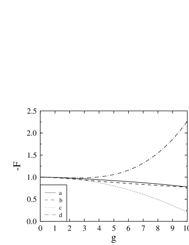
Figure 1: Shown is the free-energy density of the N=1 scalar field theory as a function of the scalar self-coupling g in the units of the free energy density of a massless ideal gas ($\pi^{2}T^{4}\over 90$). The curves represent 2-loop (a) and 1-loop (b) results of the screened loop expansion as well as the ${\cal O}(g^{2})$ (c) and ${\cal O}(g^{3})$ (d) results of the conventional perturbative expansion.

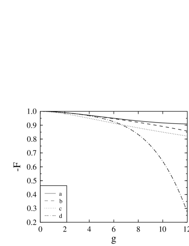
Figure 2: The free energy density of the scalar field theory in the large-$N$ limit as a function of the scalar self-coupling $g$ in units of the free energy density of a massless ideal gas. Shown are results for $N=10$ (see text). The curves represent 3-loop (a) 2-loop (b) and 1-loop (c) results of the screened loop expansion as well as the ${\cal O}(g^{4})$ (d) results of the conventional perturbative expansion.

References

- [1] E. Shuryak, JETP, 47 (1978) 212
- [2] J. Kapusta, Nucl. Phys. B148, (1979) 461
- [3] K. Kalashnikov and J. Klimov, Sov. J. Nucl. Phys. 33 (1981) 647
- [4] A. Toimela, Phys. Lett. 124B (1983) 407
- [5] P. Arnold and C. Zhai, Phys. Rev. D50 (1994) 7603 and Phys. Rev. D51 (1995) 1906
- [6] B. Kastening and C. Zhai, Phys. Rev. D52 (1995) 7232
- [7] A. Nieto, Perturbative QCD at High Temperature OHSTPY-HEP-T-96-019, hep-ph/9612291
-
[8]
F. Karsch, in ”QCD, 20 Years Later”, eds P.M. Zerwas
and
H.A. Kastrup, World Scientific 1993, pp 717-748
G. Boyd, J. Engels, F. Karsch, E. Laermann, C. Legeland, M. Lütgemeier, B. Petersson, Nucl.Phys. B469 (1996) 419 - [9] F. Karsch, Nucl. Phys. B9 [Proc. Suppl.] (1989) 357
- [10] J. Frenkel, A. Saa, and J. Taylor, Phys. Rev. D46 (1992) 3670
- [11] R. Parwani, Phys. Rev. D45 (1992) 4965
- [12] R. Parwani and H. Singh, Phys. Rev. D51 (1995) 4518
- [13] E. Braaten and A. Nieto, Phys. Rev. D51 (1995) 6990
- [14] L. Dolan and R. Jackiw, Phys. Rev. D9 (1974) 3320
- [15] W. Buchmüller, Z. Fodor, T. Helbig and D. Walliser, Ann. Phys. 234 (1994) 260
- [16] J.R. Espinosa, M. Quirós and F. Zwirner, Phys. Lett. 314 (1993) 206
-
[17]
D.J. Amit,
Field Theory, Renormalisation Group and
Critical Phenomena, chapter 7, p.173 (1978, McGaw-Hill Inc). - [18] P. Arnold and R. Espinosa, Phys. Rev. D47 (1993) 3546