hep-ph/9702354 CERN-TH/97-25

NTZ 97/6

Scale dependence of the chiral-odd twist-3

distributions $h_{L}(x)$ and $e(x)$

A.V. Belitsky

Bogoliubov Laboratory of Theoretical Physics

Joint Institute for Nuclear Research

141980, Dubna, Russia

D. Müller

Theory Division, CERN,

CH-1211 Geneva 23, Switzerland

Abstract

We evaluate the complete leading-order evolution kernels for the chiral-odd twist-3 distributions $e(x)$ and $\widetilde{h}_{L}(x)$ of the nucleon. We establish the connection between the evolution equations in light-cone position and light-cone fraction representations, which makes a correspondence between the non-local string operator product expansion and the QCD-inspired parton model. The compact expression obtained for the local anomalous dimension matrix coincides with previous calculations. In the multicolour QCD as well as in the large-$x$ limit the twist-3 distributions obey simple DGLAP equations. Combining these two limits, we propose improved DGLAP equations and compare them numerically with the solutions of the exact evolution equations.

CERN-TH/97-25
February 1997

1 Introduction

The factorization theorems [1] provide us with powerful tools to study the processes with large momentum transfers. They give us the possibility to separate the contributions responsible for physics of large and small distances. The former are parametrized by the hadron’s parton distribution functions, or by parton correlators in general, which are uncalculable at the moment from the first principles of the theory, while the second ones — hard-scattering subprocesses — can be dealt perturbatively. The parton distributions are defined in QCD by the target matrix elements of the light-cone correlators of field operators [2]. This representation allows for the estimation of these quantities by the non-perturbative methods presently available, which are close to the fundamental QCD Lagrangian [3].

The increasing accuracy of the experimental measurements requires the unravelling of the twist-3 effects in the hard processes, which manifest the quantum mechanical interference of partons in the interacting hadrons. The most important advantage of the twist-3 structure functions is that, while being important for understanding the long-range quark–gluon dynamics, they contribute at leading order in $1/Q$ ($Q$ being the momentum of the probe) to certain asymmetries [4, 5] and therefore may be directly extracted from experiments [6]. To confront the theory with high-precision data, the knowledge of the scale dependence of the measurable quantities is needed. The $Q^{2}$ evolution of the parton distributions [7, 8] can be predicted by exploiting the powerful methods of renormalization group (RG) and QCD perturbation theory. The evolution equation of the twist-3 polarized chiral-even nucleon structure function $g_{2}(x)$ was extensively discussed in the literature [9]–[13] as well as its solution in the multicolour QCD and asymptotical values of orbital momentum $n\to\infty$ ($x\to 1$ region) [14].

In this paper we address the study of the evolution of other twist-3 structure functions of the nucleon: chiral-odd distributions $e(x)$ and $h_{L}(x)$ [5], which open a new window to explore the nucleon content. The present study was induced by several reasons and pursues various goals. First, while the anomalous dimensions of the local operators corresponding to the moments of the chiral-odd distributions were computed for the real QCD case [15], the kernels of the evolution equations were derived only in the multicolour limit [16]. From the point of view of experimental measurements, the knowledge of the evolution of the whole $x$-dependent distribution is welcome. However, exact equations that takes into account the ${\cal O}(1/N_{c}^{2})$ effects are lost, although we may expect sizeable $1/N_{c}^{2}$ effects for the small-$x$ behaviour of the distribution functions, provided the non-leading terms in $N_{c}$ yield the rightmost singularity in the complex $n$-plane of the angular momentum with respect to the leading-order result. Second, up to now the relation between different formulations of the evolution equations in the light-cone fraction [9, 10] and light-cone position [11, 17] representations was obscure. So, the aim of the present paper is two fold: to fill the gap in our knowledge of the exact (taking into account of the $1/N_{c}^{2}$ effects) higher-twist evolution equations for chiral-odd distributions and to provide the relation between different calculational approaches. We attempt here to clarify these issues.

The outline of the paper is the following. We start with the construction of the basis of the twist-3 chiral-odd polarized and unpolarized correlation functions, mixed under the renormalization group evolution, and find the equations that govern their scale dependence in the momentum fraction as well as in the light-cone position representations in Section 2. In Section 3 we present the Fourier transformation of the evolution kernels, which simplifies the transition from one representation to another. Section 4 is devoted to the construction of the generalized DGLAP equation in mixed representation for the twist-3 distributions, which is the most useful for solving the RG equations in the large-$N_{c}$ limit as well as for asymptotical values of the orbital momentum $n$. The corresponding analytical solution, as well as a numerical study of exact equations is performed in Section 5. The final Section contains a discussion and concluding remarks.

To make the discussion complete and more transparent, we include several appendices. In Appendix A we present definitions and some properties of the $\Theta$-functions that appeared in the formulation of the evolution equations in the momentum space. In Appendix B the evolution equations for the redundant basis of operators are found in the Abelian gauge theory. This shows the self-consistency of the whole approach. The anomalous-dimension matrix of local twist-3 operators obtained from the evolution equations we have derived in the main text are written in Appendix C. It coincides with results known in the literature [15].

2 Evolution of chiral-odd twist-3 correlation functions

As we mentioned in the Introduction, the parton distribution functions in QCD are defined by the Fourier transforms along the null-plane of the forward matrix element of the parton field operators product separated by an interval $\lambda$ on the light cone:

$${\cal F}(\lambda)\equiv{\cal F}(\lambda,0)=\phi^{*}(0)\phi(\lambda n),$$ (1)

where $\phi$ denotes a quark $\psi$ or a gluon field $B_{\mu}$. We suppress the dependence on the renormalization scale $\mu_{R}$, necessary to make this equation well defined in field theory. Throughout the paper we use the ghost-free $B_{+}\equiv B_{\mu}n^{\mu}=0$ gauge. Here $n$ is a light-cone vector $n^{2}=0$ normalized with respect to the four-vector $P=p+\frac{1}{2}M_{h}^{2}n$ of the parent hadron $h$ of mass $M_{h}$, i.e. $nP=1$, and $p$ is a null vector along the opposite tangent to the light cone such that $p^{2}=0$, $np=0$. In any covariant gauge a path-ordered link factor should be inserted between the $\phi$-fields so as to maintain the gauge invariance of the physical quantities. The Fourier transformations from the coordinate to the momentum space and vice versa are given by

$$F(x)=\int\frac{d\lambda}{2\pi}e^{i\lambda x}\langle h|{\cal F}(\lambda)|h\rangle,\hskip 14.22636pt\langle h|{\cal F}(\lambda)|h\rangle=\int dxe^{-i\lambda x}F(x).$$ (2)

Both of these representations display the complementary aspects of the factorization. The light-cone position representation is suitable to make contact with the operator product expansion (OPE) approach, while the light-cone fraction representation is appropriate for establishing the language of the parton model. Throughout the paper we will use the light-cone position and the light-cone fraction representations in parallel.

The multiparton distributions corresponding to the interference of higher Fock components in the hadron wave functions that emerge at the twist-3 level are the generalizations of (1) to 3-parton fields

$${\cal F}(\lambda,\mu)\equiv{\cal F}(\lambda,0,\mu)=\phi^{*}(\mu n)\phi(0)\phi(\lambda n).$$ (3)

We do not display the quantum numbers of the field operators since they are not of relevance at the moment. The direct and inverse Fourier transforms are

$$F(x,x^{\prime})=\int\frac{d\lambda}{2\pi}\frac{d\mu}{2\pi}e^{i\lambda x-i\mu x^{\prime}}\langle h|{\cal F}(\lambda,\mu)|h\rangle,\hskip 14.22636pt\langle h|{\cal F}(\lambda,\mu)|h\rangle=\int dxdx^{\prime}e^{-i\lambda x+i\mu x^{\prime}}F(x,x^{\prime}).$$ (4)

The variables $x$ and $x^{\prime}$ are the momentum fractions of incoming $\phi$ and outgoing $\phi^{*}$ partons, respectively. The restrictions on their physically allowed values come from the support properties of the multiparton distribution functions discussed at length in Ref. [19], namely $F(x,x^{\prime})$ vanishes unless $0\leq x\leq 1$, $0\leq x^{\prime}\leq 1$.

Beyond the leading-twist level the intuitive parton-like picture is not so immediate, as one usually starts with an overcomplete set of correlation functions. However, the point is that the equations of motion for field operators imply several relations between correlators, and the problem of construction of the simpler operator basis is reduced to an appropriate exploitation of these equalities. The guiding line to disentangle the twist structure is clearly seen in the light-cone formalism of Kogut and Soper [18]. Consider, for instance, the correlators containing two quarks $\bar{\psi}\psi$. Then decomposing the Dirac field into “good” and “bad” components with Hermitian projection operators ${\cal P}_{\pm}=\frac{1}{2}\gamma_{\mp}\gamma_{\pm}$: $\psi_{\pm}={\cal P}_{\pm}\psi$, we have three possible combinations $\psi^{\dagger}_{+}\psi_{+}$, $\psi^{\dagger}_{+}\psi_{-}\pm\psi^{\dagger}_{-}\psi_{+}$, and $\psi^{\dagger}_{-}\psi_{-}$, which are of twist 2, 3 and 4, respectively. The origin of this counting lies in the dynamical dependence of the “bad” components of the Dirac fermions

$$\psi_{-}=-\frac{i}{2}\partial^{-1}_{+}\left(i\not\!\!D_{\perp}+m\right)\gamma_{+}\psi_{+}.$$ (5)

These components depend on the underlying QCD dynamics, i.e. they implicitly involve extra partons and thus correspond to the generalized off-shell partons, which carry the transverse momentum. For this reason we come back to the on-shell massless collinear partons of the naive parton model, but supplemented with multiparton correlations through the constraint (5). The operators constructed from the “good” components only were named quasi-partonic [10]. The advantage of handling them is that they endow the theory with a parton-like interpretation for higher twists.

At the twist-3 level the nucleon has two chiral-odd distributions $e$ and $h_{L}$ , which can be measured in the polarized Drell–Yan and semi–inclusive DIS processes. Under QCD evolution, they couple to complicated quark–gluon operators and correlation functions, depending on the quark mass and intrinsic transverse momentum. We will treat below the unpolarized and polarized cases separately.

2.1 Unpolarized distributions

In the unpolarized case we define the following redundant basis chiral-odd twist-3 correlation functions:

$$e(x)=\frac{x}{2}\int\frac{d\lambda}{2\pi}e^{i\lambda x}\langle h|\bar{\psi}(0)\psi(\lambda n)|h\rangle,$$ (6)

$$M(x)=\frac{1}{2}\int\frac{d\lambda}{2\pi}e^{i\lambda x}\langle h|\bar{\psi}(0)m\gamma_{+}\psi(\lambda n)|h\rangle,$$ (7)

$$D_{1}(x,x^{\prime})=\frac{1}{2}\int\frac{d\lambda}{2\pi}\frac{d\mu}{2\pi}e^{i\lambda x-i\mu x^{\prime}}\langle h|\bar{\psi}(\mu n){\rm g}\gamma_{+}\!\not\!\!B^{\perp}(0)\psi(\lambda n)|h\rangle,$$ (8)

$$D_{2}(x^{\prime},x)=\frac{1}{2}\int\frac{d\lambda}{2\pi}\frac{d\mu}{2\pi}e^{i\mu x^{\prime}-i\lambda x}\langle h|\bar{\psi}(\lambda n){\rm g}\!\not\!\!B^{\perp}(0)\gamma_{+}\psi(\mu n)|h\rangle.$$ (9)

The functions $D_{1}$ and $D_{2}$ are related by complex conjugation $\left[D_{1}(x,x^{\prime})\right]^{*}=D_{2}(x^{\prime},x)$. The quantities determined by these equations form a closed set under renormalization; however, they are not independent, since there is a relation between them due to the equation of motion for the Heisenberg fermion field operator:

$$e(x)-M(x)-\int dx^{\prime}D(x,x^{\prime})=0,$$ (10)

where we have introduced the convention

$$D(x,x^{\prime})=\frac{1}{2}\left[D_{1}(x,x^{\prime})+D_{2}(x^{\prime},x)\right].$$ (11)

This function is real-valued and antisymmetric with respect to the exchange of its arguments:

$$\left[D(x,x^{\prime})\right]^{*}=D(x,x^{\prime}),\qquad D(x,x^{\prime})=-D(x^{\prime},x).$$ (12)

In Appendix B we present a set of RG equations for the correlation functions determined by Eqs. (6)–(9) derived in Abelian gauge theory. The relation (10) provides a strong check of our calculations. It allows the reduction of the RG analysis to the study of scale dependence of the three-parton $D$ and mass-dependent $M$ correlators only.

The function $D(x,x^{\prime})$ is gauge-variant provided we use the gauge other than light-cone; therefore, we are forced to introduce the gauge-invariant quantity

$$Z(x,x^{\prime})=(x-x^{\prime})D(x,x^{\prime}).$$ (13)

Using the advantages of the light-cone gauge, where the gluon field is expressed in terms of the field strength tensor (the residual gauge degrees of freedom are fixed by imposing an antisymmetric boundary conditions on the field, which allows unique inversion):

$$B_{\mu}(\lambda n)=\partial^{-1}_{+}G_{+\mu}(\lambda n)=\frac{1}{2}\int_{-\infty}^{\infty}dz\epsilon(\lambda-z)G_{+\mu}(z),$$ (14)

and taking into account the relation

$$\frac{1}{2}\int\frac{d\lambda}{2\pi}e^{\pm i\lambda x}\epsilon(\lambda-z)=\pm\frac{i}{2\pi}{\rm PV}\frac{1}{x}e^{\pm izx},$$ (15)

we can easily obtain from Eqs. (8) and (9) the definition of the gauge-invariant quantities in terms of three-particle string operators. Generically

$$Z(x,x^{\prime})=\frac{1}{2}\int\frac{d\lambda}{2\pi}\frac{d\mu}{2\pi}e^{i\lambda x-i\mu x^{\prime}}\langle h|{\cal Z}(\lambda,\mu)+{\cal Z}(-\mu,-\lambda)|h\rangle,$$ (16)

where

$${\cal Z}(\lambda,\mu)\equiv{\cal Z}(\lambda,0,\mu)=\frac{1}{2}\bar{\psi}(\mu n){\rm g}G_{+\rho}(0)\sigma^{\perp}_{\rho+}\psi(\lambda n).$$ (17)

In the same way, for a mass-dependent non-local string operator

$${\cal M}^{j}(\lambda)\equiv{\cal M}^{j}(\lambda,0)=\frac{m}{2}\bar{\psi}(0)\gamma_{+}(iD_{+}(\lambda))^{j}\psi(\lambda n),$$ (18)

the Fourier transform is

$$M^{j}(x) = x^{j}M(x)=\int\frac{d\lambda}{2\pi}e^{i\lambda x}\langle h|{\cal M}^{j}(\lambda)|h\rangle.$$ (19)

For the spin-dependent scattering discussed below, the only difference is that one should insert also a $\gamma_{5}$-matrix between the fields in the definitions of the string operators (17), (18).

2.2 Polarized distributions

Analogously, the set of correlation functions for the polarized case is as follows:

$$h_{1}(x)=\frac{1}{2}S_{\sigma}^{\perp}\int\frac{d\lambda}{2\pi}e^{i\lambda x}\langle h|\bar{\psi}(0)i\sigma^{\ \,\perp}_{+\sigma}\gamma_{5}\psi(\lambda n)|h\rangle,$$ (20)

$$h_{L}(x)=\frac{x}{2}\int\frac{d\lambda}{2\pi}e^{i\lambda x}\langle h|\bar{\psi}(0)i\sigma_{+-}\gamma_{5}\psi(\lambda n)|h\rangle,$$ (21)

$$\widetilde{M}(x)=\frac{1}{2}\int\frac{d\lambda}{2\pi}e^{i\lambda x}\langle h|\bar{\psi}(0)m\gamma_{+}\gamma_{5}\psi(\lambda n)|h\rangle,$$ (22)

$$K(x)=\frac{1}{2}\int\frac{d\lambda}{2\pi}e^{i\lambda x}\langle h|\bar{\psi}(0)i\gamma_{+}\!\not\!\partial_{\perp}\gamma_{5}\psi(\lambda n)|h\rangle,$$ (23)

$$\widetilde{D}_{1}(x,x^{\prime})=\frac{1}{2}\int\frac{d\lambda}{2\pi}\frac{d\mu}{2\pi}e^{i\lambda x-i\mu x^{\prime}}\langle h|\bar{\psi}(\mu n){\rm g}\gamma_{+}\!\not\!\!B^{\perp}(0)\gamma_{5}\psi(\lambda n)|h\rangle,$$ (24)

$$D_{2}(x^{\prime},x)=\frac{1}{2}\int\frac{d\lambda}{2\pi}\frac{d\mu}{2\pi}e^{i\mu x^{\prime}-i\lambda x}\langle h|\bar{\psi}(\lambda n){\rm g}\gamma_{+}\!\not\!\!B^{\perp}(0)\gamma_{5}\psi(\mu n)|h\rangle,$$ (25)

where $S_{\sigma}^{\perp}$ denotes the transverse polarization vector of the hadron $h$ ($S^{2}=-M_{h}^{2}$). The derivative in the correlation function $K(x)$ acts on the quark field before setting its argument on the light cone.

Besides the identity arising from the equation of motion

$$h_{L}(x)-\widetilde{M}(x)-K(x)-\int dx^{\prime}\widetilde{D}(x,x^{\prime})=0,$$ (26)

there is an equation provided by Lorentz invariance

$$2xh_{1}(x)=2h_{L}(x)-x\frac{\partial}{\partial x}K(x)-2x\int dx^{\prime}\frac{\widetilde{D}(x,x^{\prime})}{(x^{\prime}-x)}.$$ (27)

It means that both parts of this equality are expressed in terms of matrix elements of different components of one and the same twist-2 tensor operator. Again we have introduced the $C$-even quantity $\widetilde{D}$, which has the properties

$$\left[\widetilde{D}(x,x^{\prime})\right]^{*}=\widetilde{D}(x,x^{\prime}),\quad\widetilde{D}(x,x^{\prime})=\widetilde{D}(x^{\prime},x).$$ (28)

Combining the two Eqs. (26) and (27) we can obtain the following relation between the correlators:

$$\left(2-x\frac{\partial}{\partial x}\right)h_{L}(x)=2xh_{1}(x)-x\frac{\partial}{\partial x}\widetilde{M}(x)+\int dx^{\prime}\frac{x}{x^{\prime}-x}\left[\frac{\partial}{\partial x}-\frac{\partial}{\partial x^{\prime}}\right]\widetilde{Z}(x,x^{\prime}),$$ (29)

where $\widetilde{Z}(x,x^{\prime})$ is a gauge-invariant quantity introduced by Eq. (13), but for the function $\widetilde{D}(x,x^{\prime})$. Solving the differential equation with respect to $h_{L}(x)$ the integration constant can be found from the support properties of the distribution: $h_{L}(x)=0$ for $|x|\geq 1$. The solution is

$$h_{L}(x)=2x^{2}\int_{x}^{1}\frac{d\beta}{\beta^{2}}h_{1}(\beta)+\widetilde{M}(x)-2x^{2}\int_{x}^{1}\frac{d\beta}{\beta^{3}}\widetilde{M}(\beta)+x^{2}\int_{x}^{1}\frac{d\beta}{\beta^{2}}\int\frac{d\beta^{\prime}}{\beta^{\prime}-\beta}\left[\frac{\partial}{\partial\beta}-\frac{\partial}{\partial\beta^{\prime}}\right]\widetilde{Z}(\beta,\beta^{\prime}).$$ (30)

A similar relation was found by Jaffe and Ji in Ref. [5]. Here the dynamical twist-3 contribution is explicitly related to the particular integral of the three-parton correlation function $\widetilde{Z}$. In terms of local operators it looks like

$$(n+3)[h_{L}]_{n}=2[h_{1}]_{n+1}+(n+1)\widetilde{M}_{n}+\sum_{l=1}^{n}(n-l+1)\widetilde{Z}_{n}^{l},$$ (31)

and the definition of moments of distribution functions is given by Eq. (C).

As before, excluding the functions (21) and (23), and using the relations (26) and (27), we can chose the basis of independent functions in the form: $h_{1}(x)$, $\widetilde{M}(x)$, $\widetilde{D}(x,x^{\prime})$.

2.3 Evolution equations

Note that in the leading logarithmic approximation the evolution equations that govern the $Q^{2}$-dependence of the three-particle correlation functions are the same, discarding the mixing with the quark mass operator. Therefore we omit the “tilde” sign in what follows. We evaluate the evolution equations using the different approaches described in [9, 10] and [13] and keep to general remarks.

The peculiar feature of the light-like gauge is the presence of the spurious IR pole $1/k_{+}$ in the density matrix of the gluon propagator:

$$D_{\mu\nu}(k)=\frac{d_{\mu\nu}(k)}{k^{2}+i0},\quad d_{\mu\nu}=g_{\mu\nu}-\frac{k_{\mu}n_{\nu}+k_{\nu}n_{\mu}}{k_{+}}.$$ (32)

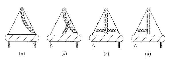
Figure 1: The one-loop renormalization of the three-parton correlation functions.

The central question is how to handle this unphysical pole when $k_{+}=0$. In the calculation of the relevant Feynman diagrams shown in Fig. 1 (and trivial self-energy insertions into external legs) we assume two different approaches, which employ the principal value (PV) and Mandelstam–Leibbrandt prescriptions (ML) [20]:

$${\rm PV}\frac{1}{k_{+}} = \frac{1}{2}\left\{\frac{1}{(kn)+i0}+\frac{1}{(kn)-i0}\right\},$$ (33)

$${\rm ML}\frac{1}{k_{+}} = \frac{(kn^{*})}{(kn)(kn^{*})+i0},$$ (34)

with the arbitrary four-vector $n^{*}$ satisfying $n^{*2}=0$, $nn^{*}=1$ (without loss of generality, we can put it equal to $p$). The first prescription will be used in the momentum space [9, 10, 21], the second one in the coordinate space formulation [13]. As a by-product we verify that both of them do lead to the same result.

In the light-cone fraction representation we get for the correlation function $D(x,x^{\prime})$:

$$\dot{D} (x,x^{\prime})=-\frac{\alpha}{2\pi}\Biggl{\{}-C_{F}\frac{(x-x^{\prime})}{xx^{\prime}}\left[x^{\prime}M(x)\Theta_{11}^{0}(x^{\prime},x^{\prime}-x)\pm xM(x^{\prime})\Theta_{11}^{0}(x,x-x^{\prime})\right]$$ (35)

$$+\int d\beta\Biggl{(}C_{F}D(\beta,x^{\prime})\frac{x}{x^{\prime}}\Theta_{11}^{0}(x,x-x^{\prime})+\frac{C_{A}}{2}\biggl{(}[D(\beta,x^{\prime})-D(x,x^{\prime})]\frac{x}{(x-\beta)}\Theta_{11}^{0}(x,x-\beta)$$

$$+[D(\beta+x^{\prime},x^{\prime})-D(x,x^{\prime})]\frac{(x-x^{\prime})}{(x-x^{\prime}-\beta)}\Theta_{11}^{0}(x-x^{\prime},x-x^{\prime}-\beta)$$

$$+\frac{(\beta+x-x^{\prime})}{x^{\prime}}\biggl{(}D(\beta,x^{\prime})\frac{x}{(x^{\prime}-x)}\Theta_{11}^{0}(x,x-\beta)+D(\beta+x^{\prime},x^{\prime})\Theta_{11}^{0}(x-x^{\prime},x-x^{\prime}-\beta)\biggr{)}\biggr{)}$$

$$+\left(C_{F}-\frac{C_{A}}{2}\right)\biggl{(}D(\beta,x^{\prime})\frac{(\beta+x-x^{\prime})}{(x^{\prime}-x)}\Theta_{111}^{0}(x,x-x^{\prime},x-x^{\prime}+\beta)$$

$$+[D(\beta,x^{\prime}-x+\beta)-D(x,x^{\prime})]\frac{x}{x-\beta}\Theta_{11}^{0}(x,x-\beta)\biggr{)}\Biggr{)}$$

$$+\int d\beta^{\prime}\Biggl{(}C_{F}D(x,\beta^{\prime})\frac{x^{\prime}}{x}\Theta_{11}^{0}(x^{\prime},x^{\prime}-x)+\frac{C_{A}}{2}\biggl{(}[D(x,\beta^{\prime})-D(x,x^{\prime})]\frac{x^{\prime}}{(x^{\prime}-\beta^{\prime})}\Theta_{11}^{0}(x^{\prime},x^{\prime}-\beta^{\prime})$$

$$+[D(x,\beta^{\prime}+x)-D(x,x^{\prime})]\frac{(x^{\prime}-x)}{(x^{\prime}-x-\beta^{\prime})}\Theta_{11}^{0}(x^{\prime}-x,x^{\prime}-x-\beta^{\prime})$$

$$+\frac{(\beta^{\prime}+x^{\prime}-x)}{x}\biggl{(}D(x,\beta^{\prime})\frac{x^{\prime}}{(x-x^{\prime})}\Theta_{11}^{0}(x^{\prime},x^{\prime}-\beta^{\prime})+D(x,\beta^{\prime}+x)\Theta_{11}^{0}(x^{\prime}-x,x^{\prime}-x-\beta^{\prime})\biggr{)}\biggr{)}$$

$$+\left(C_{F}-\frac{C_{A}}{2}\right)\biggl{(}D(x,\beta^{\prime})\frac{(\beta^{\prime}+x^{\prime}-x)}{(x^{\prime}-x)}\Theta_{111}^{0}(x^{\prime},x^{\prime}-x,x^{\prime}-x+\beta^{\prime})$$

$$+[D(x-x^{\prime}+\beta^{\prime},\beta^{\prime})-D(x,x^{\prime})]\frac{x^{\prime}}{x^{\prime}-\beta^{\prime}}\Theta_{11}^{0}(x^{\prime},x^{\prime}-\beta^{\prime})\biggr{)}\Biggr{)}-\frac{3}{2}C_{F}D(x,x^{\prime})\Biggr{\}},$$

and for the mass-dependent correlation function we have

$$\dot{M}(x)=-C_{F}\frac{\alpha}{2\pi}\int d\beta M(\beta)\left\{2\left[\frac{\beta}{(x-\beta)}\Theta_{11}^{0}(x,x-\beta)\right]_{+}+\frac{\beta+x}{\beta}\Theta_{11}^{0}(x,x-\beta)\right\},$$ (36)

where we have used the dot as short-hand for the logarithmic derivative with respect to the renormalization scale $\hskip 2.84544pt\dot{}=\mu_{R}^{2}\,{\partial}/{\partial\mu_{R}^{2}}$ and the standard plus-prescription fulfilling $\int dx[...]_{+}=0$ [for a definition see Eq. (B.4)]. The kernel of the last equation resembles the non-singlet splitting function of (un)polarized scattering up to the additional term $\frac{\alpha}{2\pi}\frac{3}{2}C_{F}\delta(x-\beta)$, which is the one-loop renormalization constant of the quark mass taken with a minus sign. An explicit form of the $\Theta$-functions is given in Appendix A. Throughout the paper the plus and minus signs in the mass-operator term correspond to the functions $D$ (for $e$) and $\widetilde{D}$ (for $h_{L}$), respectively.

For the string operators (or their matrix elements) we obtain the following compact RG equation:

$$\dot{\cal Z}(\lambda,\mu) = \frac{\alpha}{2\pi}\int_{0}^{1}dy\int_{0}^{\bar{y}}dz\biggl{\{}C_{F}{\bar{y}}^{2}\delta(z)\left[{\cal M}^{1}(\lambda-\mu y)\pm{\cal M}^{1}(\lambda y-\mu)\right]$$ (37)

$$+ \frac{C_{A}}{2}\left[2\bar{z}+[N(y,z)]_{+}-\frac{7}{4}\delta(\bar{y})\delta(z)\right]\left[{\cal Z}(\lambda y,\mu-\lambda z)+{\cal Z}(\lambda-\mu z,\mu y)\right]$$

$$+ \left(C_{F}-\frac{C_{A}}{2}\right)\biggl{[}\left[[L(y,z)]_{+}-\frac{1}{2}\delta(y)\delta(z)\right]{\cal Z}(\lambda\bar{z}+\mu z,\mu\bar{y}+\lambda y)$$

$$- 2z\left[{\cal Z}(-\lambda y,\mu-\lambda\bar{z})+{\cal Z}(\lambda-\mu\bar{z},-\mu y)\right]\biggr{]}\biggr{\}},$$

with

$$[N(y,z)]_{+}=N(y,z)-\delta(\bar{y})\delta(z)\int_{0}^{1}dy^{\prime}\int_{0}^{\bar{y}^{\prime}}dz^{\prime}N(y^{\prime},z^{\prime}),\hskip 14.22636ptN(y,z)=\delta(\bar{y}-z)\frac{y^{2}}{\bar{y}}+\delta(z)\frac{y}{\bar{y}},$$

$$[L(y,z)]_{+}=L(y,z)-\delta(y)\delta(z)\int_{0}^{1}dy^{\prime}\int_{0}^{\bar{y}^{\prime}}dz^{\prime}L(y^{\prime},z^{\prime}),\hskip 14.22636ptL(y,z)=\delta(y)\frac{\bar{z}}{z}+\delta(z)\frac{\bar{y}}{y}.$$ (38)

The equations written so far should be supplemented by the following

$$\dot{\cal M}^{1}(\lambda) = \frac{\alpha}{2\pi}C_{F}\int_{0}^{1}dy\left\{\left[\frac{2}{\bar{y}}\right]_{+}-2-y-y^{2}\right\}{\cal M}^{1}(\lambda y),$$ (39)

$$\dot{h}_{1}(\lambda) = \frac{\alpha}{2\pi}C_{F}\int_{0}^{1}dy\left\{\left[\frac{2}{\bar{y}}\right]_{+}-2+\frac{3}{2}\delta(\bar{y})\right\}h_{1}(\lambda y).$$ (40)

The last one, when transformed to the momentum space using the formulae of the next section, coincides with the result obtained in Ref. [22].

3 From light-cone position to light-cone fraction
representations

Having at hand the evolution equations in different representations for the same quantities, it is instructive to relate the kernels in both cases. Such a bridge can be easily established using the Fourier transformation for the parton distribution functions given by Eqs. (2) and (4).

First, we come to the simpler case of the two-particle correlation functions ${\cal F}$. The evolution equation in the light-cone position space is of the following generic form

$$\dot{\cal F}(\lambda)=\int_{0}^{1}dy{\cal K}(y){\cal F}(\lambda y),$$ (41)

where ${\cal K}(y)$ is an evolution kernel in the coordinate space. By exploiting the definitions (2) we can recast the Fourier transform on the language of two-particle evolution kernels. In this way we find the direct transformation

$$K(x,\beta)=\int_{0}^{1}dy{\cal K}(y)\delta(x-y\beta).$$ (42)

And using the general formula

$$\int_{0}^{1}dyf(y)\delta(x-y\beta)=f\left(\frac{x}{\beta}\right)\Theta^{0}_{11}(x,x-\beta).$$ (43)

with the familiar $\Theta$-function of the momentum space formulation, we can observe that the RG equations for two-parton correlators derived in the previous section indeed coincide. The inverse transformation can be done

$$\int\frac{dxd\beta}{2\pi}e^{-i\lambda x+i\mu\beta}K(x,\beta)=\int_{0}^{1}dy{\cal K}(y)\delta(\mu-y\lambda)$$ (44)

with the help of the formula

$$\int\frac{dxd\beta}{2\pi}f\left(\frac{x}{\beta}\right)\Theta^{0}_{11}(x,x-\beta)e^{-i\lambda x+i\mu\beta}=\int_{0}^{1}dyf(y)\delta(\mu-y\lambda).$$ (45)

The corresponding transformation for three-particle correlators is a little bit more involved. The general form of the evolution equation for the light-cone string operator ${\cal Z}(\lambda,\mu)$ reads

$$\dot{\cal Z}(\lambda,\mu)=\int_{0}^{1}dy\int_{0}^{\bar{y}}dz{\cal K}(y,z){\cal Z}(\eta_{11}\lambda+\eta_{12}\mu,\eta_{21}\lambda+\eta_{22}\mu),$$ (46)

where $\eta_{ij}$ are linear functions of the variables $y$, $z$. In the momentum fraction representation the evolution equation looks like

$$\dot{Z}(x,x^{\prime})=\int d\beta d\beta^{\prime}K(x,x^{\prime},\beta,\beta^{\prime})Z(\beta,\beta^{\prime}).$$ (47)

Specifying the particular form of the functions $\eta_{ij}$, we list below the corresponding conversion formulae.

For the $C_{A}/2$ part of the evolution equation, the Fourier transformation gives

$$K(x,x^{\prime},\beta,\beta^{\prime})=\delta(\beta^{\prime}-x^{\prime})\int_{0}^{1}dy\int_{0}^{\bar{y}}dz{\cal K}(y,z)\delta(x-x^{\prime}z-\beta y).$$ (48)

The particular contributions are

$${\cal K}_{1}(y,z)=\delta(\bar{y})\delta(z)\ \stackrel{{\scriptstyle FT}}{{\rightarrow}}\ K_{1}(x,x^{\prime},\beta,\beta^{\prime})=\delta(\beta-x)\delta(\beta^{\prime}-x^{\prime}),$$ (49)

$${\cal K}_{2}(y,z)=\delta(z)\frac{y}{\bar{y}}+\delta(\bar{y}-z)\frac{y^{2}}{\bar{y}}\ \stackrel{{\scriptstyle FT}}{{\rightarrow}}\ K_{2}(x,x^{\prime},\beta,\beta^{\prime})=\delta(\beta^{\prime}-x^{\prime})\biggl{\{}\frac{x}{\beta-x}\Theta^{0}_{11}(x,x-\beta)$$

$$\hskip 221.93158pt+\frac{(x-x^{\prime})^{2}}{(\beta-x)(\beta-x^{\prime})}\Theta^{0}_{11}(x-x^{\prime},x-\beta)\biggr{\}},$$ (50)

$${\cal K}_{3}(y,z)=1\ \stackrel{{\scriptstyle FT}}{{\rightarrow}}\ K_{3}(x,x^{\prime},\beta,\beta^{\prime})=\delta(\beta^{\prime}-x^{\prime})\Xi_{1}(x,x-x^{\prime},x-\beta)$$

$$\hskip 221.93158pt=-\delta(\beta^{\prime}-x^{\prime})\Theta^{0}_{111}(x,x-x^{\prime},x-\beta),$$ (51)

$${\cal K}_{4}(y,z)=z\ \stackrel{{\scriptstyle FT}}{{\rightarrow}}\ K_{4}(x,x^{\prime},\beta,\beta^{\prime})=\delta(\beta^{\prime}-x^{\prime})\biggl{\{}\frac{x-\beta}{x^{\prime}}\Xi_{1}(x,x-x^{\prime},x-\beta)$$

$$\hskip 221.93158pt+\frac{\beta}{x^{\prime}}\Xi_{2}(x,x-x^{\prime},x-\beta)\biggr{\}}.$$ (52)

Here we have used (43) and the following useful formula

$$\Xi_{n}(x,x-x^{\prime},x-\beta)\equiv\int_{0}^{1}dyy^{n}\Theta^{0}_{11}((x-\beta)+y\beta,(x-\beta)-y(x^{\prime}-\beta))$$

$$=\frac{1}{n}\left[1-\left(\frac{\beta-x}{\beta-x^{\prime}}\right)^{n}\right]\Theta^{0}_{11}(x,x-x^{\prime})+\frac{1}{n}\frac{\beta}{x^{\prime}}\left[\left(\frac{\beta-x}{\beta-x^{\prime}}\right)^{n}-\left(\frac{\beta-x}{\beta}\right)^{n}\right]\Theta^{0}_{11}(x,x-\beta).$$ (53)

The analogous results for the $(C_{F}-C_{A}/2)$ part of the kernel read

$$K(x,x^{\prime},\beta,\beta^{\prime})=\delta(\beta^{\prime}-x^{\prime})\int_{0}^{1}dy\int_{0}^{\bar{y}}dz{\cal K}(y,z)\delta(x-x^{\prime}\bar{z}+\beta y),$$ (54)

and in particular

$${\cal K}_{1}(y,z)=z\ \stackrel{{\scriptstyle FT}}{{\rightarrow}}\ K_{1}(x,x^{\prime},\beta,\beta^{\prime})=\delta(\beta^{\prime}-x^{\prime})\biggl{\{}\frac{x^{\prime}-x-\beta}{x^{\prime}}\Xi_{1}(x^{\prime}-x,-x,x^{\prime}-x-\beta)$$

$$\hskip 221.93158pt+\frac{\beta}{x^{\prime}}\Xi_{2}(x^{\prime}-x,-x,x^{\prime}-x-\beta)\biggr{\}}.$$ (55)

In addition, we have

$$K(x,x^{\prime},\beta,\beta^{\prime})=\int_{0}^{1}dy\int_{0}^{\bar{y}}dz{\cal K}(y,z)\delta(x-\beta\bar{z}+\beta^{\prime}y)\delta(x^{\prime}-\beta^{\prime}\bar{y}+\beta z)$$ (56)

and

$${\cal K}_{1}(y,z)=\delta(z)\frac{\bar{y}}{y}\ \stackrel{{\scriptstyle FT}}{{\rightarrow}}\ K_{1}(x,x^{\prime},\beta,\beta^{\prime})=\delta(\beta-(\beta^{\prime}-x^{\prime}+x))\frac{x^{\prime}}{\beta^{\prime}-x^{\prime}}\Theta^{0}_{11}(x^{\prime},x^{\prime}-\beta^{\prime}).$$ (57)

These formulae complete the list of transformations. Collecting particular contributions, we can easily verify that the evolution equations given by Eqs. (35) and (37) agree with each other. It should be noted that it is sufficient to have at hand Eqs. (43) and (3) to perform the conversion from one representation to another.

4 Generalized DGLAP-type equations

To study the large-$N_{c}$ limit and establish the relation to the evolution equation for the partially Mellin-transformed operators introduced in Refs. [11, 14, 16], we proceed to the generalized DGLAP representation of the evolution equation for three-particles distributions first given in the second paper of Ref. [13]. For this purpose we define a new function, Fourier-transformed with respect to the $\lambda$ variable only:

$${\scriptstyle\cal Z}(x,u)=\frac{1}{2}\int\frac{d\lambda}{2\pi}e^{i\lambda x}\langle h|{\cal Z}(\bar{u}\lambda,-u\lambda)\pm(u\to\bar{u})|h\rangle,$$ (58)

which is even under charge conjugation and depends on the variables $x$ and $u$. The latter has the meaning of the relative position of the gluon field on the light cone. For $0\leq u\leq 1$ the gluon field lies between the two quark fields. Because of the support property $|x|\leq{\rm max}(1,|2u-1|)$, the variable $x$ is then restricted to $|x|\leq 1$ and can be interpreted as an effective momentum fraction.

The evolution equation for ${\scriptstyle\cal Z}(x,u)$ can be derived in a straightforward way from the RG equation (37) for the non-local string operator ${\cal Z}$. It can be presented in the form of a generalized DGLAP-type equation:

$$\dot{\scriptstyle\cal Z}\left(x,u\right) = \frac{\alpha_{s}}{2\pi}\int\frac{dy}{y}\int dv\Bigg{\{}P_{{\scriptscriptstyle\cal ZZ}}(y,u,v){\scriptstyle\cal Z}\left(\frac{x}{y},v\right)+P_{{\scriptscriptstyle\cal Z}m}(y,u,v)m\left(\frac{x}{v}\right)\Bigg{\}},$$ (59)

$$\dot{m}(x) = \frac{\alpha_{s}}{2\pi}\int\frac{dy}{y}P_{mm}(y)m\left(\frac{x}{y}\right).$$ (60)

Here, $m(x)=xM(x)$ and the integration region is determined both by the support of ${\scriptstyle\cal Z}(x,u)$ and by the kernels

$$P_{\scriptscriptstyle\cal ZZ}(x,u,v)$$

$$=\left(C_{F}-\frac{C_{A}}{2}\right)\Bigg{[}{\mit\Theta}_{1}(x,u,v)[L(x,u,v)]_{+}-{\mit\Theta}_{2}(x,u,v)M(x,u,v)-{1\over 4}\delta(u-v)\delta(\bar{x})\Bigg{]}$$

$$+\frac{C_{A}}{2}{\mit\Theta}_{3}(x,u,v)\left[M(x,u,v)+[N(x,u,v)]_{+}-\frac{7}{4}\delta(u-v)\delta(\bar{x})\right]+{u\rightarrow\bar{u}\choose v\rightarrow\bar{v}},$$ (61)

$$P_{{\scriptscriptstyle\cal Z}m}(x,u,v)=C_{F}{\bar{x}}^{2}\theta(x)\theta(\bar{x})\frac{x}{v}\left[\delta(v-\bar{u}-xu)\pm\delta(v-u-x\bar{u})\right],$$ (62)

$$P_{mm}(x)=C_{F}\left[\left[\frac{2}{\bar{x}}\right]_{+}-2-x-x^{2}\right],$$ (63)

where the auxiliary functions are defined by:

$${\mit\Theta}_{1}(x,u,v) = \theta(x)\theta(u-xv)\theta(\bar{u}-x\bar{v}),$$

$${\mit\Theta}_{2}(x,u,v) = \theta\left(-\frac{x\bar{v}}{\bar{u}}\right)\theta\left(\frac{1-xv}{\bar{u}}\right)\theta\left(\frac{x-u}{\bar{u}}\right),$$

$${\mit\Theta}_{3}(x,u,v) = \theta\left(\frac{\bar{x}}{\bar{u}}\right)\theta\left(\frac{x\bar{v}}{\bar{u}}\right)\theta\left(\frac{xv-u}{\bar{u}}\right),$$

$$L(x,u,v) = \frac{u^{2}}{v(v-u)}\delta(u-xv),$$

$$M(x,u,v) = \frac{2x(1-xv)}{{\bar{u}}^{3}},$$

$$N(x,u,v) = \frac{\bar{v}\epsilon(\bar{u})}{\bar{u}(v-u)}\left[\frac{\bar{v}}{\bar{u}}\delta(\bar{x})+\frac{u^{2}}{v}\delta(u-xv)\right].$$ (64)

The plus-prescription for the arbitrary function $A$ is defined by the equation

$${\mit\Theta}_{i}(x,u,v)[A(x,u,v)]_{+}$$

$$={\mit\Theta}_{i}(x,u,v)A(x,u,v)-\delta(\bar{x})\delta(u-v)\int_{0}^{1}dx^{\prime}\int dv^{\prime}\,{\mit\Theta}_{i}(x^{\prime},u,v^{\prime})A(x^{\prime},u,v^{\prime}).$$ (65)

Note that, due to the evolution, the variable $u$ is no longer restricted to the region $0\leq u\leq 1$.

Going further, we introduce the Mellin transforms

$${\scriptstyle\cal Z}^{n}(u)=\int dxx^{n-1}{\scriptstyle\cal Z}(x,u)\hskip 14.22636pt\mbox{and}\hskip 14.22636ptm^{n}=\int dxx^{n-1}m(x)=\int dx\,x^{n}M(x),$$ (66)

where $n$ is the complex angular momentum. Operators with different $n$ do not mix with each other and satisfy the evolution equations

$$\dot{\scriptstyle\cal Z}^{n}(u) = \frac{\alpha_{s}}{2\pi}\int dv\left\{P^{n}_{{\scriptscriptstyle\cal ZZ}}(u,v){\scriptstyle\cal Z}^{n}(v)+\delta(u-v)\left[P^{n}_{{\scriptscriptstyle\cal Z}m}(v)\pm P^{n}_{{\scriptscriptstyle\cal Z}m}(\bar{v})\right]m^{n}\right\},$$ (67)

$$\dot{m}^{n} = \frac{\alpha_{s}}{2\pi}P_{mm}^{n}m^{n}.$$ (68)

The kernels are given by

$$P^{n}_{{\scriptscriptstyle\cal ZZ}}(u,v)=\left(C_{F}-\frac{C_{A}}{2}\right)\Bigg{[}{\mit\Theta}_{1}(u,v)[L^{n}(u,v)]_{+}-{\mit\Theta}_{2}(u,v)M^{n}_{1}(u,v)-\frac{1}{4}\delta(u-v)\Bigg{]}$$

$$+\frac{C_{A}}{2}{\mit\Theta}_{3}(u,v)\left[M^{n}_{2}(u,v)+[N^{n}(u,v)]_{+}-\frac{7}{4}\delta(u-v)\right]+{u\rightarrow\bar{u}\choose v\rightarrow\bar{v}},$$

$$P^{n}_{{\scriptscriptstyle\cal Z}m}(v)=C_{F}\frac{2-{\bar{v}}^{n}[2+n(2+(n+1)v)v]}{n(n+1)(n+2)v^{3}},$$

$$P^{n}_{mm}=-C_{F}\left(S_{n}+S_{n+2}\right),$$ (69)

where the auxiliary functions read

$${\mit\Theta}_{1}(u,v)=\theta(v-u),\quad{\mit\Theta}_{2}(u,v)=\theta(-\bar{v})\theta(1-vu),\quad{\mit\Theta}_{3}(u,v)=\theta(\bar{v})\theta(v-u).$$ (70)

$$L^{n}(u,v) = \frac{\epsilon(v)}{v-u}\left(\frac{u}{v}\right)^{n+1},$$

$$M_{1}^{n}(u,v) = \frac{2}{{\bar{u}}^{3}}\left\{\frac{1}{n+1}\left[\frac{1}{v^{n+1}}-u^{n+1}\right]-\frac{v}{n+2}\left[\frac{1}{v^{n+2}}-u^{n+2}\right]\right\},$$

$$M_{2}^{n}(u,v) = \frac{2}{{\bar{u}}^{3}}\left\{\frac{1}{n+1}\left[1-\left(\frac{u}{v}\right)^{n+1}\right]-\frac{v}{n+2}\left[1-\left(\frac{u}{v}\right)^{n+2}\right]\right\},$$

$$N^{n}(u,v) = \frac{\bar{v}\epsilon(\bar{u})}{\bar{u}(v-u)}\left\{\frac{\bar{v}}{\bar{u}}+\epsilon(v)\left(\frac{u}{v}\right)^{n+1}\right\}.$$ (71)

The plus-prescription is defined as

$${\mit\Theta}_{i}(u,v)[A^{n}(u,v)]_{+}={\mit\Theta}_{i}(u,v)A^{n}(u,v)-\delta(u-v)\int dv^{\prime}{\mit\Theta}_{i}(u,v^{\prime})A^{n}(u,v^{\prime}).$$ (72)

It is not difficult to observe that, in multicolour limit, Eq. (67) is exactly reduced to the equation of Ref. [16], which was the starting point of their analysis. However, we will start from Eq. (59) in the mixed representation and show in the next section that in the multicolour limit the generalized splitting functions can be diagonalized.

5 Solution of the evolution equations in multicolour QCD

This section is devoted to the solution of the evolution equations we derived in the previous sections for the twist-3 correlation functions. First of all, we perform an extensive numerical study of the exact Eq. (67). For simplicity we restrict ourselves to the homogeneous case, i.e.  we discard the quark-mass operator, which is certainly a justified assumption for the light $u$- and $d$-quark species. The solution we are interested in is given in terms of the eigenvalues and eigenfunctions of the anomalous-dimension matrix ${}_{\scriptscriptstyle ZZ}\gamma_{n}^{l}$ of the local operators ${\cal Z}_{n}^{l}$ calculated in Appendix C. The eigenvalue problem we have attacked has no analytical solution; however, the diagonalization can be done numerically for moderately large orbital momentum $n$, e.g.  $n\leq 100$, which is quite sufficient for practical purposes. Second, we provide the analytical solution of the generalized DGLAP equation in the multicolour limit of QCD. In this case it reduces to the familiar ladder-type equation that holds for the twist-2 operators. It will be shown that such a reduction occurs in the limit $x\to 1$ too. Assembling the two results allows us to construct the improved DGLAP-type equations for two-quark twist-3 distributions. Exploiting some examples of the evolution for the moments, we confront these two approaches. In particular, we study the accuracy of the improved DGLAP equation with respect to the exact evolution for different models of gluon light-cone position distribution for the three-particle correlation function at low momentum scale.

5.1 Evolution of the moments

To obtain the solution of the evolution equation (67) we choose $n$ as a positive integer. In this case, as follows from the definition (58) of ${\scriptstyle\cal Z}^{n}(u)$ the $n$-th moment is actually given by the following linear combination of local operators ${\cal Z}_{n}^{l}$ (see Eq. (C.1)):

$${\scriptstyle\cal Z}^{n}(u)=\sum_{l=1}^{n}C_{n-1}^{l-1}\,u^{n-l}{\bar{u}}^{l-1}{\cal Z}_{n}^{l},$$ (73)

so that ${\scriptstyle\cal Z}^{n}(u)$ is a polynomial of degree $n-1$ in $u$. Thus the kernel $P^{n}_{{\scriptscriptstyle\cal ZZ}}(u,v)$ possesses $n$ polynomial eigenfunctions $e^{n}_{l}(v)$:

$$\int dv\,P^{n}_{{\scriptscriptstyle\cal ZZ}}(u,v)e^{n}_{l}(v)=-\lambda^{n}_{l}e^{n}_{l}(u),\quad l=1,\dots,n,$$ (74)

where $-\lambda^{n}_{l}$ denotes the eigenvalues. These eigenfunctions can be constructed by diagonalization

$$C_{n-1}^{k-1}\int dv\,P^{n}_{{\scriptscriptstyle\cal ZZ}}(u,v)v^{n-k}\bar{v}^{k-1} = \sum_{l=1}^{n}C_{n-1}^{l-1}{{}_{\scriptscriptstyle ZZ}\gamma}^{n}_{lk}\,u^{n-l}\bar{u}^{l-1},$$ (75)

where the anomalous-dimension matrix ${{}_{\scriptscriptstyle ZZ}\gamma}^{n}_{lk}$ of the local operators is given by Eq. (C.13). Actually, this is a purely algebraic task and we find

$$e^{n}_{k}(u)=\sum_{l=1}^{n}C_{n-1}^{l-1}\,u^{n-l}\bar{u}^{l-1}E^{n}_{lk},\mbox{\ with\ }\left\{(E^{n})^{-1}{{}_{\scriptscriptstyle ZZ}\gamma}^{n}E^{n}\right\}_{kl}=-\lambda^{n}_{k}\delta(k-l),$$ (76)

where $\delta(k-l)$ is a Kronecker symbol defined by Eq. (C.14). The spectrum of the eigenvalues $\lambda^{n}_{l}$ up to $n=50$ is shown in Fig. 2a, together with some examples of the eigenfunctions of the kernel $P^{n}_{\scriptscriptstyle\cal ZZ}$ for particular orbital momenta. The solution for the moments ${\scriptstyle\cal Z}^{n}(u)$ (in the massless case) is then expressed in terms of the eigenfunctions and eigenvalues we have found:

$${\scriptstyle\cal Z}^{n}\left(u,Q^{2}\right)=\sum_{l=1}^{n}c^{n}_{l}\left(Q_{0}^{2}\right)e^{n}_{l}(u)\exp{\left\{-\int_{Q_{0}^{2}}^{Q^{2}}\frac{dt}{t}\frac{\alpha_{s}(t)}{2\pi}\lambda^{n}_{l}\right\}}.$$ (77)

The coefficients $c^{n}_{l}\left(Q_{0}^{2}\right)$ at the reference momentum squared $Q^{2}_{0}$ have to be determined from the non-perturbative input ${\scriptstyle\cal Z}^{n}\left(u,Q_{0}^{2}\right)$:

$$c^{n}_{l}\left(Q_{0}^{2}\right)=\sum_{k=1}^{n}(E^{n}_{lk})^{-1}\frac{(n-k)!}{(n-1)!}\frac{d^{k-1}}{dw^{k-1}}(1+w)^{n-1}{\scriptstyle\cal Z}^{n}\left({1\over 1+w},Q_{0}^{2}\right)_{|w=0}.$$ (78)

5.2 Reduction of the evolution equations

In the large-$N_{c}$ limit only the planar diagrams (Fig. 1 a, d) survive and the kernel $P^{n}_{\scriptscriptstyle\cal ZZ}(u,v)$ has two known dual eigenfunctions: $1$ and $1-2u$, so that $\int_{0}^{1}du\,e^{n}_{l}(u)=\delta_{l1}+{\cal O}(1/N_{c})$ and $\int_{0}^{1}du\,(1-2u)e^{n}_{l}(u)=\delta_{l2}+{\cal O}(1/N_{c})$, where $l=1,2$ correspond to the lowest two eigenvalues of the spectrum shown in Fig. 2a. A straightforward calculation gives the following DGLAP evolution kernels:

$$\int_{0}^{1}du\,\!\left\{\!\begin{array}[]{c}1\\ \frac{1-2u}{1-2v}\end{array}\!\right\}P_{\scriptscriptstyle\cal ZZ}(x,u,v)=N_{c}\,\theta(\bar{x})\theta(x)\!\left\{\!\begin{array}[]{c}\left[\frac{x^{2}}{\bar{x}}\right]_{+}+\frac{1}{2}x^{2}-\frac{5}{4}\delta(\bar{x})\\ \left[\frac{x^{2}}{\bar{x}}\right]_{+}-\frac{3}{2}x^{2}-\frac{5}{4}\delta(\bar{x})\end{array}\!\right\}+{\cal O}\left(\frac{1}{N_{c}}\right),$$ (79)

and for the mass-mixing kernels the exact results read

$$\int_{0}^{1}du\,\!\left\{\!\begin{array}[]{c}1\\ \frac{1-2u}{1-2v}\end{array}\!\right\}P_{{\scriptscriptstyle\cal Z}m}(x,u,v)=C_{F}\,\theta(\bar{x})\theta(x)\!\left\{\!\begin{array}[]{c}x(2-x)\\ 0\end{array}\!\right\}\quad\mbox{for e},$$ (84)

$$\int_{0}^{1}du\!\left\{\!\begin{array}[]{c}1\\ \frac{1-2u}{1-2v}\end{array}\!\right\}P_{{\scriptscriptstyle\cal Z}m}(x,u,v)=C_{F}\,\theta(\bar{x})\theta(x)\!\left\{\!\begin{array}[]{c}0\\ x(2-3x)\end{array}\!\right\}\quad\mbox{for $\widetilde{h}_{L}$}.$$ (89)

As was first observed in Ref. [14] in the context of the chiral-even distribution $g_{2}(x)$, similar equations hold true also for the $\frac{1}{N_{c}}$-suppressed terms in the $x\to 1$ limit for flavour non-singlet twist-3 evolution kernels. In the present chiral-odd case, we find

$$\int_{0}^{1}du\,\!\left\{\!\begin{array}[]{c}1\\ \frac{1-2u}{1-2v}\end{array}\!\right\}P_{\scriptscriptstyle\cal ZZ}(x,u,v)=-\frac{1}{N_{c}}\theta(\bar{x})\theta(x)\!\left\{\!\begin{array}[]{c}\left[\frac{1}{\bar{x}}\right]_{+}+\frac{5}{4}\delta(\bar{x})+{\cal O}(\bar{x}^{0})\\ \left[\frac{1}{\bar{x}}\right]_{+}+\frac{19}{12}\delta(\bar{x})+{\cal O}(\bar{x}^{0})\end{array}\!\right\}+N_{c}\cdots,$$ (94)

where the $N_{c}\cdots$ symbolize the $x\to 1$ limit of Eq. (79).

The eigenfunctions we have obtained coincide precisely with the coefficients that appear in the decomposition of $e(x,Q^{2})$ and $\widetilde{h}_{L}(x,Q^{2})$ in terms of three-particle correlation functions. To observe this explicitly we need relations similar to the ones given by Eqs. (10) and (30) transformed to the mixed representation (58). Namely, we have

$$e(x) = \frac{1}{x}m(x)-\frac{1}{2}\frac{d}{dx}\int_{0}^{1}du\,{\scriptstyle\cal Z}(x,u),$$ (95)

$$\bar{h}_{L}(x) = \frac{1}{x}\widetilde{m}(x)-\frac{1}{2}\frac{d}{dx}\int_{0}^{1}du\,(1-2u)\widetilde{\scriptstyle\cal Z}(x,u),$$ (96)

where we introduce for convenience a new function $\bar{h}_{L}(x)$, so that ${h}_{L}(x)$ reads:

$${h}_{L}(x)=2\int_{x}^{1}dy\,\frac{x^{2}}{y^{2}}h_{1}(y)-x\frac{d}{dx}\int_{x}^{1}\frac{dy}{y}\frac{x^{2}}{y^{2}}\bar{h}_{L}(y).$$ (97)

For the massless case the last term on the RHS coincides with the twist-3 part $\widetilde{h}_{L}$.

From the observations we have made above, it follows that in the large-$N_{c}$ as well as in the large-$x$ limit the twist-3 distributions satisfy the DGLAP evolution equations. By combining the large-$N_{c}$ evolution with the large-$x$ result for the $\frac{1}{N_{c}}$-suppressed terms, we can improve the accuracy of such an approximation within a factor 5–10, to be compared with the multicolour limit taken alone (see Fig. 2b). Thus, the functions $e(x,Q^{2})$ and ${\bar{h}}_{L}(x,Q^{2})$ obey the following improved evolution equations:

$$\left\{\begin{array}[]{c}\dot{e}(x)\\ {\dot{\bar{h}}}_{L}(x)\end{array}\right\}={\alpha_{s}\over 2\pi}\int_{x}^{1}\frac{dy}{y}\left\{\begin{array}[]{c}P_{ee}(y)\,e\left(\frac{x}{y}\right)+\left[\frac{1}{x}\left\{P_{mm}(y)-P_{ee}(y)\right\}-\frac{1}{2}P_{em}(y)\frac{d}{dx}\right]m\left(\frac{x}{y}\right)\\ P_{\bar{h}\bar{h}}(y)\,{\bar{h}}_{L}\left(\frac{x}{y}\right)+\left[\frac{1}{x}\left\{P_{mm}(y)-P_{\bar{h}\bar{h}}(y)\right\}-\frac{1}{2}P_{\bar{h}m}(y)\frac{d}{dx}\right]m\left(\frac{x}{y}\right)\end{array}\right\},$$ (102)

with

$$P_{ee}(y)=2C_{F}\left[\frac{y}{\bar{y}}\right]_{+}+\frac{C_{A}}{2}y+\left(\frac{C_{F}}{2}-C_{A}\right)\delta(\bar{y})+{\cal O}\left({\bar{y}}^{0}/N_{c}\right),$$

$$P_{\bar{h}\bar{h}}(y)=2C_{F}\left[\frac{y}{\bar{y}}\right]_{+}-\frac{3C_{A}}{2}y+\left(\frac{7C_{F}}{6}-\frac{4C_{A}}{3}\right)\delta(\bar{y})+{\cal O}\left({\bar{y}}^{0}/N_{c}\right),$$ (103)

$$P_{em}(y)=C_{F}x(2-x),$$

$$P_{\bar{h}m}(y)=C_{F}x(2-3x).$$ (104)

The evolution kernel for the mass-dependent correlator was already given by Eq. (63). In Eq. (5.2) we have added subleading terms ${\cal O}\left({\bar{y}}^{0}/N_{c}\right)$ (which we do not specify here) so that the first moment of each kernel coincides with the corresponding eigenvalue of the kernel $P^{n}_{{\scriptscriptstyle\cal ZZ}}(u,v)$. This guarantees that the solution for the lowest moments given below, in Eq. (5.3), will be reproduced exactly. Note that in the massless case $\widetilde{{h}}_{L}(x)$ fulfills the same evolution equation as ${\bar{h}}_{L}(x)$. The simplest way to verify this is to make the Mellin transform of the corresponding evolution equations.

Let us add a few remarks on the momentum space formulation. As we have seen above the solution of the evolution equations in the asymptotic regimes is the most straightforward in the light-cone position representation. It is by no means trivial to observe the appearance of the DGLAP equations in momentum fraction representation. However, we know that the asymptotic solution, in coordinate space, is given by the convolution of the three-particle correlation function with the same weight function that enters in the decomposition of the two-parton correlators at tree level. With this in mind, we are able to check that the integrals

$$e(x) = \int d\beta^{\prime}D(x,\beta^{\prime}),$$ (105)

$$\widetilde{h}_{L}(x) = x^{2}\int_{x}^{1}\frac{d\beta}{\beta^{2}}\int\frac{d\beta^{\prime}}{\beta^{\prime}-\beta}\left\{2+(\beta-\beta^{\prime})\left[\frac{\partial}{\partial\beta}-\frac{\partial}{\partial\beta^{\prime}}\right]\right\}\widetilde{D}(\beta,\beta^{\prime}),$$ (106)

taken from Eqs. (10) and (30) neglecting quark-mass as well as twist-2 effects, satisfy the DGLAP equations, namely

$$\dot{e}(x)$$

$$=-\frac{\alpha}{4\pi}N_{c}\int d\beta e(\beta)\left\{2\left[\frac{\beta}{(x-\beta)}\Theta_{11}^{0}(x,x-\beta)\right]_{+}+\left(2-\frac{x}{\beta}\right)\Theta_{11}^{0}(x,x-\beta)-\frac{1}{2}\delta(\beta-x)\right\},$$ (107)

$$\dot{\widetilde{h}}_{L}(x)$$

$$=-\frac{\alpha}{4\pi}N_{c}\int d\beta\widetilde{h}_{L}(\beta)\left\{2\left[\frac{\beta}{(x-\beta)}\Theta_{11}^{0}(x,x-\beta)\right]_{+}+\left(2+3\frac{x}{\beta}\right)\Theta_{11}^{0}(x,x-\beta)-\frac{1}{2}\delta(\beta-x)\right\}.$$ (108)

The corresponding anomalous dimensions are

$$\dot{[e]}_{n} = \frac{\alpha}{4\pi}N_{c}\left\{-2\psi(n+2)-2\gamma_{E}+\frac{1}{2}+\frac{1}{n+2}\right\}[e]_{n},$$ (109)

$$\dot{[\widetilde{h}_{L}]}_{n} = \frac{\alpha}{4\pi}N_{c}\left\{-2\psi(n+2)-2\gamma_{E}+\frac{1}{2}-\frac{3}{n+2}\right\}[\widetilde{h}_{L}]_{n}.$$ (110)

Which are exactly the anomalous dimensions $\gamma^{\pm}_{n}$ found in Ref. [16] for $e$ and $h_{L}$, respectively, with the replacement $n\to j-1$ .

5.3 Examples of the evolution

For the lowest few moments the evolution equation (67) can be solved exactly. Taking into account the symmetry properties of the quark–gluon correlation function, we obtain the following results for the (non-vanishing) first two moments:

$${\scriptstyle\cal Z}^{1}\left(u,Q^{2}\right) = {\scriptstyle\cal Z}^{1}\left(Q_{0}^{2}\right)\exp\left\{-\frac{55}{18}\int_{Q_{0}^{2}}^{Q^{2}}\frac{dt}{t}\frac{\alpha_{s}(t)}{2\pi}\right\},$$

$${\scriptstyle\cal Z}^{2}\left(u,Q^{2}\right) = {\scriptstyle\cal Z}^{2}\left(Q_{0}^{2}\right)\exp\left\{-\frac{73}{18}\int_{Q_{0}^{2}}^{Q^{2}}\frac{dt}{t}\frac{\alpha_{s}(t)}{2\pi}\right\}$$

$$\widetilde{\scriptstyle\cal Z}^{2}\left(u,Q^{2}\right) = \widetilde{\scriptstyle\cal Z}^{2}\left(Q_{0}^{2}\right)(1-2u)\exp\left\{-\frac{52}{9}\int_{Q_{0}^{2}}^{Q^{2}}\frac{dt}{t}\frac{\alpha_{s}(t)}{2\pi}\right\},$$

$$\widetilde{\scriptstyle\cal Z}^{3}\left(u,Q^{2}\right) = \widetilde{\scriptstyle\cal Z}^{3}\left(Q_{0}^{2}\right)(1-2u)\exp\left\{-\frac{1099}{180}\int_{Q_{0}^{2}}^{Q^{2}}\frac{dt}{t}\frac{\alpha_{s}(t)}{2\pi}\right\},$$ (111)

where ${\scriptstyle\cal Z}^{n}\left(Q_{0}^{2}\right)$ are related to the following matrix elements of the local operators (up to normalization)

$${\scriptstyle\cal Z}^{1}\left(Q_{0}^{2}\right) = Z^{1}_{1}\left(Q_{0}^{2}\right)=\langle h|{\cal Z}^{1}_{1}|h\rangle_{|\mu^{2}=Q_{0}^{2}},\quad{\scriptstyle\cal Z}^{2}\left(Q_{0}^{2}\right)=Z^{1}_{2}\left(Q_{0}^{2}\right)=\langle h|{\cal Z}^{1}_{2}|h\rangle_{|\mu^{2}=Q_{0}^{2}},$$

$$\widetilde{\scriptstyle\cal Z}^{2}\left(Q_{0}^{2}\right) = \widetilde{Z}^{1}_{2}\left(Q_{0}^{2}\right)=\langle h|\widetilde{\cal Z}^{1}_{2}|h\rangle_{|\mu^{2}=Q_{0}^{2}},\quad\widetilde{\scriptstyle\cal Z}^{3}\left(Q_{0}^{2}\right)=\widetilde{Z}^{1}_{3}\left(Q_{0}^{2}\right)=\langle h|\widetilde{\cal Z}^{1}_{3}|h\rangle_{|\mu^{2}=Q_{0}^{2}}.$$ (112)

Thus the $Q^{2}$-dependence for the first moments of $e(x)$ and $\widetilde{h}_{L}(x)$ can be predicted uniquely since the initial values at the low-momentum scale are given by these moments themselves. For larger $n$, the evolution is sensitive to the shape of the gluon distribution between the quark fields. However, as can be traced from Figs. 3 and 4, the dependence on the assumed different toy models of the light-cone position distribution at $Q_{0}^{2}=1\mbox{\ }{\rm GeV}^{2}$ is quite small: the typical relative deviations for the moments of the twist-3 unpolarized and polarized structure functions are $2\%$ and $5\%$, respectively, at $Q^{2}=100\mbox{\ }{\rm GeV}^{2}$. In the calculations we have set the number of flavours $N_{f}=3$ and $\Lambda_{QCD}=0.25\mbox{\ }{\rm GeV}$. For the “gap”-type (end-point-concentrated) distributions (see Figs. 3, 4 dashed line) the deviation is small with respect to the “coefficient function”-type model predictions ($1$ and $1-2u$, solid lines), while for the “hump” (end-point-suppressed) distributions (dash-dotted line) it is a little bit larger. The accuracy of the multicolour approximation is about 15–20% at a scale $Q^{2}=100\mbox{\ }{\rm GeV}^{2}$. These numbers are natural and can be expected from the discrepancy between the DGLAP anomalous dimensions and the exact lowest two eigenvalues of the spectrum (see Fig. 2b). Nevertheless, there is one very important exception from the naive expectation. If the initial gluon distribution is strongly suppressed in the end-point region, for instance as $u^{[(n-1)/2]}$ for $u\to 0$, then the large-$N_{c}$ approximation breaks down for large $n$ (polarized moments are more sensitive than unpolarized ones). In this case the evolution is not smooth. The shape of this function will be turned immediately into the end-point-concentrated one. So, we can get rid of this “hump”-type model for a momentum transfer $Q\stackrel{{\scriptstyle\textstyle>}}{{\sim}}1$ GeV and argue that such a distribution could not occur in the non-perturbative domain either. It is the most likely to assume that the momentum fraction-function $Z(x,x^{\prime})$ is rather smooth. From the equation

$${\scriptstyle\cal Z}^{n}(u)=\int dx\int dx^{\prime}(xu+x^{\prime}\bar{u})^{n-1}\,Z(x,x^{\prime})$$ (113)

it then follows that ${\scriptstyle\cal Z}^{n}(u)$ cannot be strongly suppressed in the end-point region. For instance, if $Z(x,x^{\prime})$ is positive-definite and concentrated in the region $0\leq x,x^{\prime}$, then ${\scriptstyle\cal Z}^{n}(u)$ cannot vanish at $u=0,1$ unless it is identically zero.

6 Discussion and conclusion

In the present paper we have investigated the $Q^{2}$-dependence of the chiral-odd distributions of the nucleon $e(x)$ and $h_{L}(x)$. Using the constraint equalities coming from the equation of motion and Lorentz invariance, which provide certain sum rules for the structure function, the problem is reduced to a study of the renormalization of the multiparton correlators in lowest order of the perturbation theory. As a result we construct an exact (taking account of $1/N^{2}_{c}$ effects) one-loop evolution in the light-cone fraction as well as in the light-cone position representations. For these purposes, we have used two techniques, which employ the light-like gauge for the gluon field. Accepting different prescriptions on the spurious pole in the gluon propagator, we were able to verify that they do lead to the same results. From the calculational point of view the momentum space technique is much easier to treat. However, the coordinate space makes the involved symmetries apparent and, as a by-product, diagonalization of evolution kernels is easy to handle. We establish the bridge between different formulations of the QCD evolution. It is straightforward to obtain the evolution kernels in the light-cone fraction representation, starting from the coordinate space and vice versa using the Fourier transform. Using this transformation it is straightforward to obtain the coordinate space two-particle evolution kernels for Faddeev-type equations with pair-wise particle interaction, which govern the scale dependence for higher twist (more than 3) quasi-partonic correlators [10] and to study the diagonalization problem, which is more easier to do in the light-cone position representation. We hope to return to this question in the future.

In the multicolour limit as well as for $x\to 1$ we obtain the ladder-type evolution equations for the twist-3 part of the distribution functions. Joining these asymptotics together we construct an improved DGLAP equation, which generally has very good accuracy, at the level of few per cent. We argue that the observed discrepancy between these reduced equations and the exact evolution could occur only for unphysical initial conditions of the latter. To clarify the situation completely, it would be helpful to have the low-energy model predictions for the distribution of the gluon field in the quark–gluon correlator.

Acknowledgements. We would like to thank V.M. Braun for discussions at an early stage of the work. The authors are grateful to the CERN Theory Division for its hospitality during their visit, where this work was started. A.B. was supported by the Russian Foundation for Fundamental Research, grant N 96-02-17631. D.M. was financially supported by the Deutsche Forschungsgemeinschaft (DFG).

Appendix A Definition and some properties of $\Theta$-functions

The $\Theta$-functions entering the evolution equations in the momentum fraction representation are given by the formula

$$\Theta^{m}_{i_{1}i_{2}...i_{n}}(x_{1},x_{2},...,x_{n})=\int_{-\infty}^{\infty}\frac{d\alpha}{2\pi i}\alpha^{m}\prod_{k=1}^{n}\left(\alpha x_{k}-1+i0\right)^{-i_{k}}.$$ (A.1)

For our practical purposes it is enough to have an explicit form of the functions

$$\Theta^{0}_{1}(x)=0,$$ (A.2)

$$\Theta^{0}_{2}(x)=\delta(x),$$ (A.3)

$$\Theta^{0}_{11}(x_{1},x_{2})=\frac{\theta(x_{1})\theta(-x_{2})-\theta(x_{2})\theta(-x_{1})}{x_{1}-x_{2}},$$ (A.4)

since the other are expressed in their terms by the relations

$$\Theta^{0}_{21}(x_{1},x_{2})=\frac{x_{2}}{x_{1}-x_{2}}\Theta^{0}_{11}(x_{1},x_{2}),$$ (A.5)

$$\Theta^{1}_{21}(x_{1},x_{2})=\frac{1}{x_{1}-x_{2}}\Theta^{0}_{11}(x_{1},x_{2})-\frac{1}{x_{1}-x_{2}}\Theta^{0}_{2}(x_{1}),$$ (A.6)

$$\Theta^{0}_{22}(x_{1},x_{2})=-\frac{2x_{1}x_{2}}{(x_{1}-x_{2})^{2}}\Theta^{0}_{11}(x_{1},x_{2}),$$ (A.7)

$$\Theta^{0}_{111}(x_{1},x_{2},x_{3})=\frac{x_{2}}{x_{1}-x_{2}}\Theta^{0}_{11}(x_{2},x_{3})-\frac{x_{1}}{x_{1}-x_{2}}\Theta^{0}_{11}(x_{1},x_{3}),$$ (A.8)

$$\Theta^{1}_{111}(x_{1},x_{2},x_{3})=\frac{1}{x_{1}-x_{2}}\Theta^{0}_{11}(x_{2},x_{3})-\frac{1}{x_{1}-x_{2}}\Theta^{0}_{11}(x_{1},x_{3}).$$ (A.9)

In the main text we have used the relations

$$\int d\beta\beta^{n}\Theta^{0}_{11}(\beta,\beta-x^{\prime})\Theta^{0}_{11}(x,x-\beta)=x^{\prime n}\Xi_{n}(x,x-x^{\prime},x)=\frac{1}{n}\left[x^{\prime n}-x^{n}\right]\Theta^{0}_{11}(x,x-x^{\prime}).$$ (A.10)

$${\rm PV}\int d\beta\frac{x}{(x-\beta)}\left[\Theta^{0}_{11}(\beta,\beta-x)+\Theta^{0}_{11}(x,x-\beta)\right]=0.$$ (A.11)

Appendix B Evolution equations in Abelian gauge theory

In this appendix we present a pedagogical illustration of the renormalization group mixing problem for the redundant basis of correlation functions defined by Eqs. (6)–(9) and Eqs. (20)–(25) for the unpolarized and polarized cases, respectively, in the framework of the Abelian gauge theory. Its aim is to show the self-consistency of the whole approach we have used as the equations derived below satisfy the constraint equalities given by Eqs. (10), (26), (27), which are further employed to reduce the overcomplete set of correlators to the independent basis of functions.

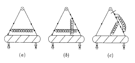
Figure 5: One-loop radiative corrections for two-particle correlators in the Abelian gauge theory. The fermion propagator crossed with a bar on diagram (c) shows the contraction of the corresponding line into the point.

In the calculations of the corresponding evolution kernels, we follow the methods developed in Ref. [9] (see Ref. [21] for a more recent discussion of the RG equations for the time-like twist-3 cut vertices). The one-loop Feynman diagrams giving rise to the transition amplitudes of two-particle correlation functions into the two- and three-parton ones are shown in Fig. 5a, b. The last figure (c) on this picture is specific of the vertices having non-quasi-partonic form [10], that is for $e(x)$ and $h_{L}(x)$; it displays the addendum due to the contact term that results from the cancellation of the propagator adjacent to the quark–gluon and bare vertices. As an output the vertex acquires the three-particle piece. The radiative correction to the three-parton correlators are presented in Fig. 1 a, b, c.

A straightforward calculation yields the evolution equations for the spin-independent case in the form

$$\dot{M}(x) = -\frac{\alpha}{2\pi}\int d\beta M(\beta)\left\{2\left[\frac{\beta}{(x-\beta)}\Theta_{11}^{0}(x,x-\beta)\right]_{+}+\frac{\beta+x}{\beta}\Theta_{11}^{0}(x,x-\beta)\right\},$$ (B.1)

$$\dot{e}(x) = \frac{\alpha}{2\pi}\int d\beta\Biggl{(}e(\beta)\left\{\frac{x}{\beta}\Theta_{11}^{0}(x,x-\beta)+\frac{1}{2}\delta(\beta-x)\right\}$$ (B.2)

$$- M(\beta)\left\{2\left[\frac{\beta}{(x-\beta)}\Theta_{11}^{0}(x,x-\beta)\right]_{+}+x\Theta_{21}^{1}(x,x-\beta)+2\Theta_{11}^{0}(x,x-\beta)\right\}$$

$$- \int d\beta^{\prime}D(\beta,\beta^{\prime})\Biggl{\{}2\left[\frac{\beta}{(x-\beta)}\Theta_{11}^{0}(x,x-\beta)\right]_{+}+\frac{x}{x-\beta}\Theta_{111}^{0}(x,x-\beta,x-\beta+\beta^{\prime})$$

$$+ \delta(\beta-x)\int d\beta^{\prime\prime}\frac{\beta}{\beta^{\prime\prime}}\Theta_{111}^{0}(\beta^{\prime\prime},\beta^{\prime\prime}-\beta,\beta^{\prime\prime}-\beta^{\prime})+2\Theta_{11}^{0}(x,x-\beta)\Biggr{\}}\Biggr{)},$$

$$\dot{D}(x,x^{\prime}) = -\frac{\alpha}{2\pi}\Biggl{\{}\left[\frac{x^{\prime}}{x}e(x)-M(x)\right]\Theta_{11}^{0}(x^{\prime},x^{\prime}-x)-\left[\frac{x}{x^{\prime}}e(x^{\prime})-M(x^{\prime})\right]\Theta_{11}^{0}(x,x-x^{\prime})$$ (B.3)

$$+ \int d\beta^{\prime}\Biggl{(}D(x,\beta^{\prime})\frac{(\beta^{\prime}-x+x^{\prime})}{(x-x^{\prime})}\Theta_{111}^{0}(x^{\prime},x^{\prime}-x,x^{\prime}-x+\beta^{\prime})$$

$$+ \frac{x^{\prime}}{x^{\prime}-\beta^{\prime}}[D(x-x^{\prime}+\beta^{\prime},\beta^{\prime})-D(x,x^{\prime})]\Theta_{11}^{0}(x^{\prime},x^{\prime}-\beta^{\prime})\Biggr{)}$$

$$+ \int d\beta\Biggl{(}D(\beta,x^{\prime})\frac{(\beta-x^{\prime}+x)}{(x^{\prime}-x)}\Theta_{111}^{0}(x,x-x^{\prime},x-x^{\prime}+\beta)$$

$$+ \frac{x}{x-\beta}[D(\beta,x^{\prime}-x+\beta)-D(x,x^{\prime})]\Theta_{11}^{0}(x,x-\beta)\Biggr{)}-\frac{3}{2}D(x,x^{\prime})\Biggr{\}},$$

where the dot denotes the derivative with respect to the UV cutoff $\hskip 2.84544pt\dot{}=\Lambda^{2}{\partial}/{\partial\Lambda^{2}}$ and the plus-prescription is defined by the equation

$$\left[\frac{\beta}{(x-\beta)}\Theta_{11}^{0}(x,x-\beta)\right]_{+}=\frac{\beta}{(x-\beta)}\Theta_{11}^{0}(x,x-\beta)-\delta(\beta-x)\int d\beta^{\prime\prime}\frac{\beta}{(\beta^{\prime\prime}-\beta)}\Theta_{11}^{0}(\beta^{\prime\prime},\beta^{\prime\prime}-\beta).$$ (B.4)

In the same way we can immediately obtain the set of evolution equations for the spin-dependent distributions (20)–(25):

$$\dot{\widetilde{M}}(x) = -\frac{\alpha}{2\pi}\int d\beta\widetilde{M}(\beta)\left\{2\left[\frac{\beta}{(x-\beta)}\Theta_{11}^{0}(x,x-\beta)\right]_{+}+\frac{\beta+x}{\beta}\Theta_{11}^{0}(x,x-\beta)\right\},$$ (B.5)

$$\dot{h}_{1}(x) = -\frac{\alpha}{2\pi}\int d\beta h_{1}(\beta)\left\{2\left[\frac{\beta}{(x-\beta)}\Theta_{11}^{0}(x,x-\beta)\right]_{+}+2\Theta_{11}^{0}(x,x-\beta)-\frac{3}{2}\delta(x-\beta)\right\}\!,$$

$$\dot{h}_{L}(x) = \frac{\alpha}{2\pi}\int d\beta\Biggl{(}h_{L}(\beta)\left\{\frac{x}{\beta}\Theta_{11}^{0}(x,x-\beta)+\frac{1}{2}\delta(\beta-x)\right\}$$ (B.7)

$$- \widetilde{M}(\beta)\left\{2\left[\frac{\beta}{(x-\beta)}\Theta_{11}^{0}(x,x-\beta)\right]_{+}+\left(2+\frac{x}{\beta}\right)\Theta_{11}^{0}(x,x-\beta)\right\}$$

$$- K(\beta)\left\{2\left[\frac{\beta}{(x-\beta)}\Theta_{11}^{0}(x,x-\beta)\right]_{+}+\left(2+3\frac{x}{\beta}\right)\Theta_{11}^{0}(x,x-\beta)-\delta(x-\beta)\right\}$$

$$- \int d\beta^{\prime}\widetilde{D}(\beta,\beta^{\prime})\Biggl{\{}2\left[\frac{\beta}{(x-\beta)}\Theta_{11}^{0}(x,x-\beta)\right]_{+}+\frac{x}{x-\beta}\Theta_{111}^{0}(x,x-\beta,x-\beta+\beta^{\prime})$$

$$+ \delta(\beta-x)\int d\beta^{\prime\prime}\frac{\beta}{\beta^{\prime\prime}}\Theta_{111}^{0}(\beta^{\prime\prime},\beta^{\prime\prime}-\beta,\beta^{\prime\prime}-\beta^{\prime})+2\left(1+\frac{x}{\beta}\right)\Theta_{11}^{0}(x,x-\beta)\Biggr{\}}\Biggr{)},$$

$$\dot{K}(x) = \frac{\alpha}{2\pi}\int d\beta\Biggl{(}2h_{L}(\beta)\frac{x}{\beta}\Theta_{11}^{0}(x,x-\beta)-2\widetilde{M}(\beta)\Theta_{11}^{0}(x,x-\beta)$$

$$- K(\beta)\left\{2\left[\frac{\beta}{(x-\beta)}\Theta_{11}^{0}(x,x-\beta)\right]_{+}+2\left(1+2\frac{x}{\beta}\right)\Theta_{11}^{0}(x,x-\beta)-\frac{3}{2}\delta(x-\beta)\right\}$$

$$- \int d\beta^{\prime}\widetilde{D}(\beta,\beta^{\prime})\Biggl{\{}2\frac{(x-\beta+\beta^{\prime})}{(x-\beta)}\Theta_{111}^{0}(x,x-\beta,x-\beta+\beta^{\prime})+2\frac{x}{\beta}\Theta_{11}^{0}(x,x-\beta)\Biggr{\}}\Biggr{)},$$

$$\dot{\widetilde{D}}(x,x^{\prime}) = -\frac{\alpha}{2\pi}\Biggl{\{}\left[\frac{x^{\prime}}{x}[h_{L}(x)-K(x)]-\widetilde{M}(x)\right]\Theta_{11}^{0}(x^{\prime},x^{\prime}-x)$$ (B.9)

$$+ \left[\frac{x}{x^{\prime}}[h_{L}(x^{\prime})-K(x^{\prime})]-\widetilde{M}(x^{\prime})\right]\Theta_{11}^{0}(x,x-x^{\prime})$$

$$+ \int d\beta^{\prime}\Biggl{(}\widetilde{D}(x,\beta^{\prime})\frac{(\beta^{\prime}-x+x^{\prime})}{(x-x^{\prime})}\Theta_{111}^{0}(x^{\prime},x^{\prime}-x,x^{\prime}-x+\beta^{\prime})$$

$$+ \frac{x^{\prime}}{x^{\prime}-\beta^{\prime}}[\widetilde{D}(x-x^{\prime}+\beta^{\prime},\beta^{\prime})-\widetilde{D}(x,x^{\prime})]\Theta_{11}^{0}(x^{\prime},x^{\prime}-\beta^{\prime})\Biggr{)}$$

$$+ \int d\beta\Biggl{(}\widetilde{D}(\beta,x^{\prime})\frac{(\beta-x^{\prime}+x)}{(x^{\prime}-x)}\Theta_{111}^{0}(x,x-x^{\prime},x-x^{\prime}+\beta)$$

$$+ \frac{x}{x-\beta}[\widetilde{D}(\beta,x^{\prime}-x+\beta)-\widetilde{D}(x,x^{\prime})]\Theta_{11}^{0}(x,x-\beta)\Biggr{)}-\frac{3}{2}\widetilde{D}(x,x^{\prime})\Biggr{\}}.$$

The anomalous dimensions calculated from the evolution equation for the distribution $h_{1}(x)$ coincide (up to the colour group factor $C_{F}$) with the result of Ref. [22].

By exploiting the relation provided by the equation of motion and Lorentz invariance, we can easily verify that the RG equations thus constructed are indeed correct and the renormalization program can be reduced to the study of logarithmic divergences of the three-parton ($Z(x,x^{\prime})$, $\widetilde{Z}(x,x^{\prime})$) and quark mass ($M(x)$, $\widetilde{M}(x)$) correlators in perturbation theory.

Appendix C Local anomalous dimensions

In this appendix we pass from the evolution equations for correlators to the equations for their moments and, in this way, the anomalous-dimension matrix for local twist-3 operators.

We define the moments as follows:

$$F_{n} = \int dxx^{n}F(x)\hskip 14.22636pt\mbox{for any two-particle correlator,}$$

$$Z_{n}^{l} = \int dxdx^{\prime}x^{n-l}x^{\prime l-1}Z(x,x^{\prime}).$$ (C.1)

In the language of operator product expansion these equalities specify the expansion of non-local string operators in towers of local ones, namely:

$${\cal Z}_{n}^{l} = i^{n-1}(-1)^{l-1}\frac{\partial^{l-1}}{\partial\mu^{l-1}}\frac{\partial^{n-l}}{\partial\lambda^{n-l}}\left.{\cal Z}(\lambda,\mu)\right|_{\lambda=\mu=0}$$ (C.4)

$$\hskip 142.26378pt=\frac{1}{2}\bar{\psi}(0)(iD_{+})^{l-1}{\rm g}G_{+\rho}(0)\sigma^{\perp}_{\rho+}\!\left(\!\begin{array}[]{c}I\\ \gamma_{5}\end{array}\!\right)(iD_{+})^{n-l}\psi(0),$$

$${\cal M}_{n} = i^{n}\frac{\partial^{n}}{\partial\lambda^{n}}\,\left.{\cal M}(\lambda)\right|_{\lambda=0}=\frac{m}{2}\bar{\psi}(0)\gamma_{+}\!\left(\!\begin{array}[]{c}I\\ \gamma_{5}\end{array}\!\right)(iD_{+})^{n}\psi(0).$$ (C.7)

The inverse transformations to the non-local representation are given by

$${\cal Z}(\lambda,\mu)=\sum_{n=0,\,m=0}^{\infty}(-i)^{n+m}(-1)^{m}\frac{\mu^{m}}{m!}\frac{\lambda^{n}}{n!}\,{\cal Z}_{n+m+1}^{m+1},\qquad{\cal M}(\lambda)=\sum_{n=0}^{\infty}(-i)^{n}{\lambda^{n}\over n!}\,{\cal M}_{n}.$$ (C.8)

Now it is a simple task to derive the algebraic equations for the mixing of local operators under the change of the renormalization scale from the evolution equations (35)–(39). They are

$$\dot{M}_{n} = \frac{\alpha}{2\pi}{{}_{\scriptscriptstyle MM}\gamma}^{n}M_{n},$$ (C.9)

$$\dot{Z}^{l}_{n} = \frac{\alpha}{2\pi}\left\{\left[{{}_{\scriptscriptstyle ZM}\gamma}^{n}_{n-l+1}\pm{{}_{\scriptscriptstyle ZM}\gamma}^{n}_{l}\right]M_{n}+\sum_{k=1}^{n}{{}_{\scriptscriptstyle ZZ}\gamma}^{n}_{lk}Z_{n}^{k}\right\},$$ (C.10)

where the anomalous dimensions are given by the expressions

$${{}_{\scriptscriptstyle MM}\gamma}^{n} = -C_{F}\left(S_{n}+S_{n+2}\right),$$ (C.11)

$${{}_{\scriptscriptstyle ZM}\gamma}^{n}_{l} = \frac{2C_{F}}{l(l+1)(l+2)},$$ (C.12)

$${{}_{\scriptscriptstyle ZZ}\gamma}^{n}_{lk} = \frac{3}{4}C_{F}\delta(l-k)+\frac{C_{A}}{2}\left\{\theta(l-k-1)\frac{(k+1)(k+2)}{(l-k)(l+1)(l+2)}-\delta(l-k)\left[S_{k-1}+S_{k+2}\right]\right\}$$ (C.13)

$$+ \left(C_{F}-\frac{C_{A}}{2}\right)\biggl{\{}\theta(l-k-1)\left[\frac{2(-1)^{k}C_{l}^{k}}{l(l+1)(l+2)}+\frac{(-1)^{l-k}}{(l-k)}\frac{C_{n}^{k-1}}{C_{n}^{l-1}}\right]$$

$$+ \delta(l-k)\left[\frac{2(-1)^{k}}{k(k+1)(k+2)}-S_{k}\right]\biggr{\}}+{k\rightarrow n-k+1\choose l\rightarrow n-l+1}.$$

Here we have used the following step functions

$$\theta(i-j)=\left\{\begin{array}[]{c}1,\ i\geq j\\ 0,\ i<j\end{array}\right.,\hskip 28.45274pt\delta(i-j)=\left\{\begin{array}[]{c}1,\ i=j\\ 0,\ i\neq j\end{array}\right.,$$ (C.14)

as well as the convention $S_{n}=\sum_{k=1}^{n}\frac{1}{k}$ and the binomial coefficients $C_{n}^{m}=\frac{n!}{m!(n-m)!}$. The plus and minus signs in this equation correspond to the functions $e$ and $h_{L}$, respectively. These analytical expressions coincide with the result of Ref. [15].

         

Figure 2: The spectrum of the eigenvalues $\lambda^{n}_{l}$ for the evolution kernel $P^{n}_{\scriptscriptstyle\cal ZZ}$ defined in (4) is shown in (a). In (b) the relative deviation $1-\lambda^{n}_{l}/(-\gamma^{n}_{l})$ (in %) for the lowest two eigenvalues of the spectrum, i.e. $l=1,2$, is plotted: the solid (dashed) line $\gamma_{n}^{1}$ ($\gamma_{n}^{2}$) corresponds to the $n$-th moments of the improved kernel $P_{ee}$ ($P_{\bar{h}\bar{h}}$) defined by Eq. (5.2); the dash-dotted (dotted) line is the multicolour approximation for $P_{ee}$ ($P_{\bar{h}\bar{h}}$). In the improved approximations, subleading terms were taken into account to reproduce the first two eigenvalues exactly. Eigenfunctions of the kernel $P^{n}_{\cal ZZ}$ are shown for $n=4$ in (c) and for $n=30$ with $l=2,3,6,29$ in (d).

Figure 3: The predictions of the improved evolution equation for the moments $[e]_{n}$, normalized to 1 at $Q_{0}^{2}=1\mbox{\ }{\rm GeV}^{2}$, are shown in (a) for $n=1$ (solid line), $n=2$ (dashed line), $n=10$ (dash-dotted line) and $n=100$ (dotted line). In (b) three different models for the gluon light-cone position distributions at $Q_{0}^{2}=1\mbox{\ }\rm{GeV}^{2}$ for $n=10$ are presented; they are evolved up to the scale $Q^{2}=100\mbox{\ }{\rm GeV}^{2}$ in (c). The relative deviation $1-[e(Q^{2})]_{n}^{\rm ex}/[e(Q^{2})]_{n}^{\rm im}$ (in %) from the improved DGLAP equation of the exact evolution for the assumed gluon distributions is shown in (d). The dotted line corresponds to the relative deviation $1-[e(Q^{2})]_{n}^{N_{c}}/[e(Q^{2})]_{n}^{\rm coef}$ with respect to the multicolour approximation, where “coef” refers to the gluon distribution that is equivalent to the corresponding coefficient function.

Figure 4: The predictions of the improved evolution equation for the moments $[\widetilde{h}_{L}]_{n}$, normalized to 1 at $Q_{0}^{2}=1\mbox{}\rm{GeV}^{2}$, are shown in (a). Here the solid line and dashed line represent $n=2$ and $n=3$, respectively. The further description is the same as in Fig. 3, except that $n=20$ in (b)–(d).

References

• [1] A.H. Mueller, ed., Perturbative Quantum Chromodynamics (World Scientific, Singapore, 1989);
J. Qui and G. Sterman, Nucl. Phys. B 353 (1991) 105; ibid. B 353 (1991) 137.
• [2] J.C. Collins and D.E. Soper, Nucl. Phys. B 194 (1982) 445.
• [3] V.M. Braun, P. Gornicki and L. Mankiewicz, Phys. Rev. D 51 (1995) 6036;
A.V. Belitsky, Phys. Lett. B 386 (1996) 359.
• [4] R.L. Jaffe, Comments Nucl. Part. Phys. 19 (1990) 239.
• [5] R.L. Jaffe and X. Ji, Phys. Rev. Lett. 67 (1991) 552;
R.L. Jaffe and X. Ji, Nucl. Phys. B 375 (1992) 527.
• [6] K. Abe et al., Phys. Rev. Lett. 76 (1996) 587.
• [7] V.N. Gribov and L.N. Lipatov, Sov. J. Nucl. Phys. 15 (1972) 438;
L.N. Lipatov, Sov. J. Nucl. Phys. 20 (1974) 94;
A.P. Bukhvostov, L.N. Lipatov and N.P. Popov, Sov. J. Nucl. Phys. 20 (1974) 287.
• [8] G. Altarelli and G. Parisi, Nucl. Phys. B 126 (1977) 298.
• [9] A.P. Bukhvostov, E.A. Kuraev and L.N. Lipatov, Sov. J. Nucl. Phys. 38 (1983) 263; ibid. 39 (1984) 121;
A.P. Bukhvostov, E.A. Kuraev and L.N. Lipatov, JETP Lett. 37 (1983) 482; Sov. Phys. JETP 60 (1984) 22.
• [10] A.P. Bukhvostov, G.V. Frolov, L.N. Lipatov and E.A. Kuraev, Nucl. Phys. B 258 (1985) 601.
• [11] I.I. Balitsky and V.M. Braun, Nucl. Phys. B 311 (1988/89) 541.
• [12] P.G. Ratcliff, Nucl. Phys. B 264 (1986) 493;
X. Ji and C. Chou, Phys. Rev. D 42 (1990) 3637;
J. Kodaira, Y. Yasui, K. Tanaka and T. Uemastu, Phys. Lett. B 387 (1996) 855.
• [13] B. Geyer, D. MΓΌller and D. Robaschik, Nucl. Phys. Proc. Suppl. 51C (1996) 106;
B. Geyer, D. MΓΌller and D. Robaschik, The evolution of the nonsinglet twist-3 parton distribution function, hep-ph/9611452;
D. MΓΌller, Calculation of higher-twist evolution kernels for polarized deep inelastic scattering, CERN-TH/97-4, hep-ph/9701338.
• [14] A. Ali, V.M. Braun and G. Hiller, Phys. Lett. B 266 (1991) 117.
• [15] Y. Koike and K. Tanaka, Phys. Rev. D 51 (1995) 6125;
Y. Koike and N. Nishiyama, Phys. Rev. D55 (1997) 3068.
• [16] I. Balitsky, V. Braun, Y. Koike and K. Tanaka, Phys. Rev. Lett. 77 (1996) 3078.
• [17] D. MΓΌller, D. Robaschik, B. Geyer, F. M. Dittes and J. HoΕ™ejΕ‘i, Fortschr. Phys. 42 (1994) 101.
• [18] J. Kogut and D.E. Soper, Phys. Rev. D1 (1970) 2901.
• [19] R.L. Jaffe, Nucl. Phys. B 229 (1983) 205.
• [20] For a review, see G. Leibbrandt, Rev. Mod. Phys. 59 (1987) 1067;
A. Bassetto, G. Nardelli and R. Soldati, Yang-Mills theories in the algebraic non covariant gauges (World Scientific, Singapore, 1991).
• [21] A.V. Belitsky and E.A. Kuraev, Evolution of the chiral-odd spin-independent fracture functions in Quantum Chromodynamics, hep-ph/9612256.
• [22] X. Artru and M. Mekhfi, Z. Phys. C 45 (1990) 669.
Β Β Β Β Β Β Β Β Β  Refer to caption