HEP-PH/9702353

Penguin corrections and strong phases in a time-dependent analysis of $\overline{B^{0}}(B^{0})\to{\pi^{+}}{\pi^{-}}$

P. S. Marrocchesi

(Modena University and INFN/Pisa)

N. Paver

(Trieste University and INFN/Trieste)

From a time-dependent analysis of the decay $\stackrel{{\scriptstyle{\scriptscriptstyle(-)}}}{{B^{\scriptscriptstyle 0}_{\scriptscriptstyle d}}}\to{\pi^{+}}{\pi^{-}}$ and using a model-dependent ${A_{\scriptscriptstyle P}}/{A_{\scriptscriptstyle T}}$ ratio of the penguin-to-tree amplitudes contributing to the decay, both the weak phase $\alpha$ and the strong phase shift difference $\delta$ can be extracted from the data. The value of the weak phase $\beta$, expected to be measured from the decay ${B^{\scriptscriptstyle 0}_{\scriptscriptstyle d}}\to J/\psi K^{\scriptscriptstyle 0}_{S}$, is used to parameterize the value of ${A_{\scriptscriptstyle P}}/{A_{\scriptscriptstyle T}}$ and the corresponding penguin correction to the observed asymmetry in ${B^{\scriptscriptstyle 0}_{\scriptscriptstyle d}}\to{\pi^{+}}{\pi^{-}}\/$.

1 Introduction

Measurements of CP violation in $\stackrel{{\scriptstyle{\scriptscriptstyle(-)}}}{{B^{\scriptscriptstyle 0}_{\scriptscriptstyle d}}}\to{\pi^{+}}{\pi^{-}}$ and $\stackrel{{\scriptstyle{\footnotesize(-)}}}{{B^{\scriptscriptstyle 0}_{\scriptscriptstyle d}}}\to J/\psi K^{\scriptscriptstyle 0}_{S}$ decays are expected to provide information, respectively, on the angles $\alpha$ and $\beta$ of the unitarity triangle [1]. As it is well known, in ${B^{\scriptscriptstyle 0}_{\scriptscriptstyle d}}\to J/\psi K^{\scriptscriptstyle 0}_{S}$ the weak phase of the penguin contribution is the same as in the (largely) dominant tree amplitude and therefore the value of $\sin 2\beta\>$ can be directly extracted from the measurement of the time-dependent CP asymmetry with no hadronic uncertainties. In particular, as being dominated by a single amplitude, this channel should be insensitive to the presence of phases of strong-interaction origin.

On the other hand, the extraction of $\sin 2\alpha$ from a time-dependent analysis of the asymmetry in ${B^{\scriptscriptstyle 0}_{\scriptscriptstyle d}}\to{\pi^{+}}{\pi^{-}}\/$ appears to be less straightforward [2]. This is mainly due to the presence of gluonic and electroweak penguin terms with weak phases different from those of the dominant tree $b\to ud\overline{u}$ amplitude. The common prejudice is that the penguin should be smaller than the tree diagram. However, for a quantitatively meaningful statement, the relative size must be either estimated theoretically or measured experimentally from a suitable data sample of $B$-decays. An additional source of uncertainty is introduced by strong-interaction phases which can be different for tree and penguin amplitudes and difficult to model at the non-perturbative hadronic level.

While the size of the tree and penguin amplitudes (in particular, their ratio) can be somehow assessed under some theoretical assumptions, e.g., the factorization hypothesis for non-leptonic decay amplitudes [3], the effect of the strong-interaction phases is much harder to estimate reliably [4]. The conventional expectation is that such phases should not be large. This seems verified by the phases of perturbative origin [5],[6], coming from the $c\bar{c}$ penguin with on-shell $c\bar{c}$ quarks [7, 8], and is expected to be true also for the final state, long distance, non-perturbative phases, considering the high velocity of the produced ${\pi^{+}}{\pi^{-}}\/$ pair. Nevertheless, from considerations based on Regge phenomenology, it has been recently suggested that, contrary to expectations, final state interactions might be important even in B non leptonic decays [9]. Also, significant effects have been estimated by semiquantitative (and model-dependent) calculations for the color suppressed channels $B^{0}\to D^{0}\pi^{0}$ and $B^{0}\to\pi^{0}\pi^{0}$ [10, 11].

Several strategies have been proposed to extract the value of $\sin 2\alpha$ in a model-independent way avoiding the difficulty associated with penguins in ${B^{\scriptscriptstyle 0}_{\scriptscriptstyle d}}\to{\pi^{+}}{\pi^{-}}\/$. However, although quite effective in principle, their application to a practical analysis of the data might run into some difficulties and the effective potential of these methods have still to be realistically assessed by taking into account the expected statistics and experimental sensitivities. For example, the isospin analysis of ${B^{\scriptscriptstyle 0}_{\scriptscriptstyle d}}\to\pi\pi\/$ decays [12], [13],[14] which would enable to directly reconstruct the unitarity triangle, suffers from the predicted low rate for ${B^{\scriptscriptstyle 0}_{\scriptscriptstyle d}}\to\pi^{\scriptscriptstyle 0}\pi^{\scriptscriptstyle 0}\/$, of the order of $10^{-6}$ or less [15, 16], and unfavourable background conditions. Alternative methods require more complicated analyses to fit penguin amplitudes by combining measurements of ${B^{\scriptscriptstyle 0}_{\scriptscriptstyle d}}\to{\pi^{+}}{\pi^{-}}\/$ with different penguin-dominated processes such as $B\to K\pi$ [17, 18, 19, 20, 21, 22] or ${B^{\scriptscriptstyle 0}_{\scriptscriptstyle d}}\to K^{\scriptscriptstyle 0}\overline{K^{\scriptscriptstyle 0}}\/$ [23] and relying on SU(3) symmetry of matrix elements and/or first-order SU(3) breaking. In that case, the sensitivity to $\alpha$ could be rather difficult to fully establish in practice.

The hadronic uncertainty in the extraction of $\sin 2\alpha$ from the CP asymmetry in $\stackrel{{\scriptstyle{\scriptscriptstyle(-)}}}{{B^{\scriptscriptstyle 0}_{\scriptscriptstyle d}}}\to{\pi^{+}}{\pi^{-}}$ has been discussed by many authors and the analysis of this channel extended to other, non-strange, $\Delta S=0$ final states such as $\rho\pi$ or $\rho\rho$, and the corresponding $\Delta S=1$ decays [5, 24, 25, 26, 27]. To derive quantitative results, assumptions are made on the relevant hadronic matrix elements (in general, the factorization model), and on the final state strong interaction effects which in most cases are assumed to be negligible .

In the following, we focus on the determination of $\sin 2\alpha$ from the measured CP time asymmetry in $\stackrel{{\scriptstyle{\scriptscriptstyle(-)}}}{{B^{\scriptscriptstyle 0}_{\scriptscriptstyle d}}}\to{\pi^{+}}{\pi^{-}}$. A discussion of the penguin-induced correction $\Delta\alpha$ in terms of $\alpha$ itself and of the strong phase $\delta=\mbox{${\delta_{\scriptscriptstyle T}}$}-\mbox{${\delta_{\scriptscriptstyle P}}$}$ between tree and penguin amplitudes was presented in [2], where a first-order expansion of the asymmetry in the penguin-to-tree amplitude ratio ${A_{\scriptscriptstyle P}}/{A_{\scriptscriptstyle T}}$ was used. As a result of this analysis, it turns out that $\Delta\alpha$ might be significant, except for large values of the asymmetry and that, in any case, the correction should be maximal for $\delta=0$.

The strong phase effect on $\Delta\alpha$ for general values of $\delta$ has been further considered in [5] using the exact expressions for the CP asymmetry and the tree-to-penguin amplitude ratio from the factorization model as input. The indication from [5] is that, within the assumed model, the expected relative shift in $\alpha$ should not exceed $30\%$ and, similarly to [2], is maximal for $\delta=0$.

In this note, we take a somewhat different point of view and try to gain insight into the actual value of the strong phases difference $\delta$, without a priori assumptions on their size, assuming that both the mixing-induced and the direct CP violation terms will be measured from the time-dependent CP asymmetry of $\stackrel{{\scriptstyle{\scriptscriptstyle(-)}}}{{B^{\scriptscriptstyle 0}_{\scriptscriptstyle d}}}\to{\pi^{+}}{\pi^{-}}$. Similarly to most previous analyses, we assume the approximation where the top mediated penguin dominates (in which case the electroweak phase of the penguin can be identified with the angle $\beta$) and adopt the model dependent estimate of the ratio ${A_{\scriptscriptstyle P}}/{A_{\scriptscriptstyle T}}$ provided by factorization. This ratio then depends on both the “true” value of $\alpha$ and on $\beta$. Using this relation, we evaluate the correction to the “measured” value of $\alpha$ (obtained from the fit of the time-dependent rates in $\stackrel{{\scriptstyle{\scriptscriptstyle(-)}}}{{B^{\scriptscriptstyle 0}_{\scriptscriptstyle d}}}\to{\pi^{+}}{\pi^{-}}$ ), required to determine the “true” value of $\alpha$, as a function of $\beta$ alone. For this correction we use the exact expression for the penguin contribution to the time asymmetry, so that the analysis potentially applies also to the case of large penguin-to-tree amplitude ratio. We also gain information on the effect of the strong phase $\delta$, corresponding to the different possible values of $\beta$. To summarize, from a time-dependent analysis of ${B^{\scriptscriptstyle 0}_{\scriptscriptstyle d}}\to{\pi^{+}}{\pi^{-}}\/$, combined with a clean and accurate independent measurement of the angle $\beta$, we show that one can in principle:

• extract the measured uncorrected value of $\alpha$

• evaluate (a model dependent) correction $\Delta\alpha$

• gain insight into the role played by $\delta$ in $\stackrel{{\scriptstyle{\scriptscriptstyle(-)}}}{{B^{\scriptscriptstyle 0}_{\scriptscriptstyle d}}}\to{\pi^{+}}{\pi^{-}}$.

The price is the introduction of a modest, model-dependent, correlation between two otherwise independent measurements, and the estimate of the ratio ${A_{\scriptscriptstyle P}}/{A_{\scriptscriptstyle T}}$ from factorization.

2 Model-dependent evaluation of ${A_{\scriptscriptstyle P}}/{A_{\scriptscriptstyle T}}$

To make the presentation self-contained, this section briefly reviews the basic points of the derivation of the penguin-to-tree ratio for $\stackrel{{\scriptstyle{\scriptscriptstyle(-)}}}{{B^{\scriptscriptstyle 0}_{\scriptscriptstyle d}}}\to{\pi^{+}}{\pi^{-}}$ in the factorization approach.

The relevant effective weak Hamiltonian can be parameterized as [29, 30, 31]:

$$H_{W}^{eff}=\frac{4G_{F}}{\sqrt{2}}\left[V_{ub}V_{ud}^{*}\left(c_{1}O_{1}+c_{2}O_{2}\right)-V_{tb}V_{td}^{*}\sum_{i}c_{i}O_{i}\right]+h.c.,$$ (1)

where $c_{i}$ are short-distance Wilson coefficients defined at a scale $\mu$ of the order of the heavy quark mass $m_{b}$, and $O_{i}$ are a set of local quark operators with the appropriate quantum numbers. The first two terms in (1) represent the tree diagrams while the other ones are the contributions of strong and electroweak penguin diagrams. For simplicity we can neglect electroweak penguins, which are found to give a small contribution to the mode $\stackrel{{\scriptstyle{\scriptscriptstyle(-)}}}{{B^{\scriptscriptstyle 0}_{\scriptscriptstyle d}}}\to{\pi^{+}}{\pi^{-}}$ of interest here [15, 31, 32]. In any case they could be included following the remarks in [26]. Retaining only strong penguin operators, the sum in (1) reduces to $i\leq 6$ and the explicit expressions of the relevant $O_{i}$ are:

$$\begin{array}[]{l}O_{1}={\bar{d}}^{\alpha}\gamma_{\mu}Lu^{\beta}{\bar{u}}^{\beta}\gamma^{\mu}Lb^{\alpha};\\ O_{3}={\bar{d}}\gamma_{\mu}Lb\sum_{q^{\prime}}{\bar{q}}^{\prime}\gamma^{\mu}Lq^{\prime};\\ O_{5}={\bar{d}}\gamma_{\mu}Lb\sum_{q^{\prime}}{\bar{q}}^{\prime}\gamma^{\mu}Rq^{\prime};\end{array}\qquad\qquad\begin{array}[]{l}O_{2}={\bar{d}}\gamma_{\mu}Lu{\bar{u}}\gamma^{\mu}Lb;\\ O_{4}={\bar{d}}^{\alpha}\gamma_{\mu}Lb^{\beta}\sum_{q^{\prime}}{\bar{q}}^{\prime\beta}\gamma^{\mu}Lq^{\prime\alpha};\\ O_{6}={\bar{d}}^{\alpha}\gamma_{\mu}Lb^{\beta}\sum_{q^{\prime}}{\bar{q}}^{\prime\beta}\gamma^{\mu}Rq^{\prime\alpha},\end{array}$$ (2)

where $\alpha,\beta$ are color indices; $L,R=\frac{1}{2}\left(1\mp\gamma_{5}\right)$; and $q^{\prime}$ runs over all quark flavors. For the corresponding Wilson coefficients at the scale $\mu\sim m_{b}=4.8\hskip 2.0ptGeV$ we use the values [31]

$$\begin{array}[]{l}c_{1}=-0.315;\\ c_{4}=-0.0373;\end{array}\qquad\qquad\begin{array}[]{l}c_{2}=1.150;\\ c_{5}=0.0104;\end{array}\qquad\qquad\begin{array}[]{l}c_{3}=0.0174;\\ c_{6}=-0.0459.\end{array}$$ (3)

In the factorization hypothesis, after Fierz reordering the operator $O_{6}$, one directly obtains from (1) and (2)

$$\begin{array}[]{l}\langle\pi^{+}\pi^{-}|H_{W}^{eff}|{\bar{B}}^{0}\rangle=i\frac{G_{F}}{\sqrt{2}}\left[\left(m_{B}^{2}-m_{\pi}^{2}\right)f_{\pi}F_{0}^{B\to\pi}(m_{\pi}^{2})\right]\left\{V_{ub}V_{ud}^{*}\left(\frac{1}{N}c_{1}+c_{2}\right)\right.\\ \\ \left.-V_{tb}V_{td}^{*}\left[\left(\frac{1}{N}c_{3}+c_{4}\right)+\left(\frac{1}{N}c_{5}+c_{6}\right)\frac{2m_{\pi}^{2}}{\left(m_{b}-m_{u}\right)\left(m_{d}+m_{u}\right)}\right]\right\},\end{array}$$ (4)

where $N$ is the number of colors. The following definitions have been used:

$$\langle\pi^{-}|{\bar{d}}\gamma_{\mu}Lu|0\rangle=-\langle\pi^{-}|{\bar{d}}\gamma_{\mu}Ru|0\rangle=\frac{i}{2}f_{\pi}\left(p_{\pi}\right)_{\mu}$$ (5)

with $f_{\pi}=132\hskip 2.0ptMeV$ the pion decay constant, so that from quarks equations of motion

$$\langle\pi^{-}|{\bar{d}}Lu|0\rangle=-\langle\pi^{-}|{\bar{d}}Ru|0\rangle=\frac{i}{2}\frac{m_{\pi}^{2}f_{\pi}}{m_{d}+m_{u}};$$ (6)

and for the ${\bar{B}}^{0}\to\pi^{+}l^{-}\nu_{l}$ matrix elements [33]:

$$\begin{array}[]{l}\langle\pi^{+}|{\bar{u}}\gamma_{\mu}Lb|{\bar{B}}^{0}\rangle=\langle\pi^{+}|{\bar{u}}\gamma_{\mu}Rb|{\bar{B}}^{0}\rangle=\\ \\ \frac{1}{2}\left[\left(p_{B}+p_{\pi}\right)_{\mu}+\frac{m_{B}^{2}-m_{\pi}^{2}}{q^{2}}q_{\mu}\right]F_{1}^{B\to\pi}(q^{2})+\frac{1}{2}\frac{m_{B}^{2}-m_{\pi}^{2}}{q^{2}}q_{\mu}F_{0}^{B\to\pi}(q^{2}),\end{array}$$ (7)

where $q=p_{B}-p_{\pi}$, so that from equations of motion

$$\langle\pi^{+}|{\bar{u}}Lb|{\bar{B}}^{0}\rangle=\langle\pi^{+}|{\bar{u}}Rb|{\bar{B}}^{0}\rangle=\frac{1}{2}\frac{m_{B}^{2}-m_{\pi}^{2}}{m_{b}-m_{u}}F_{0}^{B\to\pi}(q^{2}).$$ (8)

With both the coefficients $c_{i}$ and the matrix elements of $O_{i}$ real, the penguin amplitude in Eq. (4) has the (weak) phase of $V_{tb}V_{td}^{*}$. It is well-known that, by the unitarity of the CKM matrix, the $top$ penguin dominance occurs if the difference between the $c$- and $u$-mediated penguins can be neglected, which is the case for $m_{c}^{2}/m_{b}^{2}\simeq 0$. However, phenomenological estimates indicate the values $m_{c}=1.3-1.5\hskip 2.0ptGeV$ and $m_{b}=4.5-5\hskip 2.0ptGeV$ [34, 35]. Thus, the verification of such approximation is clearly a point deserving further analysis. As a matter of fact, the consistent treatment of both the Wilson coefficients and the matrix elements of operators at next-to-leading order in QCD provides modifications of order $\alpha_{s}$ to the simple structure of Eqs. (3) and (4). In particular it introduces imaginary parts into the coefficients [15, 31] which determine final state strong interactions phases at the perturbative quark level. The actual value of such phase is somewhat parameter-dependent, although generally quite small, so that in the following we will consider the strong interaction phase as a free parameter with a priori arbitrary possible values including (but in principle not coinciding with) the perturbative effects.

The general decomposition of the decay amplitude for $\stackrel{{\scriptstyle{\scriptscriptstyle(-)}}}{{B^{\scriptscriptstyle 0}_{\scriptscriptstyle d}}}\to{\pi^{+}}{\pi^{-}}$ in terms of tree plus penguin contributions reads:

$$A = A(B^{0}\to\pi^{+}\pi^{-})=A_{T}\>e^{\>i(\delta_{T}+\phi_{T})}+A_{P}\>e^{\>i(\delta_{P}+\phi_{P})}$$

$${\bar{A}} = A({\bar{B}}^{0}\to\pi^{+}\pi^{-})=A_{T}\>e^{\>i(\delta_{T}-\phi_{T})}+A_{P}\>e^{\>i(\delta_{P}-\phi_{P})},$$ (9)

where $(\phi_{T},\phi_{P})$ and $(\delta_{T},\delta_{P})$ are weak and strong phases, respectively. In the top dominance approximation, (9) can be rewritten as

$$A = |V_{ub}^{*}V_{ud}|\>e^{\>i(\delta_{T}+\gamma)}\>T+|V_{tb}^{*}V_{td}|\>e^{\>i(\delta_{P}-\beta)}P$$

$${\bar{A}} = |V_{ub}V_{ud}^{*}|\>e^{\>i(\delta_{T}-\gamma)}\>T+|V_{tb}V_{td}^{*}|\>e^{\>i(\delta_{P}+\beta)}\>P,$$ (10)

where the CKM entries have been factored from the pure hadronic matrix elements $T$ and $P$. In the leading order Wolfenstein parameterization, the unitarity triangle angles :

$$\alpha=arg\left(-\frac{V_{td}V_{tb}^{*}}{V_{ud}V_{ub}^{*}}\right);\qquad\quad\beta=arg\left(-\frac{V_{cd}V_{cb}^{*}}{V_{td}V_{tb}^{*}}\right);\qquad\quad\gamma=arg\left(-\frac{V_{ud}V_{ub}^{*}}{V_{cd}V_{cb}^{*}}\right)$$ (11)

are related to the parameters $\rho$ and $\eta$ as

$$\tan\alpha=\frac{\eta}{\eta^{2}-\rho\left(1-\rho\right)};\qquad\tan\beta=\frac{\eta}{1-\rho};\qquad\tan\gamma=\frac{\eta}{\rho}.$$ (12)

Comparing (10) to (4) one directly reads the expressions of $T$ and $P$ in the factorization approach:

$$T = \>\>\>\>\>\>\frac{G_{F}}{\sqrt{2}}\left[\left(m_{B}^{2}-m_{\pi}^{2}\right)f_{\pi}F_{0}^{B\to\pi}(m_{\pi}^{2})\right]\left(\frac{1}{N}c_{1}+c_{2}\right),$$ (13)

$$\>\>\>\>\>\>\>P = -\frac{G_{F}}{\sqrt{2}}\left[\left(m_{B}^{2}-m_{\pi}^{2}\right)f_{\pi}F_{0}^{B\to\pi}(m_{\pi}^{2})\right]$$ (14)

$$\times \left[\left(\frac{1}{N}c_{3}+c_{4}\right)+\left(\frac{1}{N}c_{5}+c_{6}\right)\frac{2m_{\pi}^{2}}{\left(m_{b}-m_{u}\right)\left(m_{d}+m_{u}\right)}\right].$$

From (13) and (14) one can notice the property of the ratio $P/T$ of being independent of particular models for the $B\to\pi$ form factors. Thus, apart from the factorization hypothesis itself, it only depends on the short-distance coefficients which can slightly vary according to the choice of the scale $\mu$, and on the current quark masses in the last term of (14). We choose $m_{b}=4.8\hskip 2.0ptGeV$, $m_{d}+m_{u}=15\hskip 2.0ptMeV$ so that, with the coefficients (3) and $N=3$ (the dependence on $N$ is weak), one finds, as in [5, 26], $P/T\simeq 0.055$ . Reasonable variations of quark masses around the chosen values, taking into account the spread of the various determinations, can affect the term mentioned above by about 30%. However, being anyway suppressed in (14) by the large $m_{b}$ and small short distance penguin coefficients, this reflects into an uncertainty on the ratio $P/T$ of the order of 10%.

3 Discussion on the penguin correction $\Delta\alpha$

The time-dependent decay rates are given by :

$$\Gamma(B^{0}(\overline{B^{0}})\to{\pi^{+}}{\pi^{-}})=\frac{\mid\overline{A}\mid^{2}+\mid A\mid^{2}}{2}\>e^{-\Gamma\mid t\mid}\>(1\pm\mbox{$a_{0}\>$\/}\sin{\Delta mt}\pm\mbox{$b_{0}\>$\/}cos{\Delta mt})$$ (15)

where the two real coefficients $a_{0}\>$ and $b_{0}\>$ are :

$$\mbox{}\mbox{$a_{0}\>$\/}=\frac{2\>{\cal I}m\>(e^{2i\beta}A\overline{A}^{*})}{\mid A\mid^{2}+\mid\overline{A}\mid^{2}}$$

(16)

$$\mbox{}\mbox{$b_{0}\>$\/}=\frac{\mid A\mid^{2}-\mid\overline{A}\mid^{2}}{\mid A\mid^{2}+\mid\overline{A}\mid^{2}}$$

In terms of the ratio of the penguin to tree contribution ${A_{\scriptscriptstyle P}}/{A_{\scriptscriptstyle T}}$, the two coefficients $a_{0}\>$ and $b_{0}\>$ can be written as :

$$\mbox{$a_{0}\>$\/}=\frac{-\sin 2\alpha\,+2\>(\mbox{${A_{\scriptscriptstyle P}}/{A_{\scriptscriptstyle T}}$})\cos\delta\>\sin\alpha}{1-2\>(\mbox{${A_{\scriptscriptstyle P}}/{A_{\scriptscriptstyle T}}$})\>\cos\delta\>\cos\alpha+(\mbox{${A_{\scriptscriptstyle P}}/{A_{\scriptscriptstyle T}}$})^{2}}$$ (17)

$$\mbox{$b_{0}\>$\/}=\frac{-2\>(\mbox{${A_{\scriptscriptstyle P}}/{A_{\scriptscriptstyle T}}$})\>\sin\delta\>\sin\alpha}{1-2\>(\mbox{${A_{\scriptscriptstyle P}}/{A_{\scriptscriptstyle T}}$})\>\cos\delta\>\cos\alpha+(\mbox{${A_{\scriptscriptstyle P}}/{A_{\scriptscriptstyle T}}$})^{2}}$$ (18)

where $\delta\equiv\mbox{${\delta_{\scriptscriptstyle T}}$}-\mbox{${\delta_{\scriptscriptstyle P}}$}$ is the strong phases difference and, as in eq.(10), $\>\mbox{${\phi_{\scriptscriptstyle T}}$}-\mbox{${\phi_{\scriptscriptstyle P}}$}=\gamma+\beta=\pi-\alpha$ in the SM. When $\mbox{${A_{\scriptscriptstyle P}}/{A_{\scriptscriptstyle T}}$}=0\>$, the $b_{0}\>$ term vanishes and $\alpha$ is extracted from the simple relation $\mbox{$a_{0}\>$\/}=-\sin 2\alpha\,$. Else, a $\Delta\alpha$ correction term which depends both on $\alpha$ and $\cos\delta$ , has to be added. The $\Delta\alpha$ correction is therefore maximal for $\delta=0$, as pointed out previously.
The ratio of the CKM matrix elements in ${A_{\scriptscriptstyle P}}/{A_{\scriptscriptstyle T}}$ can be expressed in terms of the angles $\alpha$ and $\beta$ of the unitary triangle as :

$$\frac{\mid\mbox{$V_{tb}$}\mbox{$V^{*}_{td}$}\mid}{\mid\mbox{$V_{ub}$}\mbox{$V^{*}_{ud}$}\mid}=\frac{\sin\gamma}{\sin\beta}\>$$ (19)

and therefore, in terms of the ratio of pure hadronic matrix elements $P/T$

$$\frac{\mbox{${A_{\scriptscriptstyle P}}$}}{\mbox{${A_{\scriptscriptstyle T}}$}}=(\sin\alpha\cot\beta+\cos\alpha)\>(\frac{P}{T})$$ (20)

The expected value of the ratio ${A_{\scriptscriptstyle P}}/{A_{\scriptscriptstyle T}}$ — calculated using the $P/T$ value obtained in the previous section — is plotted in fig. 1 as a function of $\alpha$ for four different values of $\beta$.

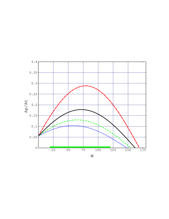
Figure 1: ${A_{\scriptscriptstyle P}}/{A_{\scriptscriptstyle T}}$ plotted against the weak phase $\alpha$ for four different values of $\beta=11^{\circ}$ (dashed upper curve), $18^{\circ}$ (solid), $25^{\circ}$ (dashed), $32^{\circ}(dotted)\>\>\>$.

The curves in fig. 1 are drawn for $\beta=11^{\circ},18^{\circ},25^{\circ},32^{\circ}$, respectively and the highest (lowest) curve lies close to the present experimental lower (upper) limit on $\beta$ [36],[37],[38]. In the same picture, the current experimental bounds on $\alpha$ are superimposed onto the horizontal axis.
From inspection of fig. 1, we would conclude that the value of ${A_{\scriptscriptstyle P}}/{A_{\scriptscriptstyle T}}$ predicted by the model could be as large as 0.3 if the value of $\beta$ would turn out to be close to its present lower limit. However, we must keep in mind that the allowed ranges for $\sin 2\alpha$ and $\sin 2\beta\,$ are correlated through the common dependence on $\rho$ and $\eta$ (see figs. 2(a),(b)). Therefore, the values of $\alpha$ and $\beta$ are allowed to cover a subset of the region bounded in fig. 1 by the envelope of the $\beta$ curves and by the $\alpha$ limits on the ascissa.

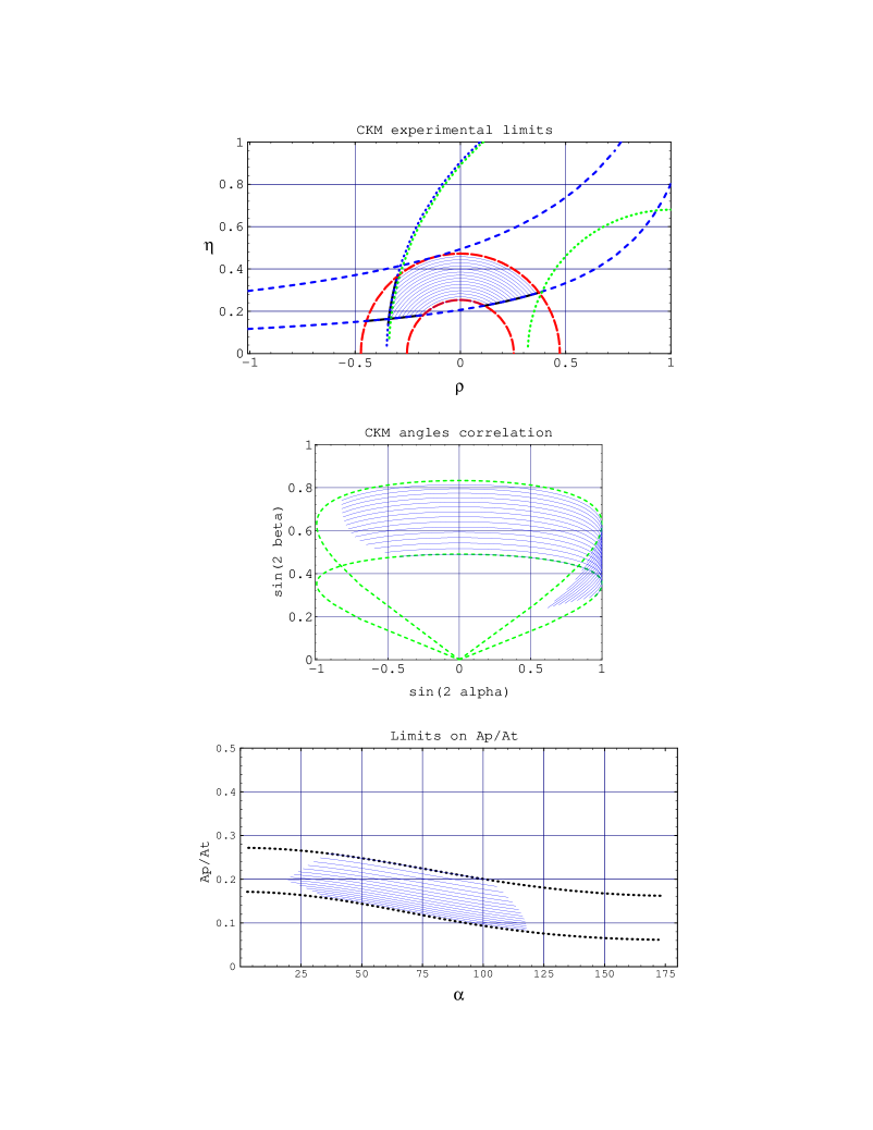
Figure 2: (a) current experimental limits in the ($\rho,\eta$) plane ; (b) correlation between $\sin 2\beta\,$ and $\sin 2\alpha\>$ ; (c) current bounds on ${A_{\scriptscriptstyle P}}/{A_{\scriptscriptstyle T}}$ plotted vs. $\>\alpha$ for $P/T=0.055\>$.

This is best shown in fig. 2(c) where the present limits on the CKM triangle [36],[37],[38] are used to bound the shaded area which represents the allowed value of ${A_{\scriptscriptstyle P}}/{A_{\scriptscriptstyle T}}$ as a function of $\alpha$. From the picture, we see that the penguin to tree amplitude ratio can, at present, vary from a minimum of 0.08 to a maximum of 0.26, approximately.
From equation (17), the correction $\Delta\mbox{$a_{0}\>$\/}$ to the observed value of the $a_{0}\>$ coefficient

$$\Delta\mbox{$a_{0}\>$\/}=\mbox{$a_{0}\>$\/}+\sin 2\alpha$$

is plotted in fig. 3(a) for $\delta=0$, as a function of $\alpha$. For the same value of $\delta$, fig. 3(b) shows the $\Delta\mbox{$a_{0}\>$\/}$ correction obtained, as in [2], by expanding equation (17) to first order in ${A_{\scriptscriptstyle P}}/{A_{\scriptscriptstyle T}}$

$$\Delta\mbox{$a_{0}\>$\/}=-2\>(\mbox{${A_{\scriptscriptstyle P}}/{A_{\scriptscriptstyle T}}$})\>\sin\alpha\>\cos 2\alpha\>\cos\delta$$ (21)

and taking $\delta=0$, while fig. 3(c) shows the difference between the exact and the first order result. A common feature is that the $\Delta\mbox{$a_{0}\>$\/}$ correction is positive in the interval $\pi/4<\alpha<3\pi/4$ while it has the opposite sign and is smaller in magnitude, outside this range. However, while the first order expansion predicts a correction which vanishes for $\alpha=\pi/4$ and $\alpha=3\pi/4$ ( for any value of $\beta$ ) and is maximal for $\alpha=\pi/2$, the second order term introduces a dependence on $\beta$ in the position of the zeroes and of the maximum of the $\Delta\mbox{$a_{0}\>$\/}$ correction. Within the presently allowed range of $\alpha$, the largest difference in $|\Delta\mbox{$a_{0}\>$\/}|$ between the exact $\Delta\mbox{$a_{0}\>$\/}$ correction from eq.(17) and the first order approximation of eq.(21) shows up ( see fig. 3(c)) at $\alpha\approx 60^{\circ}$ and $\alpha\approx 105^{\circ}$ approximately, while it is negligible for $\alpha$ values close to $\pi/2$. It is worth noticing that we have used a positive value for $P/T$ as provided by the model. When reversing its sign, the correction $\Delta\mbox{$a_{0}\>$\/}$ changes sign too.
Rewriting the (second order) expressions for the two parameters $a_{0}\>$ and $b_{0}\>$ in terms of $\alpha$ ,$\>\delta\>$ and ${A_{\scriptscriptstyle P}}/{A_{\scriptscriptstyle T}}$  in eqs.(17) and (18) as :

$$\mbox{$a_{0}\>$\/}+\sin 2\alpha-2\>(\mbox{${A_{\scriptscriptstyle P}}/{A_{\scriptscriptstyle T}}$})\>\cos\delta\>(\>\mbox{$a_{0}\>$\/}\cos\alpha\>+\sin\alpha\>)+\mbox{$a_{0}\>$\/}\>(\mbox{${A_{\scriptscriptstyle P}}/{A_{\scriptscriptstyle T}}$})^{2}=\>0$$ (22)

$$\mbox{$b_{0}\>$\/}-2\>(\mbox{${A_{\scriptscriptstyle P}}/{A_{\scriptscriptstyle T}}$})\>(\>\mbox{$b_{0}\>$\/}\>\cos\delta\>\cos\alpha\>-\sin\delta\>\sin\alpha\>)+\mbox{$b_{0}\>$\/}\>(\mbox{${A_{\scriptscriptstyle P}}/{A_{\scriptscriptstyle T}}$})^{2}=\>0$$ (23)

and inserting ${A_{\scriptscriptstyle P}}/{A_{\scriptscriptstyle T}}$ from (20) into eqs.(22), (23) with the value of $P/T$ provided by the model, we get two equations in the two unknowns $\alpha$ and $\delta$, both a function of the $\beta$ angle : $\alpha=\alpha(\beta)$ and $\delta=\delta(\beta)$ .

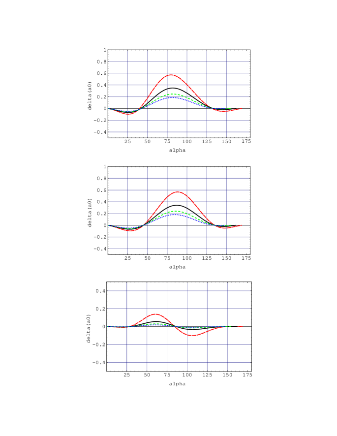
Figure 3: $\Delta\mbox{$a_{0}\>$\/}$ correction plotted against the weak phase $\alpha$ for $\delta=0$ and four different values of $\beta=11^{\circ}$ (dashed upper curve), $18^{\circ}$ (solid), $25^{\circ}$ (dashed), $32^{\circ}(dotted)\>\>\>$ (a) : exact correction ;    (b) : approximate correction to first order in ${A_{\scriptscriptstyle P}}/{A_{\scriptscriptstyle T}}$ ; (c) : difference (a)-(b).

Once $\beta$ is known from an independent measurement ( e.g.: from the decay ${B^{\scriptscriptstyle 0}_{\scriptscriptstyle d}}\to J/\psi K^{\scriptscriptstyle 0}_{S}$ ) and the two parameters $a_{0}\>$ and $b_{0}\>$ are fitted from the $\stackrel{{\scriptstyle{\scriptscriptstyle(-)}}}{{B^{\scriptscriptstyle 0}_{\scriptscriptstyle d}}}\to{\pi^{+}}{\pi^{-}}$ time-dependent decay rates, we can in principle extract the correct value of $\alpha$, from the data, together with a measurement of the relative strong phase $\delta$.

4 Numerical solutions for $\Delta\alpha$ and $\delta$

For a given value of $\beta$, we solve numerically the system of two equations (22) and (23) in the two unknowns $\alpha$ and $\delta$ and find the correction $\Delta\alpha$ to be applied to the measured value ${\alpha_{\scriptscriptstyle M}}$ of $\alpha$ defined as :

$$\Delta\alpha=\mbox{${\alpha_{\scriptscriptstyle M}}$}-\alpha$$

where ${\alpha_{\scriptscriptstyle M}}$ is inferred from the fitted value of the $a_{0}\>$ coefficient, with no penguin corrections, via the relation :

$$-\sin 2\mbox{${\alpha_{\scriptscriptstyle M}}$}=\mbox{$a_{0}\>$\/}$$

Since the value of the measured asymmetry parameter $a_{0}\>$ is related to the weak phase ${\alpha_{\scriptscriptstyle M}}$ via the above circular relation, one cannot distinguish between the case where ${\alpha_{\scriptscriptstyle M}}$ falls into the $[\>45^{\circ},135^{\circ}\>]$ interval or outside. Therefore, for $-1<\mbox{$a_{0}\>$\/}<1\>\>\>$, two numerical solutions for the true value of $\alpha$ are found. The first one corresponds to the above interval for ${\alpha_{\scriptscriptstyle M}}$, while the second solution belongs to the $[\>0^{\circ},45^{\circ}]$ interval for $\mbox{$a_{0}\>$\/}<0$ and to the $[\>135^{\circ},180^{\circ}\>]\>$ interval for $\mbox{$a_{0}\>$\/}>0$ .

Before taking into account the constraints from the present experimental bounds on $\alpha$ and $\beta$, we first examine the predictions for both solutions i.e.: with $\alpha$ spanning the full $[0\>,\>\pi-\beta]$ interval.

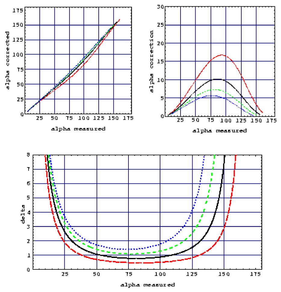
Figure 4: For four different values of $\beta=11^{\circ}$ (dashed), $18^{\circ}$ (solid), $25^{\circ}$ (dashed), $32^{\circ}$ (dotted) and $\>P/T=0.055\>\>$ : (a) “$\alpha$ corrected” vs. “$\alpha$ measured” ; (b) $\Delta\alpha$ correction vs. “$\alpha$ measured”; (c) relative strong phase $\delta$ vs. “$\alpha$ measured” ( see section 4 for a detailed explanation of this picture ).

The penguin correction $\Delta\alpha$

The “penguin-corrected” weak phase $\alpha$ and the correction $\Delta\alpha$ resulting from our analysis are plotted in fig. 4(a) and fig. 4(b), respectively, against the measured ( uncorrected ) value ${\alpha_{\scriptscriptstyle M}}$ in ${B^{\scriptscriptstyle 0}_{\scriptscriptstyle d}}\to{\pi^{+}}{\pi^{-}}\/$ for four different values of $\beta=11^{\circ},18^{\circ},25^{\circ},32^{\circ}$ and with a fixed value of $\mbox{$b_{0}\>$\/}=-5.0\>10^{-3}$. This value has been chosen as an example where the value of the $b_{0}\>$ parameter is very small, but not identically zero, to exemplify a case where $\delta\neq 0$.

From inspection of fig. 4(a) and fig. 4(b) we note that :

• the $\Delta\alpha$ correction increases when $\beta$ decreases. A maximum $\Delta\alpha$ correction of about $16.5^{\circ}$ is found for $\beta=11^{\circ}$. The correction does not exceed $10^{\circ}$ for $\beta$ values greater than $18^{\circ}$, approximately.

• maximal $\Delta\alpha$ corrections for different $\beta$ values occur when ${\alpha_{\scriptscriptstyle M}}$ lies within the approximate interval ($[\>70^{\circ},100^{\circ}]$) and the true value of $\alpha$ corresponding to the maximum of the correction is found to increase when $\beta$ decreases. However, to establish the maximal correction – allowed within the present limits on $\alpha$ and $\beta$ – one should take into account the correlation between the allowed ranges of the two weak phases, as already pointed out for fig. 1.

The “penguin-corrected” value of the asymmetry $-\sin 2\alpha$ in ${B^{\scriptscriptstyle 0}_{\scriptscriptstyle d}}\to{\pi^{+}}{\pi^{-}}\/$, corresponding to ${\alpha_{\scriptscriptstyle M}}$ in the $[\>45^{\circ},135^{\circ}\>]$ interval, is plotted in fig. 5 against the measured value of $a_{0}\>$ for four different values of $\beta=11^{\circ},18^{\circ},25^{\circ},32^{\circ}$ and with $\mbox{$b_{0}\>$\/}=0$. As expected from fig. 3(a) , we note that the measured value of $a_{0}\>$ is significantly higher than the “true” value $-\sin 2\alpha$ and that the correction increases for decreasing $\beta$ values. On the contrary, when ${\alpha_{\scriptscriptstyle M}}$ lies outside the above interval, the correction ( not shown in this picture) to the true value of $\alpha$ is marginal and of opposite sign with respect to the previous case ( i.e.: the measured value of $a_{0}\>$ is slightly larger than the “true” value ).

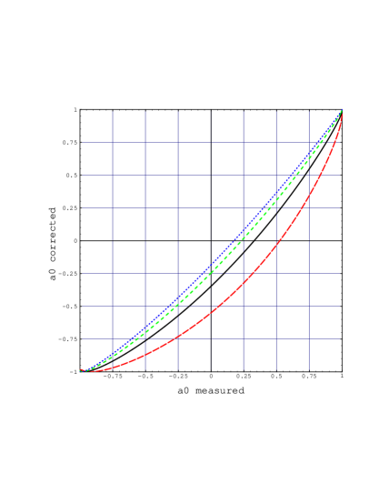
Figure 5: $-\sin 2\alpha$ vs. measured $a_{0}\>$ for four different values of $\beta=11^{\circ}$ (dashed), $18^{\circ}$ (solid), $25^{\circ}$ (dashed), $32^{\circ}(dotted)$ with $\mbox{$b_{0}\>$\/}=0$ and $\>P/T=0.055\>\>\>$.

The strong phases difference $\delta$

In the above example, the values of the solution for the strong phases difference $\delta$ corresponding to a measured value ${\alpha_{\scriptscriptstyle M}}$ are plotted as the family of curves in fig. 4(c) for the same values of $\beta$ used in the previous plots. In the picture, we note that the relative strong phase $\delta$ shows a broad minimum which covers most of the region where $\alpha$ is bounded at present. In our example, the value of the $b_{0}\>$ parameter being very close to zero, the minimum value of $\delta$ turns out to be quite small ($<2^{\circ}\>$, approximately). On the contrary, the value of $\delta$ shows a fast increase when $\alpha$ approaches the two “geometrical” limits 0 or $(\pi-\beta)$. We want to stress that the dependence of $\delta$ on ${\alpha_{\scriptscriptstyle M}}$ in fig. 4(c) has no direct physical meaning. Instead, it describes the parametric behaviour of the solutions of (22) and (23) for the unknowns $\delta$ and $\alpha$ when the value of the $b_{0}\>$ parameter is kept fixed at a non zero value and $a_{0}\>$ is varied. The behaviour of $\delta$ on the ascissa in fig. 4(c) can be understood by considering the following (exact) relation :

$$\tan\delta=\frac{\mbox{$b_{0}\>$\/}[\cos 2\alpha-(\mbox{${A_{\scriptscriptstyle P}}/{A_{\scriptscriptstyle T}}$})^{2}]}{\mbox{$a_{0}\>$\/}[1+(\mbox{${A_{\scriptscriptstyle P}}/{A_{\scriptscriptstyle T}}$})^{2}]+\sin 2\alpha}$$ (24)

which can be easily derived from eqs.(17) and (18).
The ratio ${A_{\scriptscriptstyle P}}/{A_{\scriptscriptstyle T}}$ is found, from eq.(20), to vanish in the limit $\alpha\rightarrow(\pi-\beta)$, while $\mbox{${A_{\scriptscriptstyle P}}/{A_{\scriptscriptstyle T}}$}=P/T=0.055$ for $\alpha=0\>\>$ (see also fig. 1). Correspondingly, $\>\Delta\mbox{$a_{0}\>$\/}\rightarrow 0$ for both $\alpha\rightarrow 0$ and $\alpha\rightarrow(\pi-\beta)$. Therefore, when $\alpha$ is close to zero, the numerator of eq.(24) is almost constant, while the denominator approaches zero since, in this case, the $\Delta\mbox{$a_{0}\>$\/}$ correction is almost negligible and the measured asymmetry $a_{0}\>$ does not differ significantly from the true asymmetry which is identically zero (see fig. 4(b)).
A similar, but not identical behaviour, takes place for $\alpha\rightarrow(\pi-\beta$). This accounts for the fast increase of $\delta$ on the final portion of the curves in fig. 4(c), drawn for the four different values of $\beta$ when $\alpha$ approaches the respective values $\pi-\beta$.

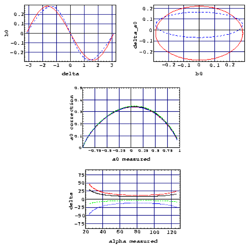
Figure 6: With $\beta=18^{\circ}$ in the four pictures :    (a)  $b_{0}\>$ vs. $\delta\>\>$ and (b) $\>\Delta\mbox{$a_{0}\>$\/}$ vs. $b_{0}\>$   for $\alpha=104.8^{\circ}$ (solid) and $\alpha=56.5^{\circ}$(dashed).   Taking four different values of $\mbox{$b_{0}\>$\/}=-0.075$ (dashed), $-0.050$ (solid), $+0.025$ (dashed), $+0.075$ (dotted) :    (c) correction $\Delta\mbox{$a_{0}\>$\/}$ vs. the measured asymmetry $a_{0}\>$ ; (d) relative strong phase $\delta$ vs. “$\alpha$ measured”.   

4.1 The role of the $b_{0}\>$parameter

The relation between $b_{0}\>$ and $\delta$, for given values of $\alpha$ and $\beta$, is given in eq.(18). Using the value of $P/T$ from section 2, the numerator of (18) is found to dominate over the weak $\cos\delta$ dependence of the denominator and therefore $b_{0}\>$ turns out to be approximately proportional to $-\sin\delta\>$. This dependence is shown in fig. 6(a) where, taking $\beta=18^{\circ}$ and letting $-\pi\leq\delta\leq\pi$, we plot $b_{0}\>$ as a function of $\delta$ for two values of $\alpha=104.8^{\circ}$ (solid line) and $\alpha=56.5^{\circ}$(dashed). In the same figure, the values of $\delta$ corresponding to a minimum or a maximum for $b_{0}\>$ are not too far from $\pm\pi/2$ for both curves in our example, as the absolute value of the $b_{0}\>$ parameter is maximal for $\cos\delta=2(A_{P}/A_{T})\cos\alpha\>/\>[1+(A_{P}/A_{T})^{2}]$.
In order to show the dependence of the “penguin-correction” $\Delta\mbox{$a_{0}\>$\/}$, defined in eq.(3), on the actual value of the $b_{0}\>$ parameter, we stick to the above example and plot $\Delta\mbox{$a_{0}\>$\/}$ as a function of $b_{0}\>$ in fig. 6(b). For $-\pi\leq\delta\leq\pi$ , we found that $\Delta\mbox{$a_{0}\>$\/}$ and $b_{0}\>$ satisfy an elliptic constraint (whose geometrical parameters depend on the choice of $\alpha$ and $\beta$). This is readily verified using the first order expansion (21) in ${A_{\scriptscriptstyle P}}/{A_{\scriptscriptstyle T}}$ of equation (17) and the analogous expansion of (18). In this approximation, the constraint is simply :

$$[\frac{\Delta\mbox{$a_{0}\>$\/}}{2\>(\mbox{${A_{\scriptscriptstyle P}}/{A_{\scriptscriptstyle T}}$})\sin\alpha\>\cos 2\alpha}]^{2}+[\frac{\mbox{$b_{0}\>$\/}}{2\>(\mbox{${A_{\scriptscriptstyle P}}/{A_{\scriptscriptstyle T}}$})\sin\alpha}]^{2}=1$$ (25)

Using instead the (exact) equations (17) and (18) , the constraint is no longer represented by the approximate implicit form (25) and the ellipse is shifted along the $\Delta\mbox{$a_{0}\>$\/}$ axis as in fig. 6(b) by a quantity which depends both on $\alpha$ and $\beta$ (see next paragraph).
The position of a point along the ellipse is parametrized in terms of the relative strong phase $\delta$. For both curves in the example of fig. 6(b), a maximal positive (negative) correction $\Delta\mbox{$a_{0}\>$\/}$ is reached for $\delta=0\>$ ($\delta=\pm\pi\>$) where $\mbox{$b_{0}\>$\/}=0$. For not too large values of $\delta$, which correspond to $|\mbox{$b_{0}\>$\/}|$ values close to zero, the correction $\Delta\mbox{$a_{0}\>$\/}$ is positive and almost independent of $|\mbox{$b_{0}\>$\/}|$. On the contrary, the asymmetry correction $\Delta\mbox{$a_{0}\>$\/}$ decreases rapidly as a function of $|\mbox{$b_{0}\>$\/}|$ ( see fig. 6(b) ) when this parameter approaches its maximum allowed value (for a given $\alpha$ and $\beta$) and the corresponding $\delta$ is close to $\pm\pi/2$. For even larger strong phases, $\>\Delta\mbox{$a_{0}\>$\/}$ may become negative. However, as pointed out previously, large values of $|\mbox{$b_{0}\>$\/}|$ would only occur for unexpectedly large strong phases.
An example where the magnitude of $b_{0}\>$ is kept small is shown in fig. 6(c) where again we keep $\beta=18^{\circ}$ fixed and, using the solutions of (22) and (23), we plot $\Delta\mbox{$a_{0}\>$\/}$ vs. $a_{0}\>$ for four different values of $\>\mbox{$b_{0}\>$\/}=-0.075\>,\>\>\>$ $\>-0.050\>,\>\>\>$ $\>0.025\>,\>\>\>$ $\>0.075\>\>\>\>$. In this range, we find that $\Delta\mbox{$a_{0}\>$\/}$ scales approximately as $\cos\delta$ and therefore $\Delta\mbox{$a_{0}\>$\/}$ is only marginally affected by $b_{0}\>$. In this example, the corresponding solutions for $\delta$ are those of fig. 6(d) where $\delta$ is plotted against the measured angle ${\alpha_{\scriptscriptstyle M}}$ .
In conclusion, the value of the $b_{0}\>$ parameter is found to provide useful information on the strong phases difference $\delta$. If $\delta$ turns out to assume large values ( contrary to the conventional expectation ), then the parameter $b_{0}\>$ is expected to be large in magnitude and to contribute significantly to the assessment of the “penguin corrected” value of $\alpha$, which is otherwise determined by the value of $a_{0}\>$ only.
The current experimentally allowed range for the $b_{0}\>$ parameter is discussed in the following paragraph.

Figure 7: Current bounds from CKM limits on : (a) maximal allowed value of the $b_{0}\>$ parameter plotted against $\alpha$ ; (b) penguin-corrected asymmetry vs. measured asymmetry $a_{0}\>$; (c) strong phase $\delta$ vs. measured asymmetry $a_{0}\>$ for $\mbox{$b_{0}\>$\/}=\pm 0.1$. (d) same as (c) for $\mbox{$b_{0}\>$\/}=\pm 0.05\>$ .

4.2 Bounds from the present CKM limits

The maximum value $|\mbox{${b^{\>max}_{0}}$}|$ allowed by the present experimental CKM limits [36],[37],[38] is plotted in fig. 7(a) as a function of the true value of $\alpha$ when both $\alpha$ and $\beta$ are allowed to vary through their common dependence on $\rho$ and $\eta$ within the domain shown in fig. 2(b).
The values allowed at present by the experimental CKM limits for the “penguin-corrected” asymmetry $-\sin 2\alpha$ are plotted in fig. 7(b) against the measured value of the asymmetry $\mbox{$a_{0}\>$\/}=-2\sin\mbox{${\alpha_{\scriptscriptstyle M}}$}$ by varying $\>-\pi\leq\delta\leq\pi\>$ in such a way to account for all possible allowed values of $b_{0}\>$. As pointed out previously, the measured value of $a_{0}\>$ is significantly higher than the “true” value of the asymmetry when ${\alpha_{\scriptscriptstyle M}}$ belongs to the interval $[\>45^{\circ},135^{\circ}\>]$. On the contrary, we can see in this picture that ${\alpha_{\scriptscriptstyle M}}$ solutions located in the approximate range $[\>20^{\circ},45^{\circ}\>]$ produce a marginal correction to the true value of $\alpha$ of opposite sign with respect to the previous case (i.e.: the measured value of $a_{0}\>$ is slightly smaller than the “true” value ).
Following a different approach, if we keep the magnitude of $|\mbox{$b_{0}\>$\/}|\>$ fixed and let $\alpha$ and $\beta$ vary within the present CKM bounds, we can extract, as a solution of (22) and (23), the value of $\delta$ which corresponds to a given observed value of the asymmetry $a_{0}\>$. This is plotted in fig. 7(c), where we have allowed for our ignorance of the sign of $b_{0}\>$, and we have superimposed on the same picture two examples. The bounded area with positive (negative) values of $\delta$ corresponds to $\mbox{$b_{0}\>$\/}=-0.1$ and $\mbox{$b_{0}\>$\/}=0.1$, respectively. For large negative values of $a_{0}\>$ on the left side of figs. 7(c),(d) two solutions for $\delta$ are found : the one with larger absolute values of $\delta$ again corresponds to the approximate interval $[\>20^{\circ},45^{\circ}\>]$ for ${\alpha_{\scriptscriptstyle M}}$ not (yet) ruled out by the present experimental limits. A similar example is shown in fig. 7(d) for $\mbox{$b_{0}\>$\/}=\pm 0.05$ and where $|\delta|$ is of order $10^{\circ}\>$ over a large fraction of the accessible range of $a_{0}\>$.
Next, we want to establish the combined bounds for the $a_{0}\>$ and $b_{0}\>$ parameters. For a given choice of $\alpha$ and $\beta$, the two parameters $a_{0}\>$ and $b_{0}\>$ are constrained onto one ellipse in the ($a_{0}\>$, $b_{0}\>$) plane and the value of the parameter $\delta$ is used to define the position of the point along the curve. From the (exact) equations (17) and (18), the constraint turns out to be an ellipse displaced along the $a_{0}\>$ axis by the amount $\overline{a_{0}}\>$ :

$$(\frac{\mbox{$a_{0}\>$\/}-\mbox{$\overline{a_{0}}\>$}}{m})^{2}+(\frac{\>\mbox{$b_{0}\>$\/}\>}{\>\>\mbox{${b^{\>max}_{0}}$}\>})^{2}=1$$ (26)

where $\>\mbox{$\overline{a_{0}}\>$}=[(\mbox{${A_{\scriptscriptstyle P}}/{A_{\scriptscriptstyle T}}$})^{2}-1]\sin 2\alpha\>/\>C$ and the minor semi-axis is given by the expression : $\>\>m=2\>(\mbox{${A_{\scriptscriptstyle P}}/{A_{\scriptscriptstyle T}}$})\sin\alpha[(\mbox{${A_{\scriptscriptstyle P}}/{A_{\scriptscriptstyle T}}$})^{2}-\cos 2\alpha)]\>/\>C\>$ , while the major semi-axis $\>\>|\mbox{${b^{\>max}_{0}}$}|\>$ is given by : $(\>\>\mbox{${b^{\>max}_{0}}$})^{2}=4(\mbox{${A_{\scriptscriptstyle P}}/{A_{\scriptscriptstyle T}}$})^{2}\sin^{2}\alpha\>/\>C\>$ and the common denominator is : $\>\>C\approx 1-2(\mbox{${A_{\scriptscriptstyle P}}/{A_{\scriptscriptstyle T}}$})^{2}\cos 2\alpha$.
By varying $\alpha$ and $\beta$ within their allowed domain in the ($\rho$,$\>\eta$) plane, a closed boundary in the ($a_{0}\>$, $b_{0}\>$) plane is obtained which is shown in fig. 8.
This boundary can also be seen as the projection onto the ($a_{0}\>$, $b_{0}\>$) plane of the surface represented in fig. 9. In this picture, we plot the value of $\sin\delta$ extracted as a solution of (22) and (23) for each point in the allowed region of the ($a_{0}\>$, $b_{0}\>$) plane with the assumption that the corresponding angle $\beta$, as well as the other two measured quantities  $a_{0}\>$ and  $b_{0}\>$, are perfectly known, i.e.: no experimental uncertainties are introduced at this level.
As a final remark, we want to underline that the method used to derive the bounds presented in this section, although applicable in general, depends numerically on the value of $P/T=0.055$ from section 2 and, in this respect, the actual values of the bounds have to be considered as “model-dependent”.

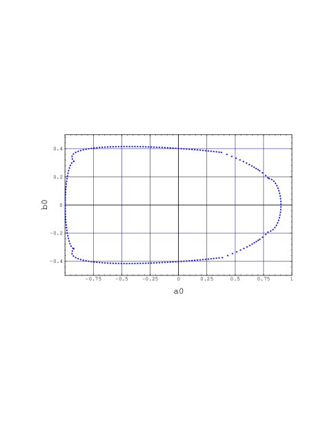
Figure 8: Combined bounds for $a_{0}\>$ and $b_{0}\>$ from the present CKM limits and with $P/T=0.055\>\>$.

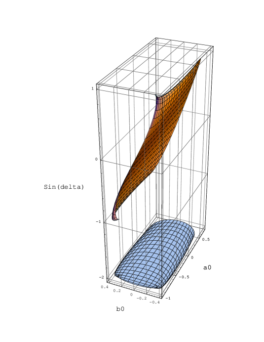
Figure 9: Expected values for $\sin\delta\>$ once  $a_{0}\>$ , $b_{0}\>$  and $\beta$ are known. The allowed domain for ( $a_{0}\>$ , $b_{0}\>$ ) from the present CKM limits and with $P/T=0.055\>\>$ is shown in the projection.

5 Conclusions

We have described a quantitative procedure to extract ( in a model-dependent way ) the value of the CKM angle $\alpha$ from a measurement of ${B^{\scriptscriptstyle 0}_{\scriptscriptstyle d}}\to{\pi^{+}}{\pi^{-}}\/$ in the presence of penguin pollution. We have shown that uncertainties of strong interaction origin can be controlled and that a model-dependent penguin correction to the measured value of $\alpha$ from ${B^{\scriptscriptstyle 0}_{\scriptscriptstyle d}}\to{\pi^{+}}{\pi^{-}}\/$ can be evaluated and parameterized in terms of the CKM angle $\beta$ and of the parameters $a_{0}\>$ and $b_{0}\>$ extracted from a time-dependent analysis. Also, the $\cos\Delta mt\>$ term in a time-dependent analysis of $\stackrel{{\scriptstyle{\scriptscriptstyle(-)}}}{{B^{\scriptscriptstyle 0}_{\scriptscriptstyle d}}}\to{\pi^{+}}{\pi^{-}}$ is found not to be sufficient to provide a direct measurement of the size of the penguin, but to provide instead useful information on the phases of strong origin.
The model-dependence of the procedure stems from the numerical dependence on the ratio of penguin-to-tree hadronic matrix elements $P/T$ (see section 2) of the penguin correction $\Delta\alpha$ (to the weak phase $\alpha$), of the corresponding correction $\Delta\mbox{$a_{0}\>$\/}$ (to the observed asymmetry $a_{0}\>$) and of the ratio $\frac{\mbox{$b_{0}\>$\/}}{\sin\delta}$.
The model-dependent procedure to extract $\alpha$ and $\delta$ proposed in this paper is applied to one final numerical example where we take the value $P/T=0.055$ from section 2 and assume for $\beta$ a measured central value of $\beta=18^{\circ}$. An observed asymmetry $\mbox{$a_{0}\>$\/}\approx-0.14$ would, in this example, require a large penguin correction $\Delta\mbox{$a_{0}\>$\/}\approx 0.32$ and the extracted “true” asymmetry value would be $\mbox{$a_{0}\>$\/}^{corrected}\approx-0.46$. In terms of $\alpha$, a correction $\Delta\alpha\approx 10^{\circ}$ should be applied to the measured central value $\mbox{${\alpha_{\scriptscriptstyle M}}$}\approx 86^{\circ}$ and would result into a “penguin corrected” value of $\alpha\approx 76^{\circ}$. An obvious comment is that a $\Delta\alpha$ correction of order $10\%$ corresponds to a significantly larger correction in terms of $\Delta\mbox{$a_{0}\>$\/}$ as a consequence of the $-\sin 2\alpha$ dependence of the asymmetry on $\alpha$. In our example, a measured central value of $\mbox{$b_{0}\>$\/}=-0.1$ would correspond to a value for the relative strong phase $\delta\approx 16^{\circ}$.
The experimental errors on the parameters $a_{0}\>$ and $b_{0}\>$ from a time-dependent analysis of ${B^{\scriptscriptstyle 0}_{\scriptscriptstyle d}}\to{\pi^{+}}{\pi^{-}}\/$, together with the expected error from an independent measurement of $\sin 2\beta$, propagate into an uncertainty on the asymmetry correction $\Delta\mbox{$a_{0}\>$\/}$ and on the extracted value of $\delta$.
The evaluation of such uncertainties as well as the assessment of the experimental sensitivities to $\alpha$ and $\delta$ is beyond the scope of the present paper.

References

- [1] For a review see, e.g., Y. Nir and H.R. Quinn, Annu. Rev. Nucl. Part. Sci. 42 (1992) 211, and references therein.
- [2] M. Gronau, Phys. Lett. B300 (1993) 163.
- [3] M. Bauer, B. Stech and M. Wirbel, Z. Phys. C 34 (1987) 103.
- [4] L. Wolfenstein, Phys. Rev. D 43 (1991) 152; and references there.
- [5] G. Kramer, W.F. Palmer and Y.L. Wu, Report DESY 95-246 (1995).
- [6] H. Simma and D. Wyler, Phys. Lett. B272 (1991) 375.
- [7] A.J. Buras and R. Fleischer, Phys. Lett. B341 (1995) 379.
- [8] M. Bander, D. Silverman and A. Soni, Phys. Rev. Lett. 43 (1979) 242.
- [9] J.F. Donoghue, E. Golowich, A. Petrov and J.M. Soares, Phys. Rev. Lett. 77 (1996) 2178.
- [10] A.N. Kamal, Int. J. Mod. Phys. A7 (1992) 3515.
- [11] B. Blok and I. Halperin, Phys. Lett. B385 (1996) 324.
- [12] M. Gronau and D. London, Phys. Rev. Lett. 65 (1990) 3381.
- [13] C. Hamzaoui and Z. Xing, Phys. Lett. B360 (1995) 131.
- [14] N.G. Deshpande and X.-G. He, Phys. Lett. B384 (1996) 283.
- [15] G. Kramer and W.F. Palmer, Phys. Rev. D 52 (1995) 6411.
- [16] A. Deandrea, N. Di Bartolomeo, R. Gatto, F. Feruglio and G. Nardulli, Phys. Lett B320 (1994) 170.
- [17] J.P. Silva and L. Wolfenstein, Phys. Rev. D 49 (1994) 1151.
- [18] Z. Xing, Nuovo Cim. A108 (1995) 1069.
- [19] N.G. Deshpande and X.-G. He, Phys. Rev. Lett. 75 (1995) 1703.
- [20] M. Gronau, O.F. Hernandéz, D. London and J.L. Rosner, Phys. Rev. D 52 (1995) 6356.
- [21] A.S. Dighe, M. Gronau and J.L. Rosner, Phys. Rev. D 54 (1996) 3309.
- [22] R. Fleischer and T. Mannel, Report TTP 96-49 (1996).
- [23] A.J. Buras and R. Fleischer, Phys. Lett. B360 (1995) 138.
- [24] F. DeJongh and P. Sphicas, Phys. Rev. D 53 (1996) 4930.
- [25] A.E. Snyder and H.R. Quinn, Phys. Rev. D 48 (1993) 2139; H.J. Lipkin, Y. Nir, H.R. Quinn and A. Snyder, Phys. Rev. D 44 (1991) 1454.
- [26] R. Aleksan, F. Buccella, A. Le Youanc, L. Oliver, O. Péne and J.-C. Raynal, Phys. Lett. B356 (1995) 95.
- [27] H. Fritzsch, D. Wu and Z. Xing, Phys. Lett. B328 (1994) 477.
- [28] D.Du and Z. Xing, Phys. Lett. B280 (1991) 292, and references therein.
- [29] A.J. Buras, M. Jamin, M.E. Lautenbacher and P.H. Weisz, Nucl. Phys. B370 (1992) 69; ibid. B400 (1993) 37; A.J. Buras, M. Jamin and M.E. Lautenbacher, Nucl. Phys. B400 (1993) 75.
- [30] M. Ciuchini, E. Franco, G. Martinelli and L. Reina, Nucl. Phys. B415 (1994) 403.
- [31] N.G. Deshpande and X.-G. He, Phys. Rev. Lett. 74 (1995) 26.
- [32] M. Gronau, O.F. Hernandéz, D. London and J.L. Rosner, Phys. Rev. D 52 (1995) 6374.
- [33] M. Bauer, B. Stech and M. Wirbel, Z. Phys. C 34 (1987) 103.
- [34] Review of Particle Properties, Phys. Rev. D 54 (1996) 1.
- [35] Y. Koide, Shizuoka report US-94-05 (1994).
- [36] A. Ali and D.London, Report DESY 96-140 (1996).
- [37] A. Ali, Report DESY 96-248 (1996).
- [38] J. Rosner, Report EFI-96-46 (1996).