Abstract

The decay $K_{L}\rightarrow\pi^{0}\gamma e^{+}e^{-}$ occurs at a higher rate than the nonradiative process $K_{L}\rightarrow\pi^{0}e^{+}e^{-}$, and hence can be a background to CP violation studies using the latter reaction. It also has an interest in its own right in the context of chiral perturbation theory, through its relation to the decay $K_{L}\rightarrow\pi^{0}\gamma\gamma$. The leading order chiral loop contribution to $K_{L}\rightarrow\pi^{0}\gamma e^{+}e^{-}$, including the $(q_{e^{+}}+q_{e^{-}})^{2}/m^{2}_{\pi}$ dependence, is completely calculable. We present this result and also include the higher order modifications which are required in the analysis of $K_{L}\rightarrow\pi^{0}\gamma\gamma$.

UMHEP-436

I. Introduction

There are three rare decay modes of the long lived kaon which have interrelated theoretical issues: $K_{L}\rightarrow\pi^{0}\gamma\gamma$, $K_{L}\rightarrow\pi^{0}e^{+}e^{-}$ and $K_{L}\rightarrow\pi^{0}\gamma e^{+}e^{-}$. The first two have been extensively studied; the latter has not been previously calculated. It is the purpose of this paper to provide a calculation of the latter process and describe how it is related to the phenomenology of the other two decays.

There is a curious and important inverted hierarchy of these decay modes. The rate for the radiative decay $K_{L}\rightarrow\pi^{0}\gamma e^{+}e^{-}$ is a power of $\alpha$ larger than the nonradiative transition $K_{L}\rightarrow\pi^{0}e^{+}e^{-}$. This is because the $K_{L}\rightarrow\pi^{0}e^{+}e^{-}$ transition occurs only through a two-photon intermediate state, or alternatively through a one-photon exchange combined with CP violation (which numerically appears to be roughly of the same size as the two-photon contribution) [1]. The $K_{L}\rightarrow\pi^{0}e^{+}e^{-}$ rate is then of order $\alpha^{4}$. However, in $K_{L}\rightarrow\pi^{0}\gamma e^{+}e^{-}$ we need only a one-photon exchange to the $e^{+}e^{-}$, leading to a rate of order $\alpha^{3}$. Our attention was first called to this inverted hierarchy by an observation that there are infrared divergences in a detailed study of the $K_{L}\rightarrow\pi^{0}e^{+}e^{-}$ two-photon effect [1] which need to be canceled by the one-loop corrections to the radiative mode $K_{L}\rightarrow\pi^{0}\gamma e^{+}e^{-}$ through the contributions of the soft radiative photons. This implies that the theoretical and experimental analyses of $K_{L}\rightarrow\pi^{0}e^{+}e^{-}$ and $K_{L}\rightarrow\gamma\pi^{0}e^{+}e^{-}$are tied together. The soft and collinear photon regions of $K_{L}\rightarrow\gamma\pi^{0}e^{+}e^{-}$ form potential backgrounds to the studies of CP violation in the $K_{L}\rightarrow\pi^{0}e^{+}e^{-}$ mode.

The $K_{L}\rightarrow\pi^{0}\gamma e^{+}e^{-}$ mode also has an interest of its own. In recent years there have been important phenomenological studies of $K_{L}\rightarrow\pi^{0}\gamma\gamma$ in connection with chiral perturbation theory (ChPTh). This decay is calculable at one-loop (i.e., order E⁴) ChPTh with no free parameters, yielding a very distinctive spectrum and a definite rate [2]. Surprisingly, when the experiment was performed the spectrum was confirmed while the measured rate was more than a factor of 2 larger than predicted. The way out of this problem appears to have been provided by Cohen, Ecker, and Pich (CEP) [3]. By adding an adjustable new effect at order E⁶, as well as including known corrections to the $K_{L}\rightarrow\pi\pi\pi$ vertex, they found that the predicted rate can be increased dramatically without modifying the shape of the spectrum much. This is also a surprising result, yet as far as we know it is the unique solution to the experimental puzzle. The ingredients of the mode studied in this paper, $K_{L}\rightarrow\pi^{0}\gamma e^{+}e^{-}$, are the same as for $K_{L}\rightarrow\pi^{0}\gamma\gamma$, except that one of the photons is off shell. Within the framework of the CEP calculation, the ingredients enter with different relative weights for off-shell photons. This will allow us to test the consistency of the theoretical resolution proposed for $K_{L}\rightarrow\pi^{0}\gamma\gamma$.

We outline the computation for the $\cal{O}$(E⁴) contribution to the process in Sec. II, and then we extend it to $\cal{O}$(E⁶) in Sec. III. Finally, we recapitulate our conclusions in Sec. IV.

II. The $\cal{O}$(E⁴) calculation

First let us provide the straightforward $\cal{O}$(E⁴) calculation within ChPTh. This is the generalization to $k^{2}_{1}\neq 0$ of the original chiral calculation of EPR [2]. Here $k_{1}$ is the momentum of the off-shell photon. This captures all the $k^{2}_{1}/m^{2}_{\pi}$ and $k^{2}_{1}/m^{2}_{K}$ variations of the amplitudes at this order in the energy expansion. There can be further $k^{2}_{1}$/(1 GeV)² corrections which correspond to $\cal{O}$(E⁶) and higher. The easiest technique for this calculation uses the basis where the kaon and pion fields are transformed so that the propagators have no off-diagonal terms, as described in ref. [2]. The relevant diagrams are then shown in Fig. 1. Defining $\overline{g}$ as

$${\overline{g}}=G^{\phantom{l}}_{8}/3,\qquad\qquad G^{\phantom{l}}_{8}=G^{\phantom{l}}_{F}|V_{ud}^{\phantom{*}}V_{us}^{*}|g^{\phantom{l}}_{8},\qquad\qquad|g^{\phantom{l}}_{8}|\approx 5.1,$$ (1)

the diagrams give the following integrals, respectively:

$${\cal M}^{a}_{\mu\nu}=2e^{2}{\overline{g}}g_{\mu\nu}\int{{d^{4}l}\over{(2\pi)^{4}}}{{3[(p^{\phantom{l}}_{K}-p^{\phantom{l}}_{0})^{2}-m^{2}_{\pi}]-2[(l^{2}-m^{2}_{\pi})+(l-k_{1}-k_{2})^{2}-m^{2}_{\pi}]}\over{(l^{2}-m^{2}_{\pi})[(l-k_{1}-k_{2})^{2}-m^{2}_{\pi}]}},$$ (2)

$${\cal M}^{b}_{\mu\nu} = -e^{2}{\overline{g}}\int{{d^{4}l}\over{(2\pi)^{4}}}{{3[(p^{\phantom{l}}_{K}-p^{\phantom{l}}_{0})^{2}-m^{2}_{\pi}]-2[(l+k_{1})^{2}-m^{2}_{\pi}+(l-k_{2})^{2}-m^{2}_{\pi}]}\over{(l^{2}-m^{2}_{\pi})[(l+k_{1})^{2}-m^{2}_{\pi}][(l-k_{2})^{2}-m^{2}_{\pi}]}}$$ (3)

$$\times (2l+k_{1})_{\mu}(2l-k_{2})_{\nu}+(k_{1},\mu)\leftrightarrow(k_{2},\nu),$$

$${\cal M}^{c}_{\mu\nu}=8e^{2}{\overline{g}}g_{\mu\nu}\int{{d^{4}l}\over{(2\pi)^{4}}}{1\over{l^{2}-m^{2}_{\pi}}},$$ (4)

$${\cal M}^{d}_{\mu\nu}=-4e^{2}{\overline{g}}\int{{d^{4}l}\over{(2\pi)^{4}}}\left\{{{(2l-k_{1})_{\mu}(2l-k_{1})_{\nu}}\over{(l^{2}-m^{2}_{\pi})[(l-k_{1})^{2}-m^{2}_{\pi}]}}+{{(2l-k_{2})_{\mu}(2l-k_{2})_{\nu}}\over{(l^{2}-m^{2}_{\pi})[(l-k_{2})^{2}-m^{2}_{\pi}]}}\right\}.$$ (5)

Figure 1: Diagrams relevant to the process $K_{L}\rightarrow\pi^{0}\gamma e^{+}e^{-}$ at ${\cal O}(E^{4})$ and ${\cal O}(E^{6})$.

Interestingly when we add these together the $K\rightarrow 3\pi$ amplitude factors out from the remaining loop integral resulting in

$${\cal M}^{\pi}_{\mu\nu}=6e^{2}{\overline{g}}[(p^{\phantom{l}}_{K}-p^{\phantom{l}}_{0})^{2}-m^{2}_{\pi}]\int{{d^{4}l}\over{(2\pi^{4})}}{{[g_{\mu\nu}(l^{2}-m^{2}_{\pi})-(2l+k_{1})_{\mu}(2l-k_{2})_{\nu}]}\over{{(l^{2}-m^{2}_{\pi})[(l+k_{1})^{2}-m^{2}_{\pi}][(l-k_{2})^{2}-m^{2}_{\pi}]}}}.$$ (6)

It is not hard to verify that this result satisfies the constraints of gauge invariance $k^{\mu}_{1}\cal{M}_{\mu\nu}$ = $k^{\nu}_{2}\cal{M}_{\mu\nu}$ = 0. At this stage, the integral may be parametrized and integrated using standard Feynman-diagram techniques. Let us keep photon number one as the off-shell photon and set $k^{2}_{2}=0$. In this case the amplitude with one photon off-shell is described by

$${\cal M}^{\pi}_{\mu\nu}=6e^{2}{\overline{g}}[(p^{\phantom{l}}_{K}-p^{\phantom{l}}_{0})^{2}-m^{2}_{\pi}]\left({-i}\over{16\pi^{2}}\right){{(g_{\mu\nu}k_{1}\cdot k_{2}-k_{2\mu}k_{1\nu})}\over{k_{1}\cdot k_{2}}}[1+2I(m^{2}_{\pi})],$$ (7)

with

$$I(m^{2}_{\pi}) = \int^{1}_{0}dz_{1}\int_{0}^{1-z_{1}}dz_{2}{{m^{2}_{\pi}-z_{1}(1-z_{1})k^{2}_{1}}\over{2z_{1}z_{2}k_{1}\cdot k_{2}+z_{1}(1-z_{1})k^{2}_{1}-m^{2}_{\pi}+i\epsilon}}$$ (8)

$$= {m^{2}_{\pi}\over{s-k^{2}_{1}}}[F(s)-F(k^{2}_{1})]-{k^{2}_{1}\over{s-k^{2}_{1}}}[G(s)-G(k^{2}_{1})].$$

The notation is defined by

$$s=(p^{\phantom{l}}_{K}-p^{\phantom{l}}_{0})^{2}=(k_{1}+k_{2})^{2}$$ (9)

and

$$F(a)=\int^{1}_{0}{dz_{1}\over z_{1}}\log\left[{{m^{2}_{\pi}-a(1-z_{1})z_{1}-i\epsilon}\over{m^{2}_{\pi}}}\right],$$ (10)

$$G(a)=\int^{1}_{0}dz_{1}\log\left[{{m^{2}_{\pi}-a(1-z_{1})z_{1}-i\epsilon}\over{m^{2}_{\pi}}}\right].$$ (11)

The above functions are related to those presented by CEP [3]:

$$F(a)={a\over{2m^{2}_{\pi}}}\left[F_{\rm CEP}\left({a\over 4m^{2}_{\pi}}\right)-1\right],$$ (12)

$$G(a)=-{a\over{2m^{2}_{\pi}}}\left[R_{\rm CEP}\left({a\over 4m^{2}_{\pi}}\right)+{1\over 6}\right],$$ (13)

remembering that

$$F_{\rm CEP}(x) = 1-{1\over x}\left[\sin^{-1}\left(\sqrt{x}\right)\right]^{2},\,\qquad x\leq 1,$$

$$= 1+{1\over 4x}\left[\log{1-\sqrt{1-1/x}\over 1+\sqrt{1-1/x}}+i\pi\right]^{2},\,\qquad x\geq 1,$$

$$R_{\rm CEP}(x) = -{1\over 6}+{1\over 2x}\left[1-\sqrt{1/x-1}\sin^{-1}\left(\sqrt{x}\right)\right],\,\qquad x\leq 1,$$ (14)

$$-{1\over 6}+{1\over 2x}\left[1+\sqrt{1-1/x}\left(\log{1-\sqrt{1-1/x}\over 1+\sqrt{1-1/x}}+i\pi\right)\right],\,\qquad x\geq 1.$$

This agrees with the EPR result in the $k^{2}_{1}\rightarrow 0$ limit.

At this order we have also calculated the additional contribution resulting from the kaons circulating in the loops of Fig. 1. They give rise to

$${\cal M}^{K}_{\mu\nu}=6e^{2}{\overline{g}}(m^{2}_{K}+m^{2}_{\pi}-s)\int{{d^{4}l}\over{(2\pi^{4})}}{{[g_{\mu\nu}(l^{2}-m^{2}_{K})-(2l+k_{1})_{\mu}(2l-k_{2})_{\nu}]}\over{{(l^{2}-m^{2}_{K})[(l+k_{1})^{2}-m^{2}_{K}][(l-k_{2})^{2}-m^{2}_{K}]}}}.$$ (15)

The resulting integral is similar to that of Eq. (8), substituting the mass of the pion with that of the kaon. Attaching an $e^{+}e^{-}$ couple to either photon and adding all the above contributions together, the result we obtain for the branching ratio is

$${\rm BR}(K_{L}\rightarrow\pi^{0}\gamma e^{+}e^{-})=1.0\times 10^{-8}.$$ (16)

With the definitions

$$z={s\over{m^{2}_{K}}},\qquad y={{p^{\phantom{l}}_{K}\cdot(k_{1}-k_{2})}\over{m^{2}_{K}}},$$ (17)

the decay distributions in $z$ and $y$ provide more detailed information. We present them in Figs. 2 and 3.

Figure 2: Differential branching ratio $d\Gamma(K_{L}\rightarrow\pi^{0}\gamma e^{+}e^{-})/dz$ to order ${\cal O}$(E⁴).

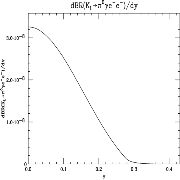
Figure 3: Differential branching ratio $d\Gamma(K_{L}\rightarrow\pi^{0}\gamma e^{+}e^{-})/dy$ to order ${\cal O}$(E⁴).

III. The $\cal{O}$(E⁶) calculation

We also wish to extend this calculation along the lines proposed by CEP [3], who provide a plausible solution to the problem raised by the experimental rate not agreeing with the $\cal{O}$(E⁴) calculation when both photons are on-shell. The two primary new ingredients involve known physics which surfaces at the next order in the energy expansion. The first involves the known quadratic energy variation of the $K\rightarrow 3\pi$ amplitude, which occurs from higher order terms in the weak nonleptonic Lagrangian [4, 5]. While the full one-loop structure of this is known [6], it involves complicated nonanalytic functions and we approximate the result at $\cal{O}$(E⁴) by an analytic polynomial which provides a good description of the data throughout the physical region:

$${\cal M}(K\rightarrow\pi^{+}\pi^{-}\pi^{0})=4a_{1}p^{\phantom{l}}_{K}\cdot p^{\phantom{l}}_{0}p^{\phantom{l}}_{+}\cdot p^{\phantom{l}}_{-}+4a_{2}(p^{\phantom{l}}_{K}\cdot p^{\phantom{l}}_{+}p^{\phantom{l}}_{0}\cdot p^{\phantom{l}}_{-}+p^{\phantom{l}}_{K}\cdot p^{\phantom{l}}_{-}p^{\phantom{l}}_{0}\cdot p^{\phantom{l}}_{+}),$$ (18)

using

$$a_{1}=3.1\times 10^{-6}m^{-4}_{K}\qquad{\rm and}\qquad a_{2}=-1.26\times 10^{-6}m^{-4}_{K}.$$ (19)

$a_{1}$ and $a_{2}$ are obtained from a fit to the amplitude for $K_{L}\rightarrow\pi^{0}\pi^{+}\pi^{-}$ [4] and to the amplitude and spectrum for $K_{L}\rightarrow\pi^{0}e^{+}e^{-}$ [3], so that their values are constrained within their theoretical uncertainty of 10 – 20%. We have numerically verified that such a variation of said parameters involves a very modest change in the shape of the spectrum for $K_{L}\rightarrow\gamma\pi^{0}e^{+}e^{-}$ and a change in its final branching ratio somewhat smaller than the uncertainty on the parameters.

The other ingredient involves vector meson exchange such as in Fig. 4. Some of such contributions are known, but there are others such as those depicted in Fig. 5 which have the same structure but an unknown strength, leaving the total result unknown. In Ref. [3] the result is parametrized by a “subtraction constant” which must be fit to the data.

Figure 4: Vector meson exchange diagrams contributing to $K_{L}\rightarrow\pi^{0}\gamma e^{+}e^{-}$.

Figure 5: Vector meson exchange diagrams contributing to $K_{L}\rightarrow\pi^{0}\gamma e^{+}e^{-}$ with unknown strength.

In principle one can add the ingredients to the amplitudes and perform a dispersive calculation of the total transition matrix element. In practice it is simple to convert the problem to an effective field theory and and do a Feynman diagram calculation which will yield the same result. We follow this latter course.

The Feynman diagrams are the same as shown in Fig. 1, although the vertices are modified by the presence of $\cal{O}$(E⁴) terms in the energy expansion. Not only does the direct $K\rightarrow 3\pi$ vertex change to the form given in Eq. (18), but also the weak vertices with one and two photons have a related change. The easiest way to determine these is to write a gauge invariant effective Lagrangian with coefficients adjusted to reproduce Eq. (18). We find

$${\cal M_{\mu}}(K\rightarrow\pi^{+}\pi^{-}\pi^{0}\gamma)=4a_{1}e(p^{\phantom{l}}_{+}-p^{\phantom{l}}_{-})_{\mu}+4a_{2}e(p^{\phantom{l}}_{+}-p^{\phantom{l}}_{-})_{\sigma}(p^{\sigma}_{0}p^{\phantom{l}}_{K\mu}+p^{\sigma}_{K}p^{\phantom{l}}_{0\mu}),$$ (20)

$${\cal M}_{\mu\nu}(K\rightarrow\pi^{+}\pi^{-}\pi^{0}\gamma\gamma)=-8a_{1}e^{2}g_{\mu\nu}p^{\phantom{l}}_{K}\cdot p^{\phantom{l}}_{0}+8a_{2}e^{2}(p^{\phantom{l}}_{K\mu}p^{\phantom{l}}_{0\nu}+p^{\phantom{l}}_{K\nu}p^{\phantom{l}}_{0\mu}).$$ (21)

The resulting calculation follows the same steps as described above, but is more involved and is not easy to present in a simple form. We have checked that our result is gauge invariant and reduces to that of CEP in the limit of on-shell photons.

The contribution proportional to $a_{1}$ can be computed analogously to those already calculated for the $\cal{O}$(E⁴) case:

$${\cal M}_{\mu\nu}=4a_{1}e^{2}(z-2r^{2}_{\pi})(1+r^{2}_{\pi}-z){1\over{(z-q)}}(g_{\mu\nu}k_{1}\cdot k_{2}-k_{2\mu}k_{1\nu})[1+2I(m^{2}_{\pi})],$$ (22)

where

$$r_{\pi}={m_{\pi}\over m_{K}},\qquad z={s\over{m^{2}_{K}}},\qquad q={{k^{2}_{1}}\over{m^{2}_{K}}}.$$ (23)

The $a_{2}$ part originates another set of integrals which can be written as

$${\cal M}^{a}_{\mu\nu}=-8a_{2}(p^{\rho}_{K}p^{\sigma}_{0}+p^{\sigma}_{K}p^{\rho}_{0})e^{2}g_{\mu\nu}\int{{d^{d}l}\over{(2\pi)^{d}}}{{l_{\rho}(l-k_{1}-k_{2})_{\sigma}}\over{(l^{2}-m^{2}_{\pi})[(l-k_{1}-k_{2})^{2}-m^{2}_{\pi}]}},$$ (24)

$${\cal M}^{b}_{\mu\nu} = 4a_{2}(p^{\rho}_{K}p^{\sigma}_{0}+p^{\sigma}_{K}p^{\rho}_{0})e^{2}\int{{d^{d}l}\over{(2\pi)^{d}}}\left\{{{(2l+k_{1})_{\mu}(2l-k_{2})_{\nu}(l+k_{1})_{\rho}(l-k_{2})_{\sigma}}\over{(l^{2}-m^{2}_{\pi})[(l+k_{1})^{2}-m^{2}_{\pi}][(l-k_{2})^{2}-m^{2}_{\pi}]}}\right.$$ (25)

$$+ \left.{{(2l+k_{2})_{\nu}(2l-k_{1})_{\mu}(l+k_{2})_{\rho}(l-k_{1})_{\sigma}}\over{(l^{2}-m^{2}_{\pi})[(l-k_{1})^{2}-m^{2}_{\pi}][(l+k_{2})^{2}-m^{2}_{\pi}]}}\right\}$$

$$= 8a_{2}(p^{\rho}_{K}p^{\sigma}_{0}+p^{\sigma}_{K}p^{\rho}_{0})e^{2}\int{{d^{d}l}\over{(2\pi)^{d}}}{{(2l+k_{1})_{\mu}(2l-k_{2})_{\nu}(l+k_{1})_{\rho}(l-k_{2})_{\sigma}}\over{(l^{2}-m^{2}_{\pi})[(l+k_{1})^{2}-m^{2}_{\pi}][(l-k_{2})^{2}-m^{2}_{\pi}]}},$$

$${\cal M}^{c}_{\mu\nu}=8a_{2}(p^{\phantom{l}}_{K\mu}p^{\phantom{l}}_{0\nu}+p^{\phantom{l}}_{K\nu}p^{\phantom{l}}_{0\mu})e^{2}\int{{d^{d}l}\over{(2\pi)^{d}}}{1\over{l^{2}-m^{2}_{\pi}}},$$ (26)

$${\cal M}^{d}_{\mu\nu} = -4a_{2}(p^{\sigma}_{0}p^{\phantom{l}}_{K\nu}+p^{\sigma}_{K}p^{\phantom{l}}_{0\nu})e^{2}\int{{d^{d}l}\over{(2\pi)^{d}}}{{(2l-k_{1})_{\mu}(2l-k_{1})_{\sigma}}\over{(l^{2}-m^{2}_{\pi})[(l-k_{1})^{2}-m^{2}_{\pi}]}}$$ (27)

$$- 4a_{2}(p^{\sigma}_{0}p^{\phantom{l}}_{K\mu}+p^{\sigma}_{K}p^{\phantom{l}}_{0\mu})e^{2}\int{{d^{d}l}\over{(2\pi)^{d}}}{{(2l-k_{2})_{\nu}(2l-k_{2})_{\sigma}}\over{(l^{2}-m^{2}_{\pi})[(l-k_{2})^{2}-m^{2}_{\pi}]}}.$$

From the above formulas we obtain

$${\cal M}_{\mu\nu} = {1\over{(4\pi)^{2}}}\left[A(x_{1},x_{2})(k_{2\mu}k_{1\nu}-k_{1}\cdot k_{2}g_{\mu\nu})\phantom{{k^{2}_{1}}\over{k_{1}}}\right.$$ (28)

$$+ B(x_{1},x_{2})\left({p^{\phantom{l}}_{K}\cdot k_{1}p^{\phantom{l}}_{K}\cdot k_{2}\over{k_{1}\cdot k_{2}}}g_{\mu\nu}+p^{\phantom{l}}_{K\mu}p_{K\nu}-{{p^{\phantom{l}}_{K}\cdot k_{1}}\over{k_{1}\cdot k_{2}}}k_{2\mu}p^{\phantom{l}}_{K\nu}-{{p^{\phantom{l}}_{K}\cdot k_{2}}\over{k_{1}\cdot k_{2}}}k_{1\nu}p^{\phantom{l}}_{K\mu}\right)$$

$$+ \left.D(x_{1},x_{2})\left(k^{2}_{1}{p^{\phantom{l}}_{K}\cdot k_{2}\over{k_{1}\cdot k_{2}}}g_{\mu\nu}-{{p^{\phantom{l}}_{K}\cdot k_{2}}\over{k_{1}\cdot k_{2}}}k_{1\mu}k_{1\nu}+k_{1\mu}p^{\phantom{l}}_{K\nu}-{{k^{2}_{1}}\over{k_{1}\cdot k_{2}}}k_{2\mu}p^{\phantom{l}}_{K\nu}\right)\right],$$

where

$$A = 16a_{2}e^{2}\{2[1-2(x_{1}+x_{2})]I_{1}(z_{1}z_{2})+x_{1}I_{1}(z_{2})+x_{2}[2I_{1}(z^{2}_{2})-I_{1}(z_{2})+I_{1}(z_{1})]\}$$

$$- 32a_{2}e^{2}\{[2x^{2}_{1}-x_{1}(z+q)][-I_{2}(z^{3}_{1}z_{2})+I_{2}(z^{2}_{1}z_{2})]$$

$$+ [2x_{1}x_{2}-x_{1}(z-q)/2-x_{2}(z+q)/2][2I_{2}(z^{2}_{1}z^{2}_{2})+I_{2}(z_{1}z_{2})-I_{2}(z^{2}_{1}z_{2})$$

$$- I_{2}(z_{1}z^{2}_{2})]+[2x^{2}_{2}-x_{2}(z-q)][I_{2}(z_{1}z^{2}_{2})-I_{2}(z_{1}z^{3}_{2})]\}$$

$$+ {4\over 3}a_{2}e^{2}\log{m^{2}_{\pi}\over{m^{2}_{\rho}}}+(4\pi)^{2}{\rm VMD}_{A},$$

$$B=-32a_{2}e^{2}I_{3}+16a_{2}I_{4}+{4\over 3}a_{2}e^{2}(z-q)\left(-1+\log{m^{2}_{\pi}\over{m^{2}_{\rho}}}\right)+(4\pi)^{2}{\rm VMD}_{B},$$ (30)

$$D= - {B\over 2}+16a_{2}e^{2}[2x_{2}-(z-q)/2][2I_{1}(z_{1}z_{2})-I_{1}(z_{2})]$$ (31)

$$+ 16a_{2}e^{2}(2y-q)[I_{1}(z_{1})-I_{1}(1)/2]+4a_{2}e^{2}[2x_{1}-(z+q)/2]I_{5}$$

$$+ (4\pi)^{2}{\rm VMD}_{D},$$

with

$$I_{1}(z^{n}_{1}z^{m}_{2})=\int^{1}_{0}dz_{1}\int^{1-z_{1}}_{0}dz_{2}z^{n}_{1}z^{m}_{2}\log{D_{1}\over{m^{2}_{\pi}}},$$ (32)

$$I_{2}(z^{n}_{1}z^{m}_{2})=\int^{1}_{0}dz_{1}\int^{1-z_{1}}_{0}dz_{2}{{z^{n}_{1}z^{m}_{2}}\over D_{1}},$$ (33)

$$I_{3}=\int^{1}_{0}dz_{1}\int^{1-z_{1}}_{0}dz_{2}D_{1}\log{D_{1}\over{m^{2}_{\pi}}},$$ (34)

$$I_{4}=\int^{1}_{0}dz_{1}D_{2}\log{D_{2}\over{m^{2}_{\pi}}},$$ (35)

$$I_{5}=\int^{1}_{0}dz_{1}(4z^{2}_{1}-4z_{1}+1)\log{D_{2}\over{m^{2}_{\pi}}},$$ (36)

and

$$D_{1} = m^{2}_{\pi}-2k_{1}\cdot k_{2}z_{1}z_{2}-k^{2}_{1}z_{1}(1-z_{1}),$$

$$D_{2} = m^{2}_{\pi}-k^{2}_{1}z_{1}(1-z_{1}),$$

$$x_{1} = {{p^{\phantom{l}}_{K}\cdot k_{1}}\over{m^{2}_{K}}},\qquad x_{2}={{p^{\phantom{l}}_{K}\cdot k_{2}}\over{m^{2}_{K}}},$$ (37)

$${\rm VMD}_{A}(x_{1},x_{2})=-\sum_{V=\omega,\rho}G_{V}\left[{{p^{\phantom{l}}_{K}\cdot(p^{\phantom{l}}_{K}-k_{2})}\over{(p^{\phantom{l}}_{K}-k_{2})^{2}-m^{2}_{V}}}+{{p^{\phantom{l}}_{K}\cdot(p^{\phantom{l}}_{K}-k_{1})}\over{(p^{\phantom{l}}_{K}-k_{1})^{2}-m^{2}_{V}}}\right],$$ (38)

$${\rm VMD}_{B}(x_{1},x_{2})=-\sum_{V=\omega,\rho}G_{V}k_{1}\cdot k_{2}\left[{1\over{(p^{\phantom{l}}_{K}-k_{2})^{2}-m^{2}_{V}}}+{1\over{(p^{\phantom{l}}_{K}-k_{1})^{2}-m^{2}_{V}}}\right],$$ (39)

$${\rm VMD}_{D}(x_{1},x_{2})=\sum_{V=\omega,\rho}G_{V}{{k_{1}\cdot k_{2}}\over{(p^{\phantom{l}}_{K}-k_{1})^{2}-m^{2}_{V}}},$$ (40)

assuming the numerical values [7]

$$G_{\rho}m^{2}_{K}=0.68\times 10^{-8},\qquad G_{\omega}m^{2}_{K}=-0.28\times 10^{-7}.$$ (41)

The loop calculation that we have just described provides all of the off-shell dependence scaled by the pion mass, and is of the form $k^{2}_{1}/m^{2}_{\pi}$. There can be an additional dependence of the form $k^{2}_{1}/\Lambda^{2}$, where $\Lambda$ $\approx$ 1 GeV. We cannot provide a model independent analysis of the latter. However, experience has shown that most of the higher order momentum dependence is well accounted for by vector meson exchange. Therefore we include the $k^{2}_{1}/\Lambda^{2}$ dependence which is predicted by the diagrams of Fig. 4. One can recover the parametrization in $a_{V}$ neglecting the dependence on $(p^{\phantom{l}}_{K}-k_{1})^{2}$ and $(p^{\phantom{l}}_{K}-k_{2})^{2}$ in formulas (38) – (40), and performing the replacement [7]

$${{\pi G_{\rm eff}m^{2}_{K}}\over{2G_{8}\alpha m^{2}_{V}}}\rightarrow a_{V},$$ (42)

where $G_{\rm eff}$ $\approx$ $G_{\rho}$+$G_{\omega}$. This completes our treatment of the $K_{L}\rightarrow\pi^{0}\gamma e^{+}e^{-}$ amplitude.

The calculation we have presented in this section leads to the total branching ratio of

$${\rm BR}(K_{L}\rightarrow\pi^{0}\gamma e^{+}e^{-})=2.3\times 10^{-8}.$$ (43)

The decay distributions are presented in Figs. 6 and 7.

Figure 6: Differential branching ratio $d\Gamma(K_{L}\rightarrow\pi^{0}\gamma e^{+}e^{-})/dz$ to order ${\cal O}$(E⁶).

Figure 7: Differential branching ratio $d\Gamma(K_{L}\rightarrow\pi^{0}\gamma e^{+}e^{-})/dy$ to order ${\cal O}$(E⁶).

IV. Conclusions

The behavior of the $K_{L}\rightarrow\pi^{0}\gamma e^{+}e^{-}$ amplitude mirrors closely that of the process $K_{L}\rightarrow\pi^{0}\gamma\gamma$. The more complete calculation at order E⁶ gives a rate which is more than twice as large as the one obtained at order E⁴, despite the fact that the new parameter introduced at order E⁶ is quite reasonable in magnitude. This large change occurs partially because the order E⁴ calculation is purely a loop effect, while at order E⁶ we have tree level contributions, and loop contributions are generally smaller than tree effects at a given order. It was more surprising that the spectrum in $K_{L}\rightarrow\pi^{0}\gamma\gamma$ was not significantly modified by the order E⁶ contributions. These new effects are more visible in the low $z$ region of the process we have calculated, $K_{L}\rightarrow\pi^{0}\gamma e^{+}e^{-}$.

This reaction should be reasonably amenable to experimental investigation in the future. It is 3–4 orders of magnitude larger than the reaction $K_{L}\rightarrow\pi^{0}e^{+}e^{-}$ which is one of the targets of experimental kaon decay programs, due to the connections of the latter reaction to CP studies. In fact, the radiative process of this paper will need to be studied carefully before the nonradiative reaction can be isolated. The regions of the distributions where the experiment misses the photon of the radiative process can potentially be confused with $K_{L}\rightarrow\pi^{0}e^{+}e^{-}$ if the resolution is not sufficiently precise. In addition, since the $\pi^{0}$ is detected through its decay to two photons, there is potential confusion related to misidentifying photons. The study of the reaction $K_{L}\rightarrow\pi^{0}\gamma e^{+}e^{-}$ will be a valuable preliminary to the ultimate CP tests.

References

[1]
J. F. Donoghue and F. Gabbiani, Phys. Rev. D 51 2187 (1995).
[2]
G. Ecker, A. Pich and E. de Rafael, Nucl. Phys. B 291 692 (1987);
Nucl. Phys. B 303 665 (1988).
[3]
A. G. Cohen, G. Ecker and A. Pich, Phys. Lett. B 304 347 (1993).
[4] J. F. Donoghue, E. Golowich and B. R. Holstein, Phys. Rev. D 30 587 (1984).
[5] L. Cappiello, G. D’Ambrosio and M. Miragliuolo, Phys. Lett. B 298 423 (1993); G. D’Ambrosio, G. Ecker, G. Isidori and
H. Neufeld, hep-ph/9411439, published in The Second DANE
Physics Handbook, ed. L. Maiani, G. Pancheri and N. Paver, INFN,
Frascati, Italy, 265 (1995); G. D’Ambrosio and G. Isidori,
hep-ph/9611284 (unpublished).
[6] J. Kambor, J. Missimer and D. Wyler, Nucl. Phys. B 346 17 (1990); J. Kambor, J. Missimer and D. Wyler, Phys. Lett. B 261 496 (1991);
J. F. Donoghue and B. R. Holstein, Phys. Rev. Lett. 68 1818 (1992).
[7] P. Heiliger and L. M. Sehgal, Phys. Rev. D 47 4920 (1993).