HOW MUCH OF THE NUCLEON SPIN
IS CARRIED BY GLUE?

Abstract

We estimate in the QCD sum rule approach the amount of the nucleon spin carried by the gluon angluar momentum: the sum of the gluon spin and orbital angular momenta. The result indicates that gluons contribute at least one half of the nucleon spin at scale of 1 GeV².

Ever since the publication of the EMC measurement on the fraction of the nucleon spin carried by the quark spin[1], there has been a tremendous activity in the field of the spin structure of the nucleon[2]. One of the central questions is how the spin of the nucleon is distributed among its constituents[3]. After much debate, many agree now that a substential fraction of the nucleon spin comes from sources other than the quark spin, i.e., quark orbital and gluon angular momenta. Recently, several proposals have been made in the literature to measure the amount of the spin carried by the gluon helicity $\Delta G$[4].

In this Letter, we present a QCD sum rule calculation [5] of the amount of the nucleon spin carried by gluons, or equivalently by quarks because, by definition, their sum is 1/2. Our calculation is motivated by the possibility of measuring these quantities through deeply-virtual Compton scattering proposed by one of us [6]. The method we use has been applied successfully to calculate a similar quantity—fractions of the nucleon momentum carried by quarks and gluons [7, 8]. Our result shows that the gluon angular momentum, the sum of gluon helicity and orbitial angular momentum, contributes at least 50% of the nucleon spin, suggesting that the nucleon contains nontrivial gluon configurations carrying nonzero angular momentum.

The angular momentum operator in QCD can be written in an explicitly gauge invariant form [6],

$$\vec{J}_{\rm QCD} = \int d^{3}x~{}\Big{[}~{}{1\over 2}\bar{\psi}\vec{\gamma}\gamma_{5}\psi+\psi^{\dagger}(\vec{x}\times(-i\vec{D}))\psi$$ (1)

$$+ \vec{x}\times(\vec{E}\times\vec{B})\Big{]}\ .$$ (2)

where flavor and color indices are implicit. The first term can be interpreted as the quark spin contribution, although its matrix element is actually the singlet axial charge. The second term, where the covariant derivative is ${\vec{D}}=\vec{\partial}+ig\vec{A}$, is the canonical orbital angular momentum of quarks. The word “canonical” stems from the canonical momentum for quarks in a background gauge field. The last term is the total angular momentum of gluons, as is clear from the appearance of the Poynting vector. [In pure gauge theory without quarks, this term generates the spin quantum numbers for glueballs]. According to the above expression, we can write down a gauge-invariant spin sum rule for the nucleon,

$${1\over 2}={1\over 2}\Delta\Sigma(\mu^{2})+L_{q}(\mu^{2})+J_{g}(\mu^{2})\ ,$$ (3)

where $\mu^{2}$ is a scale at which the operators are renormalized, or more physically the nucleon wave function is probed. The first term is what has been measured in polarized deep-inelastic scattering [1, 9]. The second and third terms represent quark orbital and gluon contributions, respectively. We also introduce the notion of the total quark contribution, $J_{q}=\Delta\Sigma/2+L_{q}$, the sum of spin and orbital. By definition, both $J_{q}(\mu^{2})$ and $J_{g}(\mu^{2})$ are gauge-invariant if gauge-invariant regularization and renormalization schemes are used. In the light-like gauge $A^{+}=0$, $J_{g}(\mu^{2})$ can be written as a sum of the gluon helicity $\Delta G(\mu^{2})$, measurable in polarized high-energy scattering[4], the gluon orbital angular momentum, as well as a term from quark-gluon interactions [6].

Before formulating the sum rule calculation, it is instructive to review a derivation of Eq. (1). The angular momentum operators of QCD are identified with the generators of the Lorentz group: $J^{\mu\nu}$, which in turn are defined from the angular momentum density $M^{\mu\nu\alpha}$ through,

$$J^{\mu\nu}=\int d^{3}\vec{x}~{}M^{0\mu\nu}(\vec{x})\ .$$ (4)

The angular momentum density can be expressed in terms of the symmetric, conserved energy-momentum tensor $T^{\alpha\beta}$,

$$M^{\mu\nu\alpha}=T^{\mu\alpha}x^{\nu}-T^{\mu\nu}x^{\alpha}\ .$$ (5)

The energy-momentum tensor of QCD can be written as a sum of the quark and gluon parts,

$$T^{\alpha\beta}=T_{q}^{\alpha\beta}+T_{g}^{\alpha\beta}={1\over 4}\bar{\psi}\gamma^{(\alpha}i\stackrel{{\scriptstyle\leftrightarrow}}{{D^{\beta)}}}\psi+\left({1\over 4}g^{\alpha\beta}F^{2}-F^{\alpha\mu}F^{\beta}_{~{}\mu}\right)\ ,$$ (6)

where $(\alpha\beta)$ means symmetrization of the indices. It is then simple to see that the quark and gluon parts of the angular momentum operators in Eq. (1) are derived from Eqs. (4) and (5) by substituting in the quark and gluon parts of the energy-momentum tensor, respectively.

According to the above, we can formulate the sum rule calculation of $J_{g}(\mu^{2})$, or equivalently $J_{q}(\mu^{2})$, in terms of the energy-momentum tensor $T^{\alpha\beta}_{q,g}$. Consider the following three-point correlation function in the QCD vacuum,

$$W^{\mu\nu\alpha}_{g}(p)=\int d^{4}xd^{4}z~{}\langle 0|T[\eta(x)\bar{\eta}(0)M^{\mu\nu\alpha}_{g}(z)]|0\rangle~{}e^{ip\cdot x}\ ,$$ (7)

where $M_{g}^{\mu\nu\alpha}$ is defined as in Eq. (5) with $T^{\alpha\beta}$ replaced by its gluonic part, and $\eta(x)$ is the interpolating field for the nucleon, which we choose to be [11],

$$\eta(x)=\epsilon^{ijk}\left(u^{iT}C\gamma^{\alpha}u^{j}\right)\gamma_{5}\gamma_{\alpha}d^{k}\ .$$ (8)

$W^{\mu\nu\alpha}$ contains a nucleon double-pole contribution, with its residue proportional to $J_{g}(\mu^{2})$,

$$W^{\mu\nu\alpha}_{g}={J_{g}(\mu^{2})\lambda_{N}^{2}\over(p^{2}-m_{N}^{2})^{2}}(2ip^{\mu}\gamma^{\nu}\mathrel{\mathop{p\!\!\!/}}\gamma^{\alpha})+...\ ,$$ (9)

where ellipses include nucleon double poles of different Dirac structures, nucleon single poles, and other dispersive contributions. $\lambda_{N}$ is the nucleon decay constant corresponding to the interpolating current,

$$\langle 0|\eta(0)|N(p)\rangle=\lambda_{N}U(p)\ .$$ (10)

In the following, we first calculate $W^{\mu\nu\alpha}$ in the deep-Euclidean region $-p^{2}>\!>\Lambda_{\rm QCD}^{2}$ using operator product expansion (OPE), from which we attempt to extract the double-pole residue $J_{g}(\mu^{2})$.

To ensure $J_{q}(\mu^{2})+J_{g}(\mu^{2})=1/2$ in the sum rule calculation, we use an implicit form of Ward identity,

$$T^{\alpha\beta}=\partial_{\rho}(T^{\rho\beta}x^{\alpha})-x^{\alpha}\partial_{\rho}T^{\rho\beta}\ ,$$ (11)

to we rewrite the three-point correlation function as,

$$W^{\mu\nu\alpha}_{g}=\int d^{4}xd^{4}z~{}\langle 0|T\eta(x)\bar{\eta}(0)z^{\mu}\left(z^{\alpha}\partial_{\rho}T^{\rho\nu}_{g}-z^{\nu}\partial_{\rho}T^{\rho\alpha}_{g}\right)|0\rangle e^{ip\cdot x}\ .$$ (12)

From Eq. (6), we find,

$$\partial_{\rho}T^{\rho\nu}_{g}=-\bar{\psi}gF^{\nu\alpha}\gamma_{\alpha}\psi+...\ ,$$ (13)

where ellipses denote terms vanishing after using gluon’s equations of motion. Thus, we arrive at a new form of the Green’s function

$$W^{\mu\nu\alpha}_{g}=\int d^{4}xd^{4}z~{}z^{\mu}z^{\nu}\langle 0|T\eta(x)\bar{\eta}(0)\hat{\cal O}^{\alpha}(z)|0\rangle e^{ipx}-(\nu\leftrightarrow\alpha)+...\ ,$$ (14)

where $\hat{\cal O}^{\alpha}(z)=\bar{\psi}gF^{\alpha\beta}\gamma_{\beta}\psi(z)$. If one goes through a similar procedure for a correlator with the quark part of the energy momentum tensor, one finds that it can be reduced to the same term with a negetive sign plus a two-point nucleon correlation function with a double-pole residue 1/2.

                                   

FIG. 1.: Perturbative diagrams. Dashed line denotes gluon. (Permutations are not shown)

The Green’s function in the deep Euclidean space can be calculated in OPE because of asymptotic freedom. The first term in such an expansion is the usual perturbative contribution, which is infrared finite due to the finite external momentum $p^{2}$. There are two perturbative diagrams as shown in Fig. 1. We find the contribution from the first diagram as,

$${\alpha_{s}\over\pi^{5}}\left({1\over 144}\ln^{2}{-p^{2}\over\mu^{2}}-{1\over 36}\ln{-p^{2}\over\mu^{2}}\right)p^{2}\ ,$$ (15)

where and henceforth we omit the structure factor $2ip^{\mu}\gamma^{\nu}\mathrel{\mathop{p\!\!\!/}}\gamma^{\alpha}$. A calculation for the second diagram (“salboat”) is rather tedious. Since in the final result the (typical) contribution from the first diagram is small (less than 10%), we discard this “sailboat” contribution in the following study.

                 

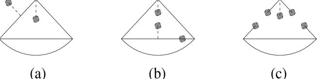
FIG. 2.: Dimension-4 power corrections: local (a,b) and bilocal (c). Shaded circles mark vacuum fields

The next term in OPE comes from dimension-four vacuum condensates. Diagrams from Fig. 2a,b are found to contribute,

$$-{1\over 144\pi^{2}p^{2}}\langle{\alpha_{s}\over\pi}F^{2}\rangle\left(\ln{-p^{2}\over\mu^{2}}+{7\over 6}+\ln{\mu^{2}\over-q^{2}}\right)\ ,$$ (16)

where $q^{2}$ is an infrared regulator which represents the momentum flow through the operator ${\cal O}^{\alpha}$. The infrared logarithm arises from large separations of point $z$ from $0$ and $x$. To take into account the contribution in this region properly, one must first expand the product of the interpolating current,

$$T\eta(x)\bar{\eta}(0)=\sum_{n}C_{n}(x)\hat{O}_{n}\ ,$$ (17)

(where $\hat{O}_{n}$ are a set of local operators) resulting in so-called bilocal power corrections [12] (see Fig. 2c). The relavant local operator in this case is a dimension-five one,

$$\hat{O}_{5}^{\lambda\rho\rho^{\prime}} = 2\bar{u}gF^{\lambda[\rho}\gamma^{\rho^{\prime}]}u-2i\partial^{[\rho}(\bar{u}\stackrel{{\scriptstyle\leftrightarrow}}{{D}}^{\lambda}\gamma^{\rho^{\prime}]}u)+\bar{u}\stackrel{{\scriptstyle\leftarrow}}{{\mathrel{\mathop{D\!\!\!/}}}}\stackrel{{\scriptstyle\rightarrow}}{{D}}^{\lambda}\sigma^{\rho\rho^{\prime}}u$$ (19)

$$+\bar{u}\sigma^{\rho\rho^{\prime}}\stackrel{{\scriptstyle\leftarrow}}{{D}}^{\lambda}\stackrel{{\scriptstyle\rightarrow}}{{\mathrel{\mathop{D\!\!\!/}}}}u+{3\over 4}\bar{u}gF^{\rho\rho^{\prime}}\gamma^{\lambda}u+{3\over 4}\bar{d}gF^{\rho\rho^{\prime}}\gamma^{\lambda}d\ ,$$

where $[\rho\rho^{\prime}]$ denotes antisymmetrization of the two indices. The operator yields a contribution to $W^{\mu\nu\alpha}$,

$$-{1\over 12\pi^{2}p^{2}}\Pi_{0}(0,\mu^{2})\ ,$$ (20)

where $\Pi_{0}(q^{2},\mu^{2})$ is a two-point correlation function between $\hat{O}_{5}^{\lambda\rho\rho^{\prime}}$ and ${\cal O}^{\alpha}$, and $\mu^{2}$ is an ultraviolet regulator to be defined below.

To calculate $\Pi_{0}(0,\mu^{2})$, we again use the sum rule approach. We first work out an operator-product expansion for $\Pi_{0}(q^{2})$ in the deep Euclidean space,

$$\Pi_{0}(q^{2},\mu^{2})={\alpha_{s}\over 60\pi^{3}}q^{4}\ln{\mu^{2}\over-q^{2}}+{1\over 12}\langle{\alpha_{s}\over\pi}F^{2}\rangle\ln{\mu^{2}\over-q^{2}}+{8\pi\alpha_{s}\over 9q^{2}}\langle\bar{u}u\rangle^{2}-{1\over 192\pi^{2}q^{2}}\langle g^{3}G^{3}\rangle+...$$ (21)

On the other hand, we write a dispersion integral for $\Pi_{0}(q^{2},\mu^{2})$ valid for all $q^{2}$ [14],

$$\Pi_{0}(q^{2},\mu^{2})={1\over\pi}\int^{\mu^{2}}_{0}{ds\over s}{\rho(s)-\rho_{\rm pert}(s)\over s-q^{2}}\ .$$ (22)

where the upper limit defines the ultraviolet cut-off and

$$\rho_{\rm pert}(s)={\alpha_{s}\over 60\pi^{2}}s^{3}\ .$$ (23)

$\Pi_{0}(q^{2})$ defined in this way vanishes in perturbation theory and its first power correction contributes in the same way as the last term in Eq. (16). To find $\Pi_{0}(0,\mu^{2})$, we assume a spectral function,

$$\rho(s)=\pi f_{R}m_{R}^{6}\delta(s-m_{R}^{2})+\theta(s-s_{0})\left({\alpha_{s}\over 60\pi^{2}}s^{3}+{\alpha_{s}\over 12}F^{2}s\right)$$ (24)

where $m_{R}$ is the mass scale for the exotic $1^{-+}$ resonace, suspected to lie between 1.3 to 1.9 GeV [13]. In our estimate, we take $m_{R}$ to be 1.5 MeV. The standard sum rule method allows us to extract $f_{R}$ = $1.8\times 10^{-3}$, which in turn yields $\Pi_{0}(0,m_{R}^{2})=5.0\times 10^{-4}m_{R}^{2}$. The uncertainty of this number is at least a factor of 2 due to unknown $m_{R}$ and the continuum threshold $s_{0}$, which we take to be $1.9^{2}$ GeV².

The next term in the OPE for $W^{\mu\nu\alpha}$ involves dimension-six vacuum condensates, for which we use the factorization assumption. A calculation of the diagrams in Fig. 3a,b,c (and similar ones which are not drawn)

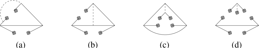
FIG. 3.: Typical local (a,b,c) and bilocal (d) power corrections of dimension 6.

give a contribution to $W^{\mu\nu\alpha}$,

$${\alpha_{s}\langle\bar{u}u\rangle^{2}\over 81\pi p^{4}}\left(20\ln{-p^{2}\over\mu^{2}}+62\ln{\mu^{2}\over-q^{2}}\right)\ ,$$ (25)

where we have kept only logarithmic terms. Small contribution of the first term to the final result justifies the approximation. The infrared logarithm in the second term signals that the contribution must be replaced by,

$${4\langle\bar{u}u\rangle\over 3p^{4}}\Pi_{1}(0,\mu^{2})\ ,$$ (26)

where $\Pi_{1}(q^{2},\mu^{2})$ is a bilocal correlator (see Fig 3d) give involving $\hat{\cal O}^{\alpha}$ and the dimension-seven operator,

$$\hat{O}_{7}^{\lambda\rho\rho^{\prime}}=\epsilon^{ijk}\epsilon^{i^{\prime}j^{\prime}k}(D^{\lambda}u)^{i}C\gamma^{\rho}u^{j}~{}\bar{u}^{j^{\prime}}\gamma^{\rho^{\prime}}C\bar{u}^{i^{\prime}T}+{\it h.c.}$$ (27)

The OPE for $\Pi_{1}(q^{2},\mu^{2})$ at large Euclidean $q^{2}$ is,

$$\Pi_{1}(q^{2})={31\over 54}{\alpha_{s}\over\pi}\langle\bar{u}u\rangle\ln{\mu^{2}\over-q^{2}}-{m_{0}^{2}\langle\bar{u}u\rangle\over 3q^{2}}+...$$ (28)

where $m_{0}^{2}=-\langle\bar{u}gF\cdot\sigma u\rangle/\langle\bar{u}u\rangle$. The higher-order terms in ellipese involve condensates of dimension-seven and higher for which we know very little. To get an estimate, we assume vector-meson dominace [15],

$$\Pi_{1}(q^{2})={f_{R}^{\prime}\over m^{2}_{R}-q^{2}}\ .$$ (29)

Expand the above in $q^{2}$ and matching its $1/q^{2}$ term with the OPE in Eq. (28), we find,

$$\Pi_{1}(0)={m_{0}^{2}\langle\bar{u}u\rangle\over 3m_{R}^{2}}\ .$$ (30)

We ignore dimension-eight or higher contributions. In the factorization approximation, the contributions from dimension-eight condensates (both local and bilocal) are exactly zero.

Based on the OPE we have developed for $W^{\mu\nu\alpha}$, we attempt an estimate for the $J_{g}(m_{N}^{2})$. The sum rule equation reads like this,

$${J_{g}\lambda^{2}\over(m_{N}^{2}-p^{2})^{2}}+... = {\alpha_{s}\over\pi^{5}}({1\over 144}\ln^{2}{-p^{2}\over\mu^{2}}-{1\over 36}\ln{-p^{2}\over\mu^{2}})p^{2}-{1\over 144\pi^{2}p^{2}}\langle{\alpha_{s}\over\pi}F^{2}\rangle\left(\ln{-p^{2}\over\mu^{2}}+{7\over 6}\right)$$ (32)

$$-{1.1\times 10^{-3}\over 12\pi^{2}p^{2}}+{20\alpha_{s}\over 81\pi}{\langle\bar{u}u\rangle^{2}\over p^{4}}\ln{-p^{2}\over\mu^{2}}+{4m_{0}^{2}\langle\bar{u}u\rangle^{2}\over 9m_{R}^{2}p^{4}}$$

Substituting in the standard values for the condenstates at the normalization pont $\mu=1GeV$ (ccf ref. [16] for example): $\langle(\alpha_{s}/\pi)F^{2}\rangle=0.012~{}{\rm GeV}^{4}$, $\langle\bar{u}u\rangle=-0.017~{}{\rm GeV}^{3}$, $m_{0}^{2}=0.65$, $\alpha_{s}(1~{}{\rm GeV})=0.37$, $32\pi^{4}\lambda_{N}^{2}=2.5~{}{\rm GeV}^{6}$, $s_{0}=2.25~{}{\rm GeV}^{2}$, we find that the dimension-six bilocal term is the dominant contribution. If we keep just this term, we find

$$J_{g}(1~{}{\rm GeV}^{2})={8em_{0}^{2}\langle\bar{u}u\rangle^{2}\over 9m_{R}^{2}\lambda^{2}_{N}}=0.25\ .$$ (33)

A more careful analysis including other contributions yields,

$$J_{g}(1~{}{\rm GeV}^{2})=0.35\pm 0.13\ .$$ (34)

where the error reflects the uncertainty of the mass scale in the $1^{-+}$ channel as well as the uncertainty from the sum rule analysis. However, we have no way to know the accuracy of the vector meson approximation in estimating the dimension-six bilocal contribution.

The number we find, $J_{g}(1~{}{\rm GeV}^{2})\sim 0.35\pm 0.13$ or $J_{q}(1~{}{\rm GeV}^{2})\sim 0.15\pm 0.13$, if taking seriously, has interesting implication on the spin structure of the nucleon. It says that gluons are at least as important in determining the nucleon spin as quarks, if not more. Furthermore, from a recent globle analysis of data on polarized deep-inelastic scattering[9], one finds the gluon helicity $\Delta G(1~{}{\rm GeV}^{2})$ defined in the infinite momentum frame and light-like gauge has a size of 1 to 2 units of angular momentum. If correct, the gluon orbital contribution defined in a similar framework must be large and negative and cancel a substential part of $\Delta G$. Such a large cancellation may be caused by the gauge-dependent separation of $J_{g}$ into helicity and orbital contributions. On the other hand, one half of the singlet-axial charge, or the quark spin contribution, is found to be $0.05^{+0.08}_{-0.05}$[9]. This leaves about 20% of the nucleon spin carried by quark orbital angular momentum. Here no large cancellation is present between the quark spin and orbital contributions.

REFERENCES

• [1] J. Ashman et al., Nucl. Phys. B328, 1 (1989).
• [2] For a review, see H. Y. Cheng, Int. J. Mod. Phys. A11, 5109 (1996); also, R. L. Jaffe, MIT-CTP-2518, Jan. 1996, hep-ph/9603422.
• [3] R. L. Jaffe and A. Manohar, Nucl. Phys. B337, 509 (1990).
• [4] V. Hughes et al., Proceeding of the 12th International Symposium on High-Energy Spin Physics, Amsterdam, Holland, Sept. 1996.
• [5] M. A. Shifman, A. I. Vainshtein, and V. I. Zakharov, Nucl. Phys. B147, 385, 448 (1979).
• [6] X. Ji, Phys. Rev. Lett. 78, 610 (1997); see also hep-ph/9609381.
• [7] A. V. Kolesnichenko, Sov. J. Nucl. Phys. 39, 968 (1984).
• [8] V. M. Belyaev and B. I. Blok, Z. Phys. C30, 279 (1986).
• [9] G. Altarelli, R. Ball, S. Forte, G. Ridolfi, hep-ph/9710289; R. D. Ball, S. Forte, and G. Ridolfi, Nucl. Phys. B444, 287 (1995).
• [10] X. Ji, J. Tang, and P. Hoodbhoy, Phys. Rev. Lett. 76, 740 (1996).
• [11] B. Ioffe, Z. Phys. C18, 67 (1983).
• [12] I. I. Balitsky, Phys. Lett. 114B, 53 (1983).
• [13] I. I. Balitsky, D. I. Dyakonov, and A. V. Yung, Z. Phys. C33, 265 (1986); N. Isgur and R. Kokoski, and J. Paton, Phys. Rev. Lett. 54, 869 (1985).
• [14] I. I. Balitsky, A. V. Kolesnichenko, and A. V. Yung, Sov. J. Nucl. Phys. 41, 178 (1985).
• [15] I. I. Balitsky and A. V. Yung, Phys. Lett. 129B, 328 (1983).
• [16] I. I. Balitsky, V.M. Braun, and A. V. Kolesnichenko, Phys. Lett. 242B, 245 (1990).