Cutting rules in the real time formalisms
at finite temperature

In this paper, we review the set of rules specific to the calculation of the imaginary part of a Green’s function at finite temperature in the real-time formalisms. Emphasis is put on the clarification of a recent controversy concerning these rules in the “$1/2$” formalism, more precisely on the issue related to the interpretation of these rules in terms of cut diagrams, like at $T=0$. On the second hand, new results are presented, enabling one to calculate the imaginary part of thermal Green’s functions in other formulations of the real-time formalism, like the “retarded/advanced” formalism in which a lot of simplifications occur.

ENSLAPP–A–639/97

hep-ph/9701410

1 Introduction

A long time ago, Kobes and Semenoff (KS in the following) presented in a series of two papers a generalization of the well known Cutkosky’s rules in order to calculate the imaginary part of a Green’s function in the Real Time Formalism (RTF) at finite temperature. In the first paper [1], they generalized in a straightforward way the rules valid at zero temperature for each term of the sum over the type $1$ or $2$ for the internal vertices of the diagram. This first step resulted in a huge number of terms to be evaluated in order to calculate the imaginary part of a diagram at finite temperature. In their second paper [2], they focused on thermal Green’s functions whose external points are all of type $1$, because in these days it was strongly believed that the type $1$ fields were “physical”, whereas the type $2$ fields were supposed to be “ghost fields” that could not appear on the external lines of a physical amplitude. For this kind of Green’s functions, the rules obtained in their first paper can be simplified considerably, but their conclusion is that the standard interpretation of these rules in terms of cut diagrams do not survive the thermalization. Naïvely, the reason of that difference between the $T=0$ and the $T\not=0$ cases lies in the fact that at $T=0$, a cut propagator, proportional to $\theta(\pm k_{0})$, imposes a definite sign to the energy flow, whereas at $T\not=0$, it is proportional to $\theta(\pm k_{0})\pm n_{{}_{B,F}}(|k_{0}|)$ so that the energy flow is not constrained any longer.

Recently, Bedaque, Das and Naik (BDN) claimed [3] that the interpretation in terms of cut diagrams holds also at finite temperature, despite the apparent lack of energy flow constraints in the high temperature cut propagators. Their proof is essentially based on the Kubo-Martin-Schwinger (KMS) identities verified by the high temperature Green’s functions, which imply a cancelation of the terms that do not correspond to a cut trough the diagram when performing the sum over the types $1$ or $2$ of the internal vertices. It is also obvious that such a cancelation is quite impossible in KS’s rules, since this sum is already performed by these rules. Moreover, a lot of actual calculations have been carried with the rules of KS, and contradictions with the results provided by other methods, like calculating the whole diagram and then taking the imaginary part or calculating the same quantity in the imaginary time formalism, have never been found, indicating that KS’s rules should be true despite their lack of interpretation in terms of cut diagrams. Nevertheless, BDN never explained in their paper the reason of the discrepancy between their result and KS’s result.

For these reasons, it seems useful to investigate the precise connections between the two approaches, in order to explain carefully the origin of their apparent discrepancy. This is the purpose of the section 2. The outline of that section is as follows: first, we recall the common starting point of both methods, which is a direct generalization of the $T=0$ Cutkosky’s rules. Then, we reproduce the derivation of KS’s rules, explaining how terms that does not correspond to cut diagrams arise, and why they are necessary in this approach. In the paragraph 2.3, we expose an abbreviated version of BDN’s proof, leading to a set of cutting rules in which every term is interpretable as a cut diagram. Finally, we explain where the apparent contradiction lies and compare the efficiency of both methods on an explicit example.

The section 3 is devoted to the presentation of the cutting rules that must be used in other versions of the real-time formalism. Indeed, Aurenche and Becherrawy [4], followed by van Eijck and van Weert [5], first presented a new set of Feynman rules that can be obtained trough a “rotation” applied to the usual “1/2” formalism. The aim of that transformation is to obtain a matrix propagator with two vanishing components, and without statistical factors. The statistical weights are then rejected into the vertices. The two non-vanishing components are nothing but the retarded and advanced zero-temperature propagators, which is at the origin of the denomination of this formalism as “Retarded/Advanced” (R/A) formalism. Then, van Eijck, Kobes and van Weert generalized that kind of transformations in [6]. The “R/A” formalism appeared to be only a particular example of this kind of transformations. In particular, two other formulations of the RTF appeared to be quite simple: the Keldysh formalism which is useful in problems related to the linear response theory, and the “Feynman/Anti Feynman” ($F$/$\bar{F}$) formalism which have also only two non-vanishing propagator components, which are the usual zero-temperature Feynman propagator and its complex conjugate.

The “R/A” formalism then proved to be quite efficient for carrying actual calculations [7], and to have very close connections with the imaginary time formalism [8, 9]. This is the reason why it would be very useful to have some rules enabling one to calculate the imaginary part of a Green’s function directly in the “R/A” formalism, and more generally in all the formalisms of [6]. This will be done quite simply in the section 3, first in the case of general transformations for which the “rotation” matrix is real, and then in the particular cases that correspond to the three formalisms evocated above. The “R/A” cutting rules appear to be very simple, and lead to quite compact calculations. Some emphasis will be put in the calculation of the imaginary part of self-energy diagrams, since this quantity is related to the decay rate and production rate of the external particle. In that particular case, the “R/A” cutting rules become even more simple.

Finally, section 4 is devoted to a summary and to concluding remarks.

2 Various approaches in the “$1/2$” formalism

2.1 Common starting point

We follow here the method which has been derived first by KS in [1]. In the $1/2$ formalism, every Green’s function with external points of types $a_{i}=1,2$ can be formally written as the sum over the types $1$ or $2$ of the internal vertices $v_{i}$:

$$G^{\{a_{i}\}}(\{k_{i}\})=\sum\limits_{\{v_{i}=1,2\}}G^{\{a_{i}\}\{v_{i}\}}(\{k_{i}\})\;,$$ (1)

where $G^{\{a_{i}\}\{v_{i}\}}(\{k_{i}\})$ is the term with external points of fixed type $a_{i}$ and internal vertices of type $v_{i}$. Then, taking the imaginary part:

$${\rm Im}\left(iG^{\{a_{i}\}}(\{k_{i}\})\right)=\sum\limits_{\{v_{i}=1,2\}}{\rm Im}\left(iG^{\{a_{i}\}\{v_{i}\}}(\{k_{i}\})\right)\;.$$ (2)

The first step towards the rules enabling to perform directly the calculation of this imaginary part is common to both KS and BDN approaches. It consists essentially in reproducing what is done at $T=0$ for each term of the sum of Eq. (2) and is based on the largest time equation. Following [1], we are led to introduce two kind of vertices; the usual ones

$$g^{1}=-ig,\;g^{2}=+ig\;,$$ (3)

and a set of “circled” vertices (represented by a small circle in the figures, and with an underlined label in the equations)

$$g^{\underline{1}}=+ig,\;g^{\underline{2}}=-ig\;,$$ (4)

which are nothing but the complex conjugates of the standard ones. Of course, we need also all the propagators enabling one to connect every pair of vertices. The usual thermal propagator $G^{ab}(k)$ is the propagator connecting an uncircled vertex of type $a$ to an uncircled vertex of type $b$, the momentum flow being $k$ in the direction $a\to b$:

$$G^{ab}(k)=\pmatrix{G^{11}(k)&G^{12}(k)\cr G^{21}(k)&G^{22}(k)\cr}\;,$$ (5)

the explicit expressions of these propagators being (for a contour parameter chosen to be $\sigma=0$) for bosonic fields:

$$G^{11}(k)=i{\cal P}\left({1\over{k^{2}-m^{2}}}\right)+\pi(1+2n_{{}_{B}}(|k_{0}|))\delta(k^{2}-m^{2})$$ (6)

$$G^{22}(k)=-i{\cal P}\left({1\over{k^{2}-m^{2}}}\right)+\pi(1+2n_{{}_{B}}(|k_{0}|))\delta(k^{2}-m^{2})$$ (7)

$$G^{12}(k)=2\pi(\theta(-k_{0})+n_{{}_{B}}(|k_{0}|))\delta(k^{2}-m^{2})$$ (8)

$$G^{21}(k)=2\pi(\theta(k_{0})+n_{{}_{B}}(|k_{0}|))\delta(k^{2}-m^{2})\;.$$ (9)

The propagators $G^{\underline{a}b}(k)$ connecting the circled vertex of type $a$ to the uncircled vertex of type $b$ and carrying the momentum $k$ are related to the standard ones by:

$$G^{\underline{a}b}(k)=\pmatrix{G^{12}(k)&G^{12}(k)\cr G^{21}(k)&G^{21}(k)\cr}\;.$$ (10)

With now obvious notations, we have also:

$$G^{a\underline{b}}(k)=\pmatrix{G^{21}(k)&G^{12}(k)\cr G^{21}(k)&G^{12}(k)\cr}\;$$ (11)

and

$$G^{\underline{a}\underline{b}}(k)=\pmatrix{G^{22}(k)&G^{12}(k)\cr G^{21}(k)&G^{11}(k)\cr}\;.$$ (12)

Then, following [1, 3], we obtain:

$${\rm Im}\left(iG^{\{a_{i}\}\{v_{i}\}}\right)(\{k_{i}\})=-{1\over 2}\sum\limits_{(\{a_{i}\}\{v_{i}\})}G^{(\{a_{i}\}\{v_{i}\})}(\{k_{i}\})\;,$$ (13)

where $\sum_{(\{a_{i}\}\{v_{i}\})}$ is a sum running over all the possibilities of circling the points $a_{i}$ and $v_{i}$, excepted the two terms where all or none of the points are circled, and $G^{(\{a_{i}\}\{v_{i}\})}(\{k_{i}\})$ is the corresponding term. In some sense, this formula is a simple generalization of the standard $T=0$ Cutkosky’s formula. The only difference lies of course in the fact that at $T=0$, one can further simplify the calculation of the imaginary part since the energy flow constraints induced by the propagators connecting circled to uncircled vertices (called “cut propagators” in the following) eliminates all the configurations of circles that do not correspond to a cut trough the diagram. As already mentioned, this appears to be impossible at high $T$ since the “cut propagators” do not constrain the energy flow at non vanishing $T$. Adding now the sum over the types of the internal vertices, we get for the imaginary part of the complete Green’s function:

$${\rm Im}\left(iG^{\{a_{i}\}}(\{k_{i}\})\right)=-{1\over 2}\sum\limits_{\{v_{i}=1,2\}}\sum\limits_{(\{a_{i}\}\{v_{i}\})}G^{(\{a_{i}\}\{v_{i}\})}(\{k_{i}\})\;.$$ (14)

This formula is the common starting point of KS and BDN approaches. It is important to notice that the number of terms to be evaluated in the right hand side of this equation is quite huge. Indeed, not only the sum over the types $1$ or $2$ of all the internal vertices is to be performed, but also the sum over the possibilities of circling vertices, without excluding the circlings that do not correspond to a cut diagram.

2.2 Kobes and Semenoff approach

At that point, KS managed in [2] to get rid of the sum $\sum_{\{v_{i}=1,2\}}$ to obtain a simpler expression of the imaginary part in the case where all the external points are of type $1$. The reason for such a choice was based on the common belief according to which the “physical fields” were of type $1$, whereas the type $2$ fields were “ghost fields”. Any physical amplitude therefore should have only type $1$ external points. Nowadays, this interpretation of type $1$ or $2$ fields has been ruled out by the fact that it is not clear what a “physical amplitude” at finite $T$ is (for instance, the most physically relevant self-energy function is not $\Sigma^{11}$ but the function which appears in the pole shift, as can be seen by performing a Dyson summation). Nevertheless, in the case of self-energies, the imaginary part of the relevant self-energy is related to the imaginary part of $\Sigma^{11}$ in a simple way (see [2]), so that the calculation of ${\rm Im}(\Sigma^{11})$ is sufficient.

In their final formula, there are only type $1$ external points and internal vertices:

$${\rm Im}\left(iG^{\{a_{i}=1\}}(\{k_{i}\})\right)=-{1\over 2}\sum\limits_{{(\{a_{i}=1\})}\atop{[\{v_{i}=1\}]}}G^{(\{a_{i}=1\}),[\{v_{i}=1\}]}(\{k_{i}\})\;,$$ (15)

where the sum $\sum_{{(\{a_{i}=1\})}\atop{[\{v_{i}=1\}]}}$ runs over all the possibilities of circling the external points $a_{i}$ excepted the two terms where all or none of them are circled, and all the possibilities of circling the internal vertices $v_{i}$. The important advantage compared to Eq. (14) lies in the fact that the sum over the type of the internal vertices is already performed, which reduces drastically the number of terms to be evaluated. A very simple proof of that formula can also be found in [10].

This formula leads to some difficulties in its interpretation since it generates some terms that does not correspond to cuts through the diagram, i.e. to topologies where the “cut propagators” (propagators connecting a circled to an uncircled vertex) do not divide the diagram in two connected parts. two examples of such a contributions are reproduced in Fig. 1. One should note that in this approach, there is a complete equivalence between the cut propagators and the “on-shell” propagators, i.e. propagators that are proportional to a factor $\delta(k^{2}-m^{2})$. Moreover, it should be emphazised that these “uncut terms” are necessary in this formula in order to have the cancelation of the pathologies consisting in products of distributions having overlapping supports, like $\delta^{2}(k^{2}-m^{2})$ or $({\cal P}(1/(k^{2}-m^{2})))^{2}$: without these terms, the result would be ill-defined. This is what happens for the first example of Fig. 1. But, it would not be consistent to simply drop these “uncut terms”, by arguing that they are here only for the cancelation of pathologies, because that these “uncut terms” can occur even when there are no pathologies to be canceled, like in the second diagram of Fig. 1.

So, the conclusion of this approach is that despite a considerable reduction of the number of terms, the formula Eq. (15) generates unavoidably a few terms that are not interpretable in terms of cut diagrams, these terms being absolutely necessary for the completeness of the result.

2.3 Bedaque, Das and Naik approach

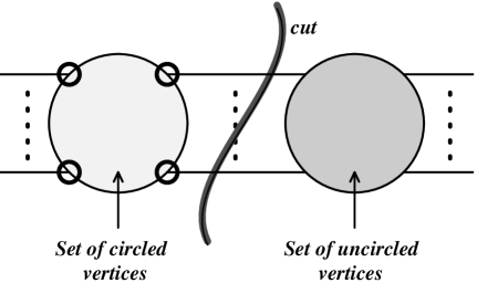
Figure 2: Structure of a cut diagram in the approach of Bedaque, Das and Naik.

After formula (14), BDN took an orthogonal way compared to KS, since they chose to reduce the number of terms contained in that formula by trying to simplify the sum $\sum_{(\{a_{i}\}\{v_{i}\})}$ while keeping the sum $\sum_{\{v_{i}=1,2\}}$ unchanged. In their approach, there is no need of a special assumption concerning the type $1$ or $2$ of the external points of the diagram. In fact, they proved that the effect of the sum $\sum_{\{v_{i}=1,2\}}$ was to kill all the configurations of circlings that do not correspond to cut diagrams, a cut diagram being generically of the type depicted in Fig. 2. Of course, in the remaining terms, the sum $\sum_{\{v_{i}=1,2\}}$ is still to be performed.

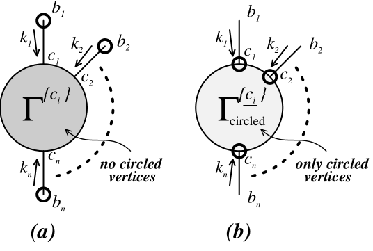
Figure 3: Terms that are canceled by the summation over the type $1$ or $2$ of the internal vertices.

In what follows, we give a simple proof of that result. Let us first notice that it is enough to prove that the configurations where a set of uncircled vertices is completely surrounded by circled vertices only (and vice versa) are killed by the sum over the type of the $v_{i}$’s. These configurations occur when the disposition of the circles in the diagram is such that the diagram contains a subdiagram of one of the types depicted in Fig. 3. In the figure 3, the vertices labeled by $c_{i}$ are obviously internal, so that we must sum over the types $c_{i}=1,2$. It is this sum that will make these configurations vanish.

Let us begin by the configuration of Fig. 3-(a). The corresponding terms in the right hand side of Eq. (14) are proportional to the quantity:

$$F^{\{\underline{b_{i}}\}}(\{k_{i}\})\equiv\sum\limits_{\{c_{i}=1,2\}}\Gamma^{\{c_{i}\}}(\{k_{i}\})\,\prod\limits_{i=1}^{n}G^{\underline{b_{i}}c_{i}}(k_{i})\;,$$ (16)

where $\Gamma^{\{c_{i}\}}(\{k_{i}\})$ is the $n$-point vertex function with external points $c_{i}$ and entering momenta $k_{i}$ (the signs associated to type $c_{i}=2$ external vertices are included in its definition). Looking at the propagators connecting a circled vertex to an uncircled one in Eq. (10), we obtain:

$$F^{\{\underline{b_{i}}\}}(\{k_{i}\})=\prod\limits_{\{i|b_{i}=1\}}G^{12}(k_{i})\prod\limits_{\{i|b_{i}=2\}}G^{21}(k_{i})\sum\limits_{\{c_{i}=1,2\}}\Gamma^{\{c_{i}\}}(\{k_{i}\})=0\;,$$ (17)

since the $n$-point vertex functions satisfy the identity [11, 12]:

$$\sum\limits_{\{c_{i}=1,2\}}\Gamma^{\{c_{i}\}}(\{k_{i}\})=0\;.$$ (18)

This identity is in fact the Fourier expression of the largest time equation used in [1]. It is worth noticing that this cancelation survives in an out-of-equilibrium field theory since this identity is always verified.

Considering now the configuration of Fig. 3-(b), the corresponding terms in the right hand side of Eq. (14) are proportional to:

$$F^{\{b_{i}\}}(\{k_{i}\})\equiv\sum\limits_{\{c_{i}=1,2\}}\Gamma^{\{\underline{c_{i}}\}}_{\rm circled}(\{k_{i}\})\,\prod\limits_{i=1}^{n}G^{b_{i}\underline{c_{i}}}(k_{i})\;,$$ (19)

where $\Gamma^{\{\underline{c_{i}}\}}_{\rm circled}(\{k_{i}\})$ is the $n$-point vertex function made only of circled vertices. Therefore, this vertex function is nothing but the complex conjugate of the previous one:

$$\Gamma^{\{\underline{c_{i}}\}}_{\rm circled}(\{k_{i}\})=\left(\Gamma^{\{c_{i}\}}(\{k_{i}\})\right)^{*}\;.$$ (20)

Making use of Eq. (11), we can write:

$$\halign to=0.0pt{\@eqnsel\hskip\@centering$\displaystyle{#}$&\global\@eqcnt\@ne\hskip 2\arraycolsep\hfil${#}$\hfil&\global\@eqcnt\tw@\hskip 2\arraycolsep$\displaystyle{#}$\hfil&\llap{#}\cr 0.0pt plus 1000.0pt$\displaystyle{F^{\{b_{i}\}}(\{k_{i}\})&10.0pt\hfil${&10.0pt$\displaystyle{=\sum\limits_{\{c_{i}=1,2\}} \left( \Gamma^{\{c_{i}\}}(\{k_{i}\})\right)^{*} \prod\limits_{\{i|c_{i}=1\}} G^{21}(k_{i}) \prod\limits_{\{i|c_{i}=2\}} G^{12}(k_{i})\\ &\hbox to0.0pt{\hss&=\left[\prod\limits_{i=1}^{n}2\pi(\theta(k_{i}^{0})+n_{{}_{B}}(|k_{i}^{0}|))\delta(k_{i}^{2}-m_{i}^{2})\right]\;\sum\limits_{\{c_{i}=1,2\}}\left(\prod\limits_{\{i|c_{i}=2\}}e^{-\beta k_{i}^{0}}\right)\left(\Gamma^{\{c_{i}\}}(\{k_{i}\})\right)^{*}\\&&=0\;,&(21)\cr}}}}}$$

the last equality being a consequence of the identity [11, 12]:

$$\sum\limits_{\{c_{i}=1,2\}}\left(\prod\limits_{\{i|c_{i}=2\}}e^{-\beta k_{i}^{0}}\right)\Gamma^{\{c_{i}\}}(\{k_{i}\})=0\;,$$ (22)

which is nothing but the expression of the Kubo-Martin-Schwinger property for $n$-point real time vertex functions. This relation was used by [2] in time coordinates where it appears to be related to the $-i\beta$ periodicity properties of Green’s functions. One can note that this cancelation is not true in an out-of-equilibrium plasma since it makes use of the KMS relations which are specific to thermal equilibrium.

Therefore, taking these cancelations into account, we can reduce the sum $\sum_{(\{a_{i}\}\{v_{i}\})}$ over the disposition of circles to a smaller sum where we keep only those terms that correspond to a cut through the diagram, like on Fig. 2. We can then write:

$${\rm Im}\left(iG^{\{a_{i}\}}(\{k_{i}\})\right)=-{1\over 2}\sum\limits_{\{v_{i}=1,2\}}\sum\limits_{\rm cuts}G^{(\{a_{i}\}\{v_{i}\})}(\{k_{i}\})\;.$$ (23)

In that formula, the sum over the type $1$ or $2$ of the internal vertices $v_{i}$ is still to be performed for the remaining terms. This fact happens to generate more terms than with the final formula of Kobes and Semenoff. The issue of the efficiency of both methods will be discussed on an example in the next paragraph.

One could then wonder why it is possible thanks to the KMS relations to eliminate the same configurations of circles than at $T=0$, despite the the fact that apparently these relations have nothing to do with energy flow constraints. In fact, the study of the $T=0$ limit of the KMS relations of Eq. (22) indicates that the KMS identity appears to be a thermal generalization of some energy flow constraints. Indeed, it is possible to show that a direct consequence of Eq. (22) is:

$$\lim_{T\to 0^{+}}\Gamma^{\{c_{i}\}}(\{k_{i}\})\propto\theta\left(\sum\limits_{\{i|c_{i}=2\}}k_{i}^{0}\right)\;.$$ (24)

A proof of this relation is given in the appendix. So, even if this limit is not a proof of the fact that KMS should play at positive $T$ the same role than energy flow constraints at $T=0$, it points towards the interpretation of the KMS identity as the thermal generalization of a very simple constraint on energy flow.

2.4 Are the two methods contradictory ?

Let us first explain where lies the apparent contradiction between the conclusions of KS and BDN concerning the issue of the interpretation in terms of cut diagrams:

• In Eq. (15), some terms are not interpretable as the contribution of a cut diagram. Moreover, as already said, the uncut propagators can only be $G^{11}(k)$ or $G^{\underline{1}\underline{1}}(k)=G^{22}(k)$. It means that the uncut propagators are always off-shell (i.e. not proportional to a Dirac delta function). On the contrary, all the cut propagators are on-shell.

• In Eq. (23), all the terms are interpretable as contributions of cut diagrams. Moreover, with the same definition as in KS approach for a cut propagator (i.e. connecting the circled vertices to the uncircled ones), the uncut propagators in this approach can be any of $G^{ab}(k)$ or $G^{\underline{a}\underline{b}}(k)$. Among them, we find $G^{12}(k)$ and $G^{21}(k)$ which are on-shell. This is an essential difference with the approach of KS.

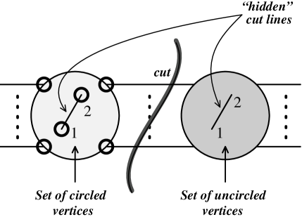
Figure 4: “Hidden” cuts in the terms generated in the approach of Bedaque, Das and Naik.

Therefore, the expression “cut propagator” does not cover the same reality in both approaches. Some of the uncut propagators (more precisely, those which are on-shell) of BDN are considered to be cut ones in KS method. It means that more propagators are called “cut propagators” in KS’s approach than in BDN’s one, and this is of course at the origin of the apparent discrepancy. Naïvely speaking, if one has more “cut propagators”, then it will be difficult to have only configurations where the set of cut propagators form a single cut through the diagram. This assertion is illustrated in the figure 4, in which we see clearly how some of the cut propagators of KS, spoiling the interpretation of the imaginary part in terms of cut diagrams, are “hidden” in the approach of BDN.

Now, in order to be more explicit, let us consider in detail the example of the diagram of Fig. 1 for the theory of a real scalar field. If we use the method of KS to compute the contribution of this topology to the imaginary part of $\Sigma^{11}(k)$, we must evaluate the $8$ terms represented on Fig. 5. After some straightforward calculations, we get for the contribution of the individual terms (actually, we grouped them by pairs since some terms differ only by a factor $e^{-\beta q^{0}}$, as proven in [2]):

$${\rm Im}^{{}^{KS}}_{(1+5)}(\Sigma^{11}(q))= {{(1+e^{-\beta q^{0}})}\over{2}}\int{{d^{4}r}\over{(2\pi)^{4}}}\;G^{21}(p)\left[{{(1+e^{\beta r^{0}})\sigma^{21}(r)+e^{\beta r^{0}}\sigma^{22}(r)}\over{e^{\beta r^{0}}-1}}\right]$$ (30)

$$\times\left\{2i\pi^{2}{{e^{\beta r^{0}}+1}\over{e^{\beta r^{0}}-1}}\delta^{2}(r^{2}-m^{2})+\pi\epsilon(r^{0})\delta^{\prime}(r^{2}-m^{2})\right\}\;,$$

$${\rm Im}^{{}^{KS}}_{(2+6)}(\Sigma^{11}(q))= -{{(1+e^{-\beta q^{0}})}\over{2}}\int{{d^{4}r}\over{(2\pi)^{4}}}\;G^{21}(p)\sigma^{21}(r)$$ (31)

$$\times\left\{2i\pi^{2}{{e^{2\beta r^{0}}+1}\over{(e^{\beta r^{0}}-1)^{2}}}\delta^{2}(r^{2}-m^{2})+i{\cal P}{1\over{(r^{2}-m^{2})^{2}}}\right\}\;,$$

$${\rm Im}^{{}^{KS}}_{(3+7)}(\Sigma^{11}(q))= {{(1+e^{-\beta q^{0}})}\over{2}}\int{{d^{4}r}\over{(2\pi)^{4}}}\;{{e^{\beta r^{0}}G^{21}(p)\sigma^{22}(r)}\over{e^{\beta r^{0}}-1}}$$ (32)

$$\times\left\{-2i\pi^{2}{{e^{\beta r^{0}}+1}\over{e^{\beta r^{0}}-1}}\delta^{2}(r^{2}-m^{2})+\pi\epsilon(r^{0})\delta^{\prime}(r^{2}-m^{2})\right\}\;,$$

$${\rm and}$$

$${\rm Im}^{{}^{KS}}_{(4+8)}(\Sigma^{11}(q))= -{{(1+e^{-\beta q^{0}})}\over{2}}\int{{d^{4}r}\over{(2\pi)^{4}}}\;{{e^{\beta r^{0}}G^{21}(p)\sigma^{21}(r)}\over{(e^{\beta r^{0}}-1)^{2}}}4i\pi^{2}\delta^{2}(r^{2}-m^{2})\;,$$ (33)

where the $\sigma^{ij}(r)$ are components of the one-loop self-energy matrix. It is instructive to note that the cancelation of the pathologic products of distributions occur only when all the terms are added, and not at the level of the individual terms. Adding all these contributions, we finally get:

$$\halign to=0.0pt{\@eqnsel\hskip\@centering$\displaystyle{#}$&\global\@eqcnt\@ne\hskip 2\arraycolsep\hfil${#}$\hfil&\global\@eqcnt\tw@\hskip 2\arraycolsep$\displaystyle{#}$\hfil&\llap{#}\cr 0.0pt plus 1000.0pt$\displaystyle{{\rm Im}^{{}^{KS}}_{(1+\cdots+8)}(\Sigma^{11}(q))=&10.0pt\hfil${&10.0pt$\displaystyle{{{(1+e^{-\beta q^{0}})}\over{2}} \int{{d^{4}r}\over{(2\pi)^{4}}}\; G^{21}(p)\left\{-i\sigma^{21}(r){\cal P}{1\over{(r^{2}-m^{2})^{2}}}\right.\\ &\hbox to0.0pt{\hss&\left.+\pi\left[{{2e^{\beta r^{0}}\sigma^{22}(r)+(1+e^{\beta r^{0}})\sigma^{21}(r)}\over{e^{\beta r^{0}}-1}}\right]\epsilon(r^{0})\delta^{\prime}(r^{2}-m^{2})\right\}\;.&(34)\cr}}}}}$$

For the same quantity, the method of BDN requires the calculation of the $6\times 4=24$ terms of Fig. 6. For each disposition of the circles, the calculations are heavier than in the KS’s method since one should perform the sum over $a,b=1,2$. Here again, we can group the terms by pairs:

$${\rm Im}^{{}^{BDN}}_{(1+6)}(\Sigma^{11}(q))= -{{(1+e^{-\beta q^{0}})}\over{2}}\int{{d^{4}r}\over{(2\pi)^{4}}}\;G^{21}(p)\left[{{e^{\beta r^{0}}\sigma^{22}(r)+\sigma^{21}(r)}\over{e^{\beta r^{0}}-1}}\right]$$ (35)

$$\times\left\{2i\pi^{2}\delta^{2}(r^{2}-m^{2})-\pi\epsilon(r^{0})\delta^{\prime}(r^{2}-m^{2})\right\}\;,$$

$${\rm Im}^{{}^{BDN}}_{(2+5)}(\Sigma^{11}(q))= -{{(1+e^{-\beta q^{0}})}\over{2}}\int{{d^{4}r}\over{(2\pi)^{4}}}\;G^{21}(p)\sigma^{21}(p)$$ (36)

$$\times\left\{2i\pi^{2}\delta^{2}(r^{2}-m^{2})+i{\cal P}{1\over{(r^{2}-m^{2})^{2}}}\right\}\;,$$

$${\rm and}$$

$${\rm Im}^{{}^{BDN}}_{(3+4)}(\Sigma^{11}(q))= {{(1+e^{-\beta q^{0}})}\over{2}}\int{{d^{4}r}\over{(2\pi)^{4}}}\;G^{21}(p)\left[{{e^{\beta r^{0}}(\sigma^{22}(r)+\sigma^{21}(r))}\over{e^{\beta r^{0}}-1}}\right]$$ (37)

$$\times\left\{2i\pi^{2}\delta^{2}(r^{2}-m^{2})+\pi\epsilon(r^{0})\delta^{\prime}(r^{2}-m^{2})\right\}\;.$$

Of course, the sum of all the contributions is the same as the one obtained previously in Eq (2.4). Here again, we note that if we sum only groups of terms that correspond to the same cut, we obtain expressions that are not defined by themselves. This seems to indicate that, even if in the approach of Bedaque, Das and Naik the interpretation in terms of cut diagrams survives, the interpretation of the terms obtained as products of physical amplitudes is meaningless since these terms are ill-defined when considered alone. This conclusion is different from that of BDN, but this discrepancy is simply related to the fact that they never considered in [3] explicit examples where pathologies do arise.

To conclude this section, one can say that the methods provided by KS and BDN are not in contradiction despite the appearances; that KS’s method leads to simpler calculations; and that, contrary to the claim of BDN, the decomposition provided by Eq. (23) is not completely consistent with an interpretation in terms of the underlying physical amplitudes.

3 About the other bases of the real-time formalism

3.1 General considerations

We follow here the approach of [6] in order to define new formulations of the real time formalism, initially expressed in the $1/2$ base. The general aim of this method is to derive formalisms in which the constraints provided by the relations of Eq. (18) and Eq. (22) correspond to the nullity of certain components of the new $n$-point vertex functions, instead of the nullity of complicated linear combinations. Another practical advantage lies in the fact that for some of these modified formalisms the statistical weights are rejected into the vertices, which clarify the calculations.

Let us define new Green’s functions by the transformation:

$${\tenimbf G}^{\{X_{i}\}}(\{k_{i}\})\equiv\sum\limits_{\{a_{i}=1,2\}}G^{\{a_{i}\}}(\{k_{i}\})\prod\limits_{i=1}^{n}U^{X_{i}a_{i}}(k_{i})\;,$$ (38)

with an invertible “rotation matrix” $U^{Xa}(k)$ so that the reverse transformation exists. The new index $X$ takes also two distinct values, and will be denoted by capital letters. Before going further, it is useful to slightly modify the notations for the vertices in the $1/2$ formalism. Instead of $g^{1}$ and $g^{2}$, we introduce $8$ vertices $g^{abc}$, so that $g^{111}=-g^{222}=-ig$ whereas all the other components are vanishing. By doing so, at each vertex, we have to perform the sum $\sum_{\{a,b,c=1,2\}}g^{abc}$. In the new formalism, the vertex functions should be defined so that holds the relation:

$$\sum\limits_{\{X_{i}\}}{\tenimbf\Gamma}^{\{X_{i}\}}(\{k_{i}\})\prod\limits_{i=1}^{n}{\tenimbf G}^{Y_{i}X_{i}}(k_{i})=\sum\limits_{\{a_{i}=1,2\}}\sum\limits_{\{b_{i}=1,2\}}\Gamma^{\{b_{i}\}}(\{k_{i}\})\prod\limits_{i=1}^{n}U^{Y_{i}a_{i}}(k_{i})G^{a_{i}b_{i}}(k_{i})\;,$$ (39)

in order to be consistent with the definition chosen for complete Green’s functions. By multiplication of the above equation by the appropriate inverse propagators, this requirement leads one to:

$${\tenimbf\Gamma}^{\{X_{i}\}}(\{k_{i}\})=\sum\limits_{\{a_{i}=1,2\}}\Gamma^{\{a_{i}\}}(\{k_{i}\})\prod\limits_{i=1}^{n}V^{X_{i}a_{i}}(k_{i})\;,$$ (40)

where we defined

$$V^{Xa}(k)\equiv\left((U^{{}^{T}})^{-1}\right)^{Xa}(-k)\;.$$ (41)

Now, in order to be able to say something about the imaginary part of the transformed Green’s functions, we limit ourselves to those transformations for which the rotation matrix $U(k)$ is real. With such a restriction, we have:

$${\rm Im}\left(i{\tenimbf G}^{\{X_{i}\}}(\{k_{i}\})\right)=\sum\limits_{\{a_{i}=1,2\}}{\rm Im}\left(iG^{\{a_{i}\}}(\{k_{i}\})\right)\prod\limits_{i=1}^{n}U^{X_{i}a_{i}}(k_{i})\;.$$ (42)

Then, we reproduce the usual way of justifying the Feynman’s rules in the transformed formalism, which consists in writing each object (propagator, vertex) belonging to the $1/2$ formalism in the right hand side of Eq. (38) as a function of its counterpart in the rotated formalism. Then, the rotation matrices cancel by pairs $UU^{-1}$ when linking propagators to vertices. If we apply this procedure to the circling rules obtained in the “$1/2$” formalism for the calculation of ${\rm Im}\left(G^{\{a_{i}\}}\right)$, we obtain analogous circling rules in the transformed formalism. For this, it is necessary to define, in complete analogy with the definition of the transformed propagators and vertices, the counterparts of $G^{\underline{a}b}$, $G^{a\underline{b}}$, $G^{\underline{a}\underline{b}}$ and $g^{\underline{a}\underline{b}\underline{c}}$. This gives:

$${\tenimbf G}^{\underline{X}Y}(k)=\sum\limits_{\{a,b=1,2\}}U^{Xa}(k)U^{Yb}(-k)G^{\underline{a}b}(k)$$ (43)

$${\tenimbf G}^{X\underline{Y}}(k)=\sum\limits_{\{a,b=1,2\}}U^{Xa}(k)U^{Yb}(-k)G^{a\underline{b}}(k)$$ (44)

$${\tenimbf G}^{\underline{X}\underline{Y}}(k)=\sum\limits_{\{a,b=1,2\}}U^{Xa}(k)U^{Yb}(-k)G^{\underline{a}\underline{b}}(k)$$ (45)

for the propagators, and:

$$\halign to=0.0pt{\@eqnsel\hskip\@centering$\displaystyle{#}$&\global\@eqcnt\@ne\hskip 2\arraycolsep\hfil${#}$\hfil&\global\@eqcnt\tw@\hskip 2\arraycolsep$\displaystyle{#}$\hfil&\llap{#}\cr 0.0pt plus 1000.0pt$\displaystyle{{\tenimbf g}^{\text@underline{XYZ}}(k_{1},k_{2},k_{3})&10.0pt\hfil${&10.0pt$\displaystyle{=\sum\limits_{\{a,b,c=1,2\}} V^{Xa}(k_{1}) V^{Yb}(k_{2}) V^{Zc}(k_{3}) g^{\text@underline{abc}}\\ &\hbox to0.0pt{\hss&=-{\tenimbf g}^{XYZ}(k_{1},k_{2},k_{3})&(46)\cr}}}}}$$

for the vertex. If we denote by $\alpha$ and $\bar{\alpha}$ the two values taken by the index $X$ in the new formalism, the analogue of Eq. (14) is:

$${\rm Im}\left({\tenimbf G}^{\{X_{i}\}}(\{k_{i}\})\right)=-{1\over 2}\sum\limits_{\{V_{i}=\alpha\alpha\alpha,\alpha\alpha\bar{\alpha},\cdots\}}\;\sum\limits_{(\{X_{i}\}\{V_{i}\})}{\tenimbf G}^{(\{X_{i}\}\{V_{i}\})}(\{k_{i}\})\;,$$ (47)

where the sum $\sum_{\{V_{i}=\alpha\alpha\alpha,\alpha\alpha,\bar{\alpha},\cdots\}}$ is the sum over the possible types of the internal vertices $V_{i}$, and the sum $\sum_{(\{X_{i}\}\{V_{i}\})}$ runs over all the possibilities of circling external points and vertices, excepted the two terms where all or none of them are circled.

Here also, it is possible to eliminate from the sum all the terms that do not correspond to a cut diagram. To do so, we need first to obtain the relations that correspond in the new formalism to the constraints provided by Eq. (18) and Eq. (22). Let us first invert the relation Eq. (40), which gives:

$$\Gamma^{\{a_{i}\}}(\{k_{i}\})=\sum\limits_{\{X_{i}=\alpha,\bar{\alpha}\}}{\tenimbf\Gamma}^{\{X_{i}\}}(\{k_{i}\})\prod\limits_{i=1}^{n}\left(U^{{}^{T}}\right)^{a_{i}X_{i}}(-k_{i})\;.$$ (48)

Then, it is trivial to obtain the relation that corresponds to Eq. (18) in the new formalism

$$\sum\limits_{\{X_{i}=\alpha,\bar{\alpha}\}}\left(\sum\limits_{\{a_{i}=1,2\}}\prod\limits_{i=1}^{n}\left(U^{{}^{T}}\right)^{a_{i}X_{i}}(-k_{i})\right){\tenimbf\Gamma}^{\{X_{i}\}}(\{k_{i}\})=0\;,$$ (49)

and for the KMS relation Eq. (22):

$$\sum\limits_{\{X_{i}=\alpha,\bar{\alpha}\}}\left(\sum\limits_{\{a_{i}=1,2\}}\prod\limits_{\{i|a_{i}=2\}}e^{-\beta k_{i}^{0}}\prod\limits_{i=1}^{n}\left(U^{{}^{T}}\right)^{a_{i}X_{i}}(-k_{i})\right){\tenimbf\Gamma}^{\{X_{i}\}}(\{k_{i}\})=0\;.$$ (50)

To see if the configurations analogous to that of Fig. 3-(a) do cancel in the sum, we are lead to the evaluation of

$$\halign to=0.0pt{\@eqnsel\hskip\@centering$\displaystyle{#}$&\global\@eqcnt\@ne\hskip 2\arraycolsep\hfil${#}$\hfil&\global\@eqcnt\tw@\hskip 2\arraycolsep$\displaystyle{#}$\hfil&\llap{#}\cr 0.0pt plus 1000.0pt$\displaystyle{{\tenimbf F}^{\{\text@underline{X_{i}}\}}(\{k_{i}\})&10.0pt\hfil${&10.0pt$\displaystyle{\equiv\sum\limits_{\{Y_{i}=\alpha,\bar{\alpha}\}} {\tenimbf\Gamma}^{\{Y_{i}\}}(\{k_{i}\}) \prod\limits_{i=1}^{n} {\tenimbf G}^{\text@underline{X_{i}}Y_{i}}(k_{i})\\ &\hbox to0.0pt{\hss&=\sum\limits_{\{a_{i}=1,2\}}\prod\limits_{\{i|a_{i}=1\}}G^{12}(k_{i})\prod\limits_{\{i|a_{i}=2\}}G^{21}(k_{i})\prod\limits_{i=1}^{n}U^{X_{i}a_{i}}(k_{i})\\&&\quad\times\sum\limits_{\{Y_{i}=\alpha,\bar{\alpha}\}}\left(\sum\limits_{\{b_{i}=1,2\}}\prod\limits_{i=1}^{n}\left(U^{{}^{T}}\right)^{b_{i}Y_{i}}(-k_{i})\right){\tenimbf\Gamma}^{\{Y_{i}\}}(\{k_{i}\})\\&&=0\;,&(51)\cr}}}}}$$

thanks to Eq. (49). This cancelation survives in out-of-equilibrium theories since it is based only on the generalization to the new formalism of an identity which is always true. For the configuration of circles of Fig. 3-(b), we must now evaluate:

$$\halign to=0.0pt{\@eqnsel\hskip\@centering$\displaystyle{#}$&\global\@eqcnt\@ne\hskip 2\arraycolsep\hfil${#}$\hfil&\global\@eqcnt\tw@\hskip 2\arraycolsep$\displaystyle{#}$\hfil&\llap{#}\cr 0.0pt plus 1000.0pt$\displaystyle{{\tenimbf F}^{\{X_{i}\}}(\{k_{i}\})&10.0pt\hfil${&10.0pt$\displaystyle{\equiv\sum\limits_{\{Y_{i}=\alpha,\bar{\alpha}\}} {\tenimbf\Gamma}^{\{\text@underline{Y_{i}}\}}_{\rm circled}(\{k_{i}\}) \prod\limits_{i=1}^{n} {\tenimbf G}^{X_{i}\text@underline{Y_{i}}}(k_{i})\\ &\hbox to0.0pt{\hss&=\sum\limits_{\{a_{i}=1,2\}}\prod\limits_{i=1}^{n}2\pi(\theta(k_{i}^{0})+n_{{}_{B}}(|k_{i}^{0}|))\delta(k_{i}^{2}-m_{i}^{2})U^{X_{i}a_{i}}(k_{i})\\&&\quad\times\sum\limits_{\{Y_{i}=\alpha,\bar{\alpha}\}}\left(\sum\limits_{\{b_{i}=1,2\}}\prod\limits_{\{i|b_{i}=2\}}e^{-\beta k_{i}^{0}}\prod\limits_{i=1}^{n}\left(U^{{}^{T}}\right)^{b_{i}Y_{i}}(-k_{i})\right)\left({\tenimbf\Gamma}^{\{Y_{i}\}}(\{k_{i}\})\right)^{*}\\&&=0\;,&(52)\cr}}}}}$$

due to Eq. (50). Therefore, the same configurations of circles can be eliminated from the sum giving the imaginary part of the Green’s function in any formalism obtained by Eq. (38). As a consequence, we can generalize in any such formalism the formula of BDN:

$${\rm Im}\left({\tenimbf G}^{\{X_{i}\}}\right)(\{k_{i}\})=-{1\over 2}\sum\limits_{\{V_{i}=\alpha\alpha\alpha,\alpha\alpha\bar{\alpha},\cdots\}}\sum\limits_{\rm cuts}{\tenimbf G}^{(\{X_{i}\}\{V_{i}\})}(\{k_{i}\})\;.$$ (53)

In the following paragraphs, we specialize to three particular such formalisms, that are the Keldysh formalism, the “$F/\bar{F}$” formalism and the “R/A” formalism.

3.2 The Keldysh basis

The aim of the transformation leading to this formalism is to use the relation Eq. (18) in order to make one component of the matrix propagator vanish. Since this identity is true even in out-of-equilibrium theories, this formalism can be applied without modifications in such a case.

A “rotation matrix” leading to that is:

$$U(k)={1\over{\sqrt{2}b(-k^{0})}}\pmatrix{&b(k^{0})b(-k^{0})&b(k^{0})b(-k^{0})\cr&+1&-1\cr}\;,$$ (54)

where $b(k^{0})$ is an arbitrary function of $k^{0}$, non vanishing at $k^{0}=0$. In this paragraph, we denote by $+$ the label of the first row , and by $-$ the label of the second one. Performing such a transformation, we get for the propagators:

$${\tenimbf G}^{XY}(k)=\pmatrix{&b(k^{0})b(-k^{0})(G^{12}(k)+G^{21}(k))&G^{11}(k)-G^{12}(k)\cr&G^{11}(k)-G^{21}(k)&0\cr}\;,$$ (55)

$${\tenimbf G}^{\underline{X}Y}(k)=\pmatrix{&b(k^{0})b(-k^{0})(G^{12}(k)+G^{21}(k))&0\cr&G^{12}(k)-G^{21}(k)&0\cr}\;,$$ (56)

$${\tenimbf G}^{X\underline{Y}}(k)=\pmatrix{&b(k^{0})b(-k^{0})(G^{12}(k)+G^{21}(k))&G^{21}(k)-G^{12}(k)\cr&0&0\cr}\;,$$ (57)

$${\rm and}$$

$${\tenimbf G}^{\underline{XY}}(k)=\pmatrix{&b(k^{0})b(-k^{0})(G^{12}(k)+G^{21}(k))&G^{21}(k)-G^{11}(k)\cr&G^{12}(k)-G^{11}(k)&0\cr}\;.$$ (58)

As announced, the standard propagator ${\tenimbf G}^{XY}(k)$ possesses a vanishing component. We see also that the propagators connecting circled to uncircled vertices have two vanishing components. Despite these zeros, the simplifications one could expect in the calculations based on this formalism are almost compensated by the fact that the vertices are more intricate than in the $``1/2"$ formalism. Indeed, one obtains for the vertices:

$${{{\tenimbf g}^{X_{1}X_{2}X_{3}}(k_{1},k_{2},k_{3})}\over{-ig}}={{1-(-1)^{\#\{i|X_{i}=-\}}}\over{2^{3/2}}}\prod\limits_{\{i|X_{i}=+\}}{1\over{b(-k_{i}^{0})}}\prod\limits_{\{i|X_{i}=-\}}b(k_{i}^{0})\;,$$ (59)

where $\#\{i|X_{i}=-\}$ stands for the number of indices equal to $-$. It appears that the function $b(k^{0})$, which remained unspecified until now, can simply be chosen to equal $b(k^{0})=1$.

On can note that the extra-diagonal terms of the matrix propagator in the Keldysh formalism are nothing but retarded and advanced zero-temperature propagators:

$$G^{11}(k)-G^{12}(k)=\Delta_{{}_{R}}(k)\equiv i{\cal P}{1\over{k^{2}-m^{2}}}+\pi\epsilon(k_{0})\delta(k^{2}-m^{2})$$ (60)

$$G^{11}(k)-G^{21}(k)=\Delta_{{}_{A}}(k)\equiv i{\cal P}{1\over{k^{2}-m^{2}}}-\pi\epsilon(k_{0})\delta(k^{2}-m^{2})\;.$$ (61)

For $n$-point functions, ${\tenimbf G}^{+-\cdots-}(\{k_{i}\})$ is a $n$-point retarded function. More generally, the Green’s functions in the Keldysh formalism can be interpreted as response functions in the linear response theory.

At that point, the formula we get for the calculation of the imaginary part of a Green’s function expressed in the Keldysh basis is, in analogy with Eq. (14):

$${\rm Im}\left({\tenimbf G}^{\{X_{i}\}}(\{k_{i}\})\right)=-{1\over 2}\sum\limits_{\{V_{i}=+++,++-,\cdots\}}\;\sum\limits_{(\{X_{i}\}\{V_{i}\})}{\tenimbf G}^{(\{X_{i}\}\{V_{i}\})}(\{k_{i}\})\;,$$ (62)

where $\sum_{\{V_{i}=+++,++-,\cdots\}}$ is the sum over the possible types of the internal vertices $V_{i}$, and the sum $\sum_{(\{X_{i}\}\{V_{i}\})}$ runs over all the possibilities of circling external points and vertices, excepted the two terms where all or none of them are circled.

If we remain in the general case of an out-of-equilibrium field theory, the result of BDN cannot be generalized in totality because the KMS identity is not true. More precisely, the configurations of Fig. 3-(a) can be removed from the sum, thanks to the identity Eq. (49) which takes here a very simple form:

$${\tenimbf\Gamma}^{\{+\cdots+\}}(\{k_{i}\})=0\;.$$ (63)

But in the general case the configurations of Fig. 3-(b) cannot. To remove them also, one must restrict to an equilibrium theory, so that holds the relation Eq. (50), which takes here the form:

$$\sum\limits_{\{X_{i}=\pm\}}{\tenimbf\Gamma}^{\{X_{i}\}}(\{k_{i}\})\prod\limits_{\{i|X_{i}=+\}}b(k^{0})b(-k^{0})(1+e^{-\beta k_{i}^{0}})\prod\limits_{\{i|X_{i}=-\}}(1-e^{-\beta k_{i}^{0}})=0\;.$$ (64)

If thermal equilibrium holds, then we have only configurations of circles that correspond to cuts through the diagram:

$${\rm Im}\left({\tenimbf G}^{\{X_{i}\}}\right)(\{k_{i}\})=-{1\over 2}\sum\limits_{\{V_{i}=+++,++-,\cdots\}}\sum\limits_{\rm cuts}{\tenimbf G}^{(\{X_{i}\}\{V_{i}\})}(\{k_{i}\})\;.$$ (65)

3.3 The $F/\bar{F}$ basis

3.3.1 Cutting rules in the “$F/\bar{F}$” formalism

In this formalism, one implements also the KMS relation of Eq. (22) in order to make a second component of the matrix propagator vanish. There are more than one possibility to achieve that. In one of them, we obtain for the non vanishing components the usual zero-temperature Feynman propagator and its complex conjugate. Of course, since the statistical factors have disappeared in the propagator, the new vertices must contain the information relative to the temperature.

A transformation enabling this for bosons is generated by the following $U$ matrix:

$$\halign to=0.0pt{\@eqnsel\hskip\@centering$\displaystyle{#}$&\global\@eqcnt\@ne\hskip 2\arraycolsep\hfil${#}$\hfil&\global\@eqcnt\tw@\hskip 2\arraycolsep$\displaystyle{#}$\hfil&\llap{#}\cr 0.0pt plus 1000.0pt$\displaystyle{U(k)=&10.0pt\hfil${&10.0pt$\displaystyle{\theta(k^{0})\pmatrix{&c(k^{0}) &- e^{-\beta k^{0}} c(k^{0})\cr&- d(k^{0}) &d(k^{0})\cr}\\ &\hbox to0.0pt{\hss&\quad+\theta(-k^{0}){{n_{{}_{B}}(-k^{0})e^{-\beta k^{0}}}\over{c(-k^{0})d(-k^{0})}}\pmatrix{&d(-k^{0})&-d(-k^{0})\cr&-e^{\beta k^{0}}c(-k^{0})&c(-k^{0})\cr}\;,&(66)\cr}}}}}$$

where $c(k^{0})$ and $d(k^{0})$ are arbitrary functions of the energy, non vanishing at the point $k^{0}=0$.

Performing this transformation, we obtain:

$${\tenimbf G}^{XY}(k)=\pmatrix{&\Delta_{{}_{F}}(k)&0\cr&0&\Delta_{{}_{\bar{F}}}(k)\cr}\;,$$ (67)

$${\tenimbf G}^{\underline{X}Y}(k)=\pmatrix{&2\pi\theta(-k^{0})\delta(k^{2}-m^{2})&0\cr&0&2\pi\theta(k^{0})\delta(k^{2}-m^{2})\cr}\;,$$ (68)

$${\tenimbf G}^{X\underline{Y}}(k)=\pmatrix{&2\pi\theta(k^{0})\delta(k^{2}-m^{2})&0\cr&0&2\pi\theta(-k^{0})\delta(k^{2}-m^{2})\cr}\;,$$ (69)

$${\rm and}$$

$${\tenimbf G}^{\underline{XY}}(k)=\pmatrix{&\Delta_{{}_{\bar{F}}}(k)&0\cr&0&\Delta_{{}_{F}}(k)\cr}\;,$$ (70)

where we defined

$$\Delta_{{}_{F}}(k)\equiv i{\cal P}{1\over{k^{2}-m^{2}}}+\pi\delta(k^{2}-m^{2})$$ (71)

$$\Delta_{{}_{\bar{F}}}(k)\equiv-i{\cal P}{1\over{k^{2}-m^{2}}}+\pi\delta(k^{2}-m^{2})\;.$$ (72)

Here again, the difficulty in using this formalism for practical calculations lies in the complexity of the vertices:

$$\halign to=0.0pt{\@eqnsel\hskip\@centering$\displaystyle{#}$&\global\@eqcnt\@ne\hskip 2\arraycolsep\hfil${#}$\hfil&\global\@eqcnt\tw@\hskip 2\arraycolsep$\displaystyle{#}$\hfil&\llap{#}\cr 0.0pt plus 1000.0pt$\displaystyle{&10.0pt\hfil${&10.0pt$\displaystyle{{{{\tenimbf g}^{X_{1}X_{2}X_{3}}(k_{1},k_{2},k_{3})}\over{-ig}}\\ &\hbox to0.0pt{\hss&\qquad=\prod\limits_{\{i|X_{i}=F\}}\left[\theta(k_{i}^{0})c(k_{i}^{0})+\theta(-k_{i}^{0}){{e^{-\beta k_{i}^{0}}n_{{}_{B}}(-k_{i}^{0})}\over{c(-k_{i}^{0})}}\right]\prod\limits_{\{i|X_{i}=\bar{F}\}}\left[\theta(k_{i}^{0})d(k_{i}^{0})+\theta(-k_{i}^{0}){{n_{{}_{B}}(-k_{i}^{0})}\over{d(-k_{i}^{0})}}\right]\\&&\quad-\prod\limits_{\{i|X_{i}=F\}}\left[\theta(k_{i}^{0})c(k_{i}^{0})+\theta(-k_{i}^{0}){{n_{{}_{B}}(-k_{i}^{0})}\over{c(-k_{i}^{0})}}\right]\prod\limits_{\{i|X_{i}=\bar{F}\}}\left[\theta(k_{i}^{0})e^{\beta k_{i}^{0}}d(k_{i}^{0})+\theta(-k_{i}^{0}){{n_{{}_{B}}(-k_{i}^{0})}\over{d(-k_{i}^{0})}}\right]\;.&(73)\cr}}}}}$$

In particular, there is no simple choice of the functions $c(k^{0})$ and $d(k^{0})$ enabling one to simplify significantly these vertices. In this particular formalism, the constraints provided by the relations Eq. (49) and Eq. (50) are:

$$\sum\limits_{\{X_{i}=F,\bar{F}\}}{\tenimbf\Gamma}^{\{X_{i}\}}(\{k_{i}\})\prod\limits_{\{i|X_{i}=F\}}\theta(-k_{i}^{0})c(-k_{i}^{0})(1-e^{\beta k_{i}^{0}})\prod\limits_{\{i|X_{i}=\bar{F}\}}{{\theta(k_{i}^{0})}\over{d(k_{i}^{0})}}=0\;,$$ (74)

and

$$\sum\limits_{\{X_{i}=F,\bar{F}\}}{\tenimbf\Gamma}^{\{X_{i}\}}(\{k_{i}\})\prod\limits_{\{i|X_{i}=F\}}{{\theta(k_{i}^{0})}\over{c(k_{i}^{0})}}\prod\limits_{\{i|X_{i}=\bar{F}\}}\theta(-k_{i}^{0})d(-k_{i}^{0})(e^{-\beta k_{i}^{0}}-1)=0\;.$$ (75)

If we are at thermal equilibrium, both of them are true, and the imaginary part of a “$F/\bar{F}$” Green’s function is given by:

$${\rm Im}\left({\tenimbf G}^{\{X_{i}\}}\right)(\{k_{i}\})=-{1\over 2}\sum\limits_{\{V_{i}=FFF,FF\bar{F},\cdots\}}\sum\limits_{\rm cuts}{\tenimbf G}^{(\{X_{i}\}\{V_{i}\})}(\{k_{i}\})\;.$$ (76)

3.4 Non-equilibrium “$F/\bar{F}$” formalism

Since the derivation of the propagators of this formalism makes an explicit use of the KMS relation, the “$F/\bar{F}$” cannot be generalized to non equilibrium situations without changes. For example, the propagators we get by the transformation Eq. (3.3.1) without using the KMS relation are:

$$\!\!\!\!\!\!\!\!\!\!\!\!{\tenimbf G}^{XY}(k)=\pmatrix{&G^{11}(k)-\theta(k^{0})G^{12}(k)-\theta(-k^{0})G^{21}(k)\!\!\!\!\!\!\!\!\!\!\!\!&\theta(k^{0})\Theta(k)\displaystyle{{c(k^{0})}\over{d(k^{0})}}\cr&\theta(-k^{0})\Theta(-k)\displaystyle{{c(-k^{0})}\over{d(-k^{0})}}&\!\!\!\!\!\!\!\!\!\!\!\!\theta(k^{0})G^{21}(k)+\theta(-k^{0})G^{12}(k)-G^{11}(k)\cr}\;,$$ (77)

$$\!\!\!\!\!\!\!\!\!\!\!\!{\tenimbf G}^{\underline{X}Y}(k)=\pmatrix{&\theta(-k^{0})(G^{12}(k)-G^{21}(k))&\theta(k^{0})\Theta(k)\displaystyle{{c(k^{0})}\over{d(k^{0})}}\cr&\theta(-k^{0})\Theta(-k)\displaystyle{{c(-k^{0})}\over{d(-k^{0})}}&\theta(k^{0})(G^{21}(k)-G^{12}(k))\cr}\;,$$ (78)

$$\!\!\!\!\!\!\!\!\!\!\!\!{\tenimbf G}^{X\underline{Y}}(k)=\pmatrix{&\theta(k^{0})(G^{21}(k)-G^{12}(k))&\theta(k^{0})\Theta(k)\displaystyle{{c(k^{0})}\over{d(k^{0})}}\cr&\theta(-k^{0})\Theta(-k)\displaystyle{{c(-k^{0})}\over{d(-k^{0})}}&\theta(-k^{0})(G^{12}(k)-G^{21}(k))\cr}\;,$$ (79)

$$\!\!\!\!\!\!\!\!\!\!\!\!{\rm and}$$

$$\!\!\!\!\!\!\!\!\!\!\!\!{\tenimbf G}^{\underline{XY}}(k)=\pmatrix{&\theta(k^{0})G^{21}(k)+\theta(-k^{0})G^{12}(k)-G^{11}(k)\!\!\!\!\!\!\!\!\!\!\!\!&\theta(k^{0})\Theta(k)\displaystyle{{c(k^{0})}\over{d(k^{0})}}\cr&\theta(-k^{0})\Theta(-k)\displaystyle{{c(-k^{0})}\over{d(-k^{0})}}&\!\!\!\!\!\!\!\!\!\!\!\!G^{11}(k)-\theta(k^{0})G^{12}(k)-\theta(-k^{0})G^{21}(k)\cr}\;,$$ (80)

where we denoted

$$\Theta(k)\equiv G^{12}(k)-e^{-\beta k^{0}}G^{21}(k)\;.$$ (81)

This quantity, vanishing at thermal equilibrium, quantifies how far we are from the equilibrium at the temperature $T$. We notice that the non-diagonal components are now non-vanishing (but remain small if we are close to equilibrium at temperature $T$), whereas the vertices remain the same, so that this formalism is not adapted to non equilibrium calculations. The reason why both of the non-diagonal components are non zero whereas we still use the first constraint Eq. (18) lies in the fact that the “$F/\bar{F}$” formalism does not implement the two constraints Eq. (18) and Eq. (22) individually, but rather implements two distinct linear combinations of these identities: therefore, both of these linear combinations are non zero if the KMS relation is not true anymore. Moreover, if we are out of equilibrium, the KMS relation Eq. (75) is not satisfied, and we must keep all the terms that contain configurations of circles of the type of Fig. 3-(b).

3.5 The $R/A$ basis

3.5.1 Cutting rules in the “R/A” formalism

The “R/A” formalism is of the same kind as the “$F/\bar{F}$” one since it implements the two constraints Eq. (18) and Eq. (22). It has therefore two vanishing components in its propagator. The difference lies in the nature of the non vanishing components, which are now the zero temperature retarded and advanced propagators. A transformation matrix that leads to that formalism for bosons is (the remarks made for the $F/\bar{F}$ formalism concerning fermions are also valid in this paragraph):

$$U(k)={1\over{a(-k^{0})}}\pmatrix{&a(k^{0})a(-k^{0})&-a(k^{0})a(-k^{0})\cr&-n_{{}_{B}}(-k^{0})&-n_{{}_{B}}(k^{0})\cr}\;,$$ (82)

where $a(k^{0})$ is an arbitrary function of $k^{0}$, non vanishing at $k^{0}=0$.

The propagators we obtain by this transformation are:

$${\tenimbf G}^{XY}(k)=\pmatrix{&0&\Delta_{{}_{A}}(k)\cr&\Delta_{{}_{R}}(k)&0\cr}\;,$$ (83)

$${\tenimbf G}^{\underline{X}Y}(k)=\pmatrix{&0&\Delta_{{}_{A}}(k)-\Delta_{{}_{R}}(k)\cr&0&0\cr}\;,$$ (84)

$${\tenimbf G}^{X\underline{Y}}(k)=\pmatrix{&0&0\cr&\Delta_{{}_{R}}(k)-\Delta_{{}_{A}}(k)&0\cr}\;,$$ (85)

$${\rm and}$$

$${\tenimbf G}^{\underline{XY}}(k)=\pmatrix{&0&-\Delta_{{}_{R}}(k)\cr&-\Delta_{{}_{A}}(k)&0\cr}\;.$$ (86)

As usual for such a transformation, the thermal information is now carried by the vertices:

$${{{\tenimbf g}^{X_{1}X_{2}X_{3}}(k_{1},k_{2},k_{3})}\over{-ig}}={{\prod\limits_{\{i|X_{i}=A\}}a(k_{i}^{0})}\over{\prod\limits_{\{i|X_{i}=R\}}a(-k_{i}^{0})}}\prod\limits_{\{i|X_{i}=R\}}n_{{}_{B}}(k_{i}^{0})\left[\prod\limits_{\{i|X_{i}=R\}}e^{\beta k_{i}^{0}}-1\right]\;.$$ (87)

To precise the vertices, we must make a choice for the function $a(k^{0})$. A convenient choice is $a(k^{0})=-n_{{}_{B}}(k^{0})$. With such a choice, we have for a vertex coupling three bosons:

$${\tenimbf g}^{{}^{AAA}}={\tenimbf g}^{{}^{RRR}}=0$$ (88)

$${\tenimbf g}^{{}^{ARR}}={\tenimbf g}^{{}^{RAR}}={\tenimbf g}^{{}^{RRA}}=-ig$$ (89)

$${\tenimbf g}^{{}^{RAA}}(k_{1},k_{2},k_{3})=ig(1+n_{{}_{B}}(k_{2}^{0})+n_{{}_{B}}(k_{3}^{0}))$$ (90)

$${\tenimbf g}^{{}^{ARA}}(k_{1},k_{2},k_{3})=ig(1+n_{{}_{B}}(k_{1}^{0})+n_{{}_{B}}(k_{3}^{0}))$$ (91)

$${\tenimbf g}^{{}^{AAR}}(k_{1},k_{2},k_{3})=ig(1+n_{{}_{B}}(k_{1}^{0})+n_{{}_{B}}(k_{2}^{0}))\;.$$ (92)

We note that the vertices with only advanced or only retarded labels are vanishing. This property is in fact general for any $n$-point Green’s function in the “R/A” formalism, since the constraints Eq. (49) and Eq. (50) are now:

$${\tenimbf\Gamma}^{\{R\cdots R\}}(\{k_{i}\})=0$$ (93)

$${\tenimbf\Gamma}^{\{A\cdots A\}}(\{k_{i}\})=0\;.$$ (94)

Thanks to these relations, the configurations of circles depicted in Fig. 3 both cancel in the calculation of the imaginary part, so that we are left with:

$${\rm Im}\left({\tenimbf G}^{\{X_{i}\}}\right)(\{k_{i}\})=-{1\over 2}\sum\limits_{\{V_{i}=RRA,RAR,\cdots\}}\sum\limits_{\rm cuts}{\tenimbf G}^{(\{X_{i}\}\{V_{i}\})}(\{k_{i}\})\;.$$ (95)

This formalism appears to be particularly simple for the application of cutting rules. Indeed, each matrix propagator have at least two vanishing components, and the propagators connecting circled vertices to uncircled ones even have three zero components. The presence of these zeros has the property to reduce considerably the number of terms left by the sum over the type of the internal vertices. Moreover, contrary to the “$F/\bar{F}$” formalism, the vertices remain rather simple.

3.5.2 Non-equilibrium “R/A” formalism

Again, some of the nice features of this formalism disappear when one does not use the KMS relation any longer. The propagators we are left with in such circumstances are:

$${\tenimbf G}^{XY}(k)=\pmatrix{&0&G^{11}(k)-G^{21}(k)\cr&G^{11}(k)-G^{12}(k)&\displaystyle{{e^{\beta k^{0}}\Theta(k)}\over{a(k^{0})a(-k^{0})(e^{\beta k^{0}}-1)}}\cr}\;,$$ (96)

$${\tenimbf G}^{\underline{X}Y}(k)=\pmatrix{&0&G^{12}(k)-G^{21}(k)\cr&0&\displaystyle{{e^{\beta k^{0}}\Theta(k)}\over{a(k^{0})a(-k^{0})(e^{\beta k^{0}}-1)}}\cr}\;,$$ (97)

$${\tenimbf G}^{X\underline{Y}}(k)=\pmatrix{&0&0\cr&G^{21}(k)-G^{12}(k)&\displaystyle{{e^{\beta k^{0}}\Theta(k)}\over{a(k^{0})a(-k^{0})(e^{\beta k^{0}}-1)}}\cr}\;,$$ (98)

$${\rm and}$$

$${\tenimbf G}^{\underline{XY}}(k)=\pmatrix{&0&G^{12}(k)-G^{11}(k)\cr&G^{21}(k)-G^{11}(k)&\displaystyle{{e^{\beta k^{0}}\Theta(k)}\over{a(k^{0})a(-k^{0})(e^{\beta k^{0}}-1)}}\cr}\;.$$ (99)

Compared to what happens out of equilibrium in the “$F/\bar{F}$” basis, we obtain at least one vanishing component and one component which is small if we consider a situation close to a thermal equilibrium at temperature $T$. Again, we have an extra zero component in the propagators connecting circled to uncircled vertices. Therefore, the “R/A” formalism appears to be the simplest one, even out of equilibrium.

3.6 The case of self-energies

3.6.1 Spectral representation of self-energies

Since the calculation of the imaginary part of two-point proper functions is of great importance when one is calculating production rates or decay rates of some particle, we devote a separate paragraph to the study of self-energies, having in mind the calculation of their imaginary part. Before going on, one should emphasize that in general, we are not interested in the self-energy expressed in a particular formalism, but rather in the function that enters the pole shift of a resummed propagator. In order to make the connection between this quantity and the self-energies in various formalisms, it is convenient to start with the spectral representation of two-point proper functions. This implies that we restrict ourselves to equilibrium theories since the KMS identity is required to derive the spectral representation of Green’s functions. Let us write it first in the “1/2” formalism, where it is well known (see for instance [12, 17]):

$$-i\Sigma^{11}(k_{0},{\tenimbf k})=\int\limits_{-\infty}^{+\infty}dE\;\sigma(E,{\tenimbf k})\,G^{11}(k_{0},E)\;,$$ (100)

$$-i\Sigma^{22}(k_{0},{\tenimbf k})=\int\limits_{-\infty}^{+\infty}dE\;\sigma(E,{\tenimbf k})\,G^{22}(k_{0},E)\;,$$ (101)

$$-i\Sigma^{12}(k_{0},{\tenimbf k})=-\int\limits_{-\infty}^{+\infty}dE\;\sigma(E,{\tenimbf k})\,G^{12}(k_{0},E)\;,$$ (102)

$$-i\Sigma^{21}(k_{0},{\tenimbf k})=-\int\limits_{-\infty}^{+\infty}dE\;\sigma(E,{\tenimbf k})\,G^{21}(k_{0},E)\;,$$ (103)

where $\sigma(E,{\tenimbf k})$ is a real function, and where $G^{ij}(k_{0},E)$ denotes the propagator $G^{ij}$ in which the on-shell energy $\omega_{k}\equiv\surd{({\tenimbf k}^{2}+m^{2})}$ has been replaced by $E$. The minus signs in the $12$ and $21$ components are due to the opposite sign of the type $2$ vertices. For later convenience, we can summarize these four relations by the single equation:

$$-i\Sigma^{ij}(k_{0},{\tenimbf k})=\int\limits_{-\infty}^{+\infty}dE\;\sigma(E,{\tenimbf k})\,\sum\limits_{\{k,l=1,2\}}\tau_{3}^{ik}\tau_{3}^{jl}G^{kl}(k_{0},E)\;,$$ (104)

where $\tau_{3}$ is the Pauli matrix along the $z$-direction. Using now the inverse of Eq. (38) and Eq. (40) in the case of $2$-point functions, we get:

$$-i{\tenimbf\Sigma}^{XY}(k)=\int\limits_{-\infty}^{+\infty}dE\;\sigma(E,{\tenimbf k})\,\sum\limits_{\{U,V=\alpha,\bar{\alpha}\}}W^{XU}(k)W^{YV}(-k){\tenimbf G}^{UV}(k_{0},E)\;,$$ (105)

where we defined

$$W^{XU}(k)\equiv\sum\limits_{\{i,k=1,2\}}V^{Xi}(k)\tau_{3}^{ik}\left(U^{-1}\right)^{kU}(k)\;.$$ (106)

For the Keldysh formalism, we obtain

$$W(k)=\pmatrix{&0&1\cr&1&0\cr}\;,$$ (107)

so that we have

$$-i{\tenimbf\Sigma}^{++}(k_{0},{\tenimbf k})=\int\limits_{-\infty}^{+\infty}dE\;\sigma(E,{\tenimbf k})\,{\tenimbf G}^{--}(k_{0},E)=0\;,$$ (108)

$$-i{\tenimbf\Sigma}^{--}(k_{0},{\tenimbf k})=\int\limits_{-\infty}^{+\infty}dE\;\sigma(E,{\tenimbf k})\,{\tenimbf G}^{++}(k_{0},E)\;,$$ (109)

$$-i{\tenimbf\Sigma}^{+-}(k_{0},{\tenimbf k})=\int\limits_{-\infty}^{+\infty}dE\;\sigma(E,{\tenimbf k})\,{\tenimbf G}^{-+}(k_{0},E)\;,$$ (110)

$${\rm and}$$

$$-i{\tenimbf\Sigma}^{-+}(k_{0},{\tenimbf k})=\int\limits_{-\infty}^{+\infty}dE\;\sigma(E,{\tenimbf k})\,{\tenimbf G}^{+-}(k_{0},E)\;.$$ (111)

In the case of the “$F/\bar{F}$” formalism, we get:

$$W(k)=\pmatrix{&1&0\cr&0&-1\cr}\;,$$ (112)

so that we have

$$-i{\tenimbf\Sigma}^{{}^{FF}}(k_{0},{\tenimbf k})=\int\limits_{-\infty}^{+\infty}dE\;\sigma(E,{\tenimbf k})\,{\tenimbf G}^{{}^{FF}}(k_{0},E)\;,$$ (113)

$$-i{\tenimbf\Sigma}^{{}^{\bar{F}\bar{F}}}(k_{0},{\tenimbf k})=\int\limits_{-\infty}^{+\infty}dE\;\sigma(E,{\tenimbf k})\,{\tenimbf G}^{{}^{\bar{F}\bar{F}}}(k_{0},E)\;,$$ (114)

$$-i{\tenimbf\Sigma}^{{}^{F\bar{F}}}(k_{0},{\tenimbf k})=-\int\limits_{-\infty}^{+\infty}dE\;\sigma(E,{\tenimbf k})\,{\tenimbf G}^{{}^{F\bar{F}}}(k_{0},E)=0\;,$$ (115)

$${\rm and}$$

$$-i{\tenimbf\Sigma}^{{}^{\bar{F}F}}(k_{0},{\tenimbf k})=-\int\limits_{-\infty}^{+\infty}dE\;\sigma(E,{\tenimbf k})\,{\tenimbf G}^{{}^{\bar{F}F}}(k_{0},E)=0\;.$$ (116)

Finally, for the “R/A” formalism, we have:

$$W(k)=\pmatrix{&0&1\cr&1&0\cr}\;,$$ (117)

which leads to

$$-i{\tenimbf\Sigma}^{{}^{RR}}(k_{0},{\tenimbf k})=\int\limits_{-\infty}^{+\infty}dE\;\sigma(E,{\tenimbf k})\,{\tenimbf G}^{{}^{AA}}(k_{0},E)=0\;,$$ (118)

$$-i{\tenimbf\Sigma}^{{}^{AA}}(k_{0},{\tenimbf k})=\int\limits_{-\infty}^{+\infty}dE\;\sigma(E,{\tenimbf k})\,{\tenimbf G}^{{}^{RR}}(k_{0},E)=0\;,$$ (119)

$$-i{\tenimbf\Sigma}^{{}^{RA}}(k_{0},{\tenimbf k})=\int\limits_{-\infty}^{+\infty}dE\;\sigma(E,{\tenimbf k})\,{\tenimbf G}^{{}^{AR}}(k_{0},E)\;,$$ (120)

$${\rm and}$$

$$-i{\tenimbf\Sigma}^{{}^{AR}}(k_{0},{\tenimbf k})=\int\limits_{-\infty}^{+\infty}dE\;\sigma(E,{\tenimbf k})\,{\tenimbf G}^{{}^{RA}}(k_{0},E)\;.$$ (121)

3.6.2 Imaginary part of self-energies in various formalisms

Then, thanks to these relations and to the fact that the spectral function $\sigma(E,{\tenimbf k})$ is the same in all the formalisms, we can relate the imaginary part of self-energies in various formalisms and choose the formalism that leads to the simplest calculations. In particular, we obtain for the imaginary part of the pole shift of the Feynman propagator:

$${\rm Im}\left({\tenimbf\Sigma}^{{}^{FF}}(k)\right) =\pi\int\limits_{-\infty}^{+\infty}dE\;\sigma(E,{\tenimbf k})\,\delta(k_{0}^{2}-E^{2})$$ (128)

$$={\rm Im}\left({\tenimbf\Sigma}^{{}^{\bar{F}\bar{F}}}(k)\right)$$

$$={{-i{\tenimbf\Sigma}^{--}(k)}\over{2b(k_{0})b(-k_{0})(1+2n_{{}_{B}}(|k_{0}|))}}$$

$$=\epsilon(k_{0}){\rm Im}\left({\tenimbf\Sigma}^{-+}(k)\right)=\epsilon(-k_{0}){\rm Im}\left({\tenimbf\Sigma}^{+-}(k)\right)$$

$$=\epsilon(k_{0}){\rm Im}\left({\tenimbf\Sigma}^{{}^{RA}}(k)\right)=\epsilon(-k_{0}){\rm Im}\left({\tenimbf\Sigma}^{{}^{AR}}(k)\right)$$

$$={{{\rm Im}\left(\Sigma^{11}(k)\right)}\over{1+2n_{{}_{B}}(|k_{0}|)}}={{{\rm Im}\left(\Sigma^{22}(k)\right)}\over{1+2n_{{}_{B}}(|k_{0}|)}}$$

$$={{i\Sigma^{12}(k)}\over{2(\theta(-k_{0})+n_{{}_{B}}(|k_{0}|))}}={{i\Sigma^{21}(k)}\over{2(\theta(k_{0})+n_{{}_{B}}(|k_{0}|))}}\;.$$

3.6.3 Calculation of self-energies in the “R/A” formalism

Practically, it appears that the “R/A” formalism leads to very compact calculations for the imaginary part of self-energies. In particular, looking at the place of the vanishing terms in the “R/A” matrix propagators, and using the concept of “$\epsilon$-flow” introduced in [9], we can prove the following statements:

• The connected set of uncircled vertices must be linked to the external leg on which enters the retarded momentum.

• The sum over the internal indices $R$ or $A$ contains a single non vanishing term if the cut goes through all the loops of the diagram (i.e. the configuration of the internal $R$ or $A$ indices is totally constrained by such a cut).

• If the cut is more general and keeps some loops uncut, it divides the diagram in two amplitudes, one of them being of the $AR\cdots R$ type while the other one is the complex conjugate of a $RA\cdots A$ amplitude. This is another proof of a result contained in [9]. Moreover, these amplitudes are quite simple analytic continuations from the imaginary time formalism. Nevertheless, as in the “1/2” cutting rules, the interpretation of the imaginary part as a sum of products of amplitudes is not completely meaningful since each of these products is not defined by itself due to pathologic products of distributions.

To conclude this paragraph, one can say that the “R/A” formalism appears to be quite simple to calculate imaginary parts of self-energies, because of the presence of many vanishing components in the propagators of this formalism. Moreover, the fact that it gives expressions in which the statistical weights are factorized in the vertices proves to be very helpful to clarify the calculations. The “R/A” formalism seems to be the only one for which BDN’s formula is more efficient than the “1/2” formalism used with the KS rules. For instance, in the case of the example already considered on Fig. 5, BDN’s formula in association with the “R/A” formalism leads to three terms, to be compared with the eight (only four in practice, since they can be combined by pairs differing only by a simple factor) terms generated by the method of KS.

4 Summary

The first result of this paper is to make a detailed comparison of two apparently contradictory approaches for the calculation of the imaginary part of thermal Green’s functions in the “1/2” real time formalism. It appeared that the two methods are in fact completely equivalent in the sense that they lead to the same result. Moreover, despite the fact that Bedaque, Das and Naik’s method seems to lead to a more common interpretation of the imaginary part in terms of products of amplitudes, this interpretation is partly spoiled by the fact that the terms that would correspond to such an interpretation are in fact ill-defined when considered individually. From the point of view of the length of the calculations, the method of Kobes and Semenoff appeared to be much more efficient.

The second part of the paper has been devoted to the generalization of the cutting rules already obtained in the “1/2” formalism, in order to give similar rules for other bases of the real time formalism. It appeared that such rules are in fact quite general, and that the result of Bedaque, Das and Naik can be generalized to any new formalism, provided we restrict ourselves to equilibrium field theories. Among these formalisms, the “retarded/advanced” one appeared to be quite efficient for the calculation of the imaginary part of thermal Green’s functions, and even more in the case of self-energies.

Each time it was possible, we indicated how the formulas would change if one were dropping the KMS relation, thereby enabling the possibility of an out-of-equilibrium system. Here again, the “R/A” formalism seems to be the simplest one. Nevertheless, it should be emphazised that, at present date, the simple generalization of equilibrium Feynman rules to a non-equilibrium situation based on the replacement of the Bose-Einstein statistical weight by an arbitrary function is not consistent, since the cancelation of the pathologic products of distributions does not work anymore.

5 Acknowledgments

I would like to thank F. Guérin, M. le Bellac and J. Orloff for discussions. Moreover, I should thank P. Aurenche and R. Kobes for many discussions and for their careful reading of early versions of this manuscript.

6 Appendix: $T=0$ limit of the KMS relations

The purpose of this appendix is to derive the $T\to 0^{+}$ limit of the KMS identity for $n$-point vertex functions (Eq. (22)). Let us first note that we have

$$\lim_{T\to 0^{+}}\left[\prod\limits_{\{i|c_{i}=2\}}e^{-\beta k_{i}^{0}}\right]=\left\{\vbox{ \hbox{$\;0\quad{\rm if}\quad\sum\limits_{\{i|c_{i}=2\}}k_{i}^{0}>0$} \hbox{\quad} \hbox{$\;+\infty\quad{\rm if}\quad\sum\limits_{\{i|c_{i}=2\}}k_{i}^{0}<0\;,$}}\right.$$ (129)

and more generally

$$\lim_{T\to 0^{+}}\left[{{\prod\limits_{\{i|c_{i}=2\}}e^{-\beta k_{i}^{0}}}\over{\prod\limits_{\{i|c^{\prime}_{i}=2\}}e^{-\beta k_{i}^{0}}}}\right]=\left\{\vbox{ \hbox{$\;0\quad{\rm if}\quad\sum\limits_{\{i|c_{i}=2\}}k_{i}^{0}>\sum\limits_{\{i|c^{\prime}_{i}=2\}}k_{i}^{0}$} \hbox{\quad} \hbox{$\;+\infty\quad{\rm if}\quad\sum\limits_{\{i|c_{i}=2\}}k_{i}^{0}<\sum\limits_{\{i|c^{\prime}_{i}=2\}}k_{i}^{0}\;.$}}\right.$$ (130)

The next step is to sort the various sets $\{c_{i}\}$ of indices according to the corresponding value of the sum $\sum_{\{i|c_{i}=2\}}k_{i}^{0}$, beginning by the smallest one. Let us assume that the set $\{c_{i}\}$ is the one corresponding to the smallest value of this sum and that this value is negative. Therefore, the quantity $\prod_{\{i|c_{i}=2\}}e^{-\beta k_{i}^{0}}$ goes to $+\infty$ when $T$ goes to zero, and moreover this term is the one that dominates the sum in the left hand side of Eq. (22). The consequence of this is that the corresponding $\lim_{T\to 0^{+}}\Gamma^{\{c_{i}\}}(\{k_{i}\})$ should vanish in order to have a zero right hand side in Eq. (22). Then, we consider the set $\{c^{\prime}_{i}\}$ which gives the smallest value just above the one given by $\{c_{i}\}$, and if $\sum_{\{i|c^{\prime}_{i}=2\}}k_{i}^{0}$ is still negative, then the corresponding $\Gamma^{\{c^{\prime}_{i}\}}$ is vanishing in the zero temperature limit.

By repeating these steps until we have considered all the sets $\{c_{i}\}$ giving a negative value of the sum $\sum_{\{i|c_{i}=2\}}k_{i}^{0}$, we prove the announced relation:

$$\lim_{T\to 0^{+}}\Gamma^{\{c_{i}\}}(\{k_{i}\})\propto\theta\left(\sum\limits_{\{i|c_{i}=2\}}k_{i}^{0}\right)\;.$$ (131)

7 Figure Captions

• Examples of contributions which cannot be interpreted as cut diagrams in the approach of Kobes and Semenoff.

• Structure of a cut diagram in the approach of Bedaque, Das and Naik.

• Terms that are canceled by the summation over the type $1$ or $2$ of the internal vertices.

• “Hidden” cuts in the terms generated in the approach of Bedaque, Das and Naik.

• Terms generated by the method of Kobes and Semenoff in the example of Fig. 1. The two terms in the box cannot be interpreted as contributions of cut diagrams.

• Terms generated by the method of Bedaque, Das and Naik in the example of Fig. 1.

Figure 1: Examples of contributions which cannot be interpreted as cut diagrams in the approach of Kobes and Semenoff.

Figure 5: Terms generated by the method of Kobes and Semenoff in the example of Fig. 1. The two terms in the box cannot be interpreted as contributions of cut diagrams.

Figure 6: Terms generated by the method of Bedaque, Das and Naik in the example of Fig. 1.

References

• [1] R.L. Kobes, G.W. Semenoff, Nucl. Phys. B 260, 714 (1985).
• [2] R.L. Kobes, G.W. Semenoff, Nucl. Phys. B 272, 329 (1986).
• [3] P.F. Bedaque, A. Das, S. Naik, Preprint MIT-CTP-2490/ UR-1447/ MRI-Phy-95-26.
• [4] P. Aurenche, T. Becherrawy, Nucl. Phys. B 379, 259 (1992).
• [5] M.A. van Eijck, Ch.G. van Weert, Phys. Lett. B 278, 305 (1992).
• [6] M.A. van Eijck, R. Kobes, Ch.G. van Weert, Phys. Rev. D 50, 4097 (1994).
• [7] P. Aurenche, T. Becherrawy, E. Petitgirard, Preprint ENSLAPP-A-452/93, hep-ph/9403320.
• [8] F. Guerin, Phys. Rev. D 49, 4182 (1994).
• [9] F. Guerin, Nucl. Phys. B 432, 281 (1994).
• [10] T. Altherr, Thèse de l’université de Savoie, Annecy (1989).
• [11] K. Chou, Z. Su, B. Hao, L. Yu, Phys. Rep. 118, 1 (1985).
• [12] T.S. Evans, Nucl. Phys. B 374, 340 (1991).
• [13] T. Altherr, D. Seibert, Phys. Lett. B 333, 149 (1994).
• [14] T. Altherr, Phys. Lett. B 341, 325 (1995).
• [15] P.F. Bedaque, Phys. Lett. B 344, 23 (1995).
• [16] M. Le Bellac, H. Mabilat, Preprint INLN-96/17.
• [17] A. Fetter, J. Walecka, Quantum Theory of Many Particle Systems, McGraw-Hill, New-York, 1971.