Aspects of $W$ Physics at the Linear Collider

F. Boudjema

Laboratoire de Physique Théorique ENSLAPP

Chemin de Bellevue, B.P. 110, F-74941 Annecy-le-Vieux, Cédex, France.

Abstract

It is argued that the next linear colliders can serve as $W$ factories that may be exploited for precision tests on the properties of the massive gauge bosons. The connection between the probing of the symmetry breaking sector and precise measurement of the self-couplings of the weak vector bosons is stressed. The discussion relies much on the impact of the present low-energy data, especially LEP1. These have restricted some paths that lead to the exploration of the scalar sector through the investigation of the so-called anomalous couplings of the $W$’s and suggest a hierarchy in the classification of these parameters. The limits we expect to set on these couplings at the different modes of the linear colliders are reviewed and compared with those one obtains at the LHC. The conclusion is that the first phase of a linear collider running at 500 GeV and the LHC are complementary. Some important issues concerning radiative corrections and backgrounds that need further studies in order that one conducts high precision analyses at high energies are discussed.

ENSLAPP-A-575/96

January 1996

It is argued that the next linear colliders can serve as $W$ factories that may be exploited for precision tests on the properties of the massive gauge bosons. The connection between the probing of the symmetry breaking sector and precise measurement of the self-couplings of the weak vector bosons is stressed. The discussion relies much on the impact of the present low-energy data, especially LEP1. These have restricted some paths that lead to the exploration of the scalar sector through the investigation of the so-called anomalous couplings of the $W$’s and suggest a hierarchy in the classification of these parameters. The limits we expect to set on these couplings at the different modes of the linear colliders are reviewed and compared with those one obtains at the LHC. The conclusion is that the first phase of a linear collider running at 500 GeV and the LHC are complementary. Some important issues concerning radiative corrections and backgrounds that need further studies in order that one conducts high precision analyses at high energies are discussed.

1 Introduction:

Figure 1: Typical sizes of cross sections for weak boson production at the linear colliders.

The next linear colliders can be regarded as $W$ factories, even and especially if run in their $e\gamma\;$and $\gamma\gamma\;$modes, as evidenced from Fig. 1. Cross sections for production of $Z$ and $W$’s are much larger than the production of fermions and scalars, a fortiori larger than the rates of production of eventual new particles. Would this be a nuisance or a blessing? The answer is intimately related to the underlying manifestation of symmetry breaking, which is after all the raison d’être of the upcoming high energy machines. In a nut-shell one can argue that, if it is supersymmetry that solves the naturality problem, then in order to critically probe the supersymmetric spectrum, $W$’s will be annoying and in some cases potentially dangerous backgrounds. On the other hand if one has to live with a heavy Higgs or none, than $W$’s and $Z$’s could play an important role through the dynamics of their longitudinal components which is essentially the dynamics of the Goldstone Bosons. An immediate relevant question is whether these more interesting components are produced as numerously as the transverse modes. At this point it is fair to stress that, as with all good things, the amount of longitudinals out of the very large $W$ production rates is rather small. A typical example is given by $e^{+}e^{-}\rightarrow W^{+}W^{-}\;$and $\gamma\gamma\rightarrow W^{+}W^{-}\;$, see Fig. 2.

These very characteristics of $W$ physics and their impact on the search of new physics are set by the fact that the massive electroweak bosons constitute a unique system that embodies and combines two very fundamental principles: gauge principle and symmetry breaking.
$\bullet$ The gauge principle accounts for the universality of the coupling between all the known elementary fermions and the weak quanta. In its non-Abelian manifestation this also describes self-interacting $W$’s with a strength set by the universal coupling. These self-interactions, with tri-linear and quadri-linear couplings, follow immediately from the kinetic terms of $W$’s

$${{\cal L}}_{G}=-\frac{1}{2}\left[Tr({\mbox{\boldmath$W$}}_{\mu\nu}{\mbox{\boldmath$W$}}^{\mu\nu})+Tr({\mbox{\boldmath$B$}}_{\mu\nu}{\mbox{\boldmath$B$}}^{\mu\nu})\right]$$ (1)

This purely radiation part is present in any unbroken gauge theory like QCD, say. It describes the propagation and interaction of transverse states.

$\bullet$ $\bullet$ An easy and naive way of seeing that a longitudinal vector boson does not efficaciously contribute to the purely gauge part is to observe that the leading component of the polarisation vector of a spin-1, the Z say, $\epsilon_{\mu}$, is $\epsilon_{\mu}\propto k_{\mu}/M_{Z}$ ($k$ is the 4-momentum of the $Z$). This vector does not contribute to the antisymmetric tensor $Z_{\mu\nu}=\partial_{\mu}Z_{\nu}-\partial_{\nu}Z_{\mu}$. The source of this third degree of freedom is the mass term.

$${{\cal L}}_{M}=M_{W}^{2}W^{+}_{\mu}W^{-\mu}+\frac{1}{2}M_{Z}^{2}Z_{\mu}Z^{\mu}$$ (2)

Figure 2: The proportion of $W_{L}$ out of $W_{T}$ in $e^{+}e^{-}\rightarrow W^{+}W^{-}\;$and $\gamma\gamma\rightarrow W^{+}W^{-}\;$reactions as a function of the centre-of-mass energy. How the ratio is slightly improved after cutting the forward events is also shown.

The mass term would seem to break this crucial local gauge symmetry. The important point, as you know, is that the symmetry is not broken but rather hidden. Upon introducing auxiliary fields with the appropriate gauge transformations, we can rewrite the mass term in a manifestly local gauge invariant way (through the use of covariant derivatives). In the minimal standard model this is done through a doublet of scalars, $\Phi$, of which one is the physical Higgs. The simplest choice of the doublet implements an extra global custodial SU(2) symmetry that gives the well established $\rho=\frac{M_{W}^{2}}{M_{Z}^{2}c_{W}^{2}}\simeq 1$.

$${{\cal L}}_{H,M} = ({{\cal D}}_{\mu}\Phi)^{\dagger}({{\cal D}}_{\mu}\Phi)\;-\;\lambda\left[\Phi^{\dagger}\Phi-\frac{\mu^{2}}{2\lambda}\right]^{2}$$ (3)

In the case where the Higgs does not exist or is too heavy, one can modify this prescription such that only the Goldstone Bosons $\omega_{1,2,3}$, grouped in the matrix $\Sigma$, are eaten (see for instance [2]):

$${{\cal L}}_{M}=\frac{v^{2}}{4}{\rm Tr}({{\cal D}}^{\mu}\Sigma^{\dagger}{{\cal D}}_{\mu}\Sigma)\;\;\;;\;\;\Sigma=\exp(\frac{i\omega_{\alpha}\tau^{\alpha}}{v})\;\;\;(v=246\ GeV)$$ (4)

In this so-called non-linear realisation of ${\cal{S}}{\cal{B}}\;$the mass term (2) is formally recovered by going to the physical “frame” (gauge) where all Goldstones disappear, i.e., $\Sigma\rightarrow$1.

Viewed this way, the longitudinals are by far the most interesting aspect of $W$ and $Z$ physics since they are a direct realisation of the Goldstone Bosons and thus are most likely to shed light on the mechanism of mass. Therefore, if one can perform precision measurements on some characteristic properties of the $W$ and $Z$ interactions one may be able to indirectly reveal the first signs of a new interaction that controls symmetry breaking. This could already be done at moderate energies with processes like $e^{+}e^{-}\rightarrow W^{+}W^{-}\;$(or $pp\rightarrow WZ$ at the hadron colliders). Ultimately, in the event that the Higgs will have been elusive at both the LHC and the first stage of the NLC one would pursue the investigation of the physics of a strongly interacting $W$ at linear colliders in the TeV range through $WW$ scattering processes. This second aspect of $W$ dynamics is covered by Tim Barklow [3].

Although the motivation for studying $W$ physics rests essentially on finding the underlying origin for the mass term, Eq. 2, of all the pieces that build up the purely bosonic sector of the ${\cal{S}}{\cal{M}}\;$Lagrangian, the mass terms piece, $M_{W}$ and $M_{Z}$, (Eq. 2) is evidently completely established, with its parameters very precisely measured. Of course one must interpret this evidence as being the tip of whatever iceberg is hidden in the darkness of the symmetry breaking underworld. On the other hand we have not had direct and precise enough empirical evidence for all the parts that define the radiation term, namely the piece which constitutes the hallmark of the non-Abelian structure: vector bosons self-couplings. Without the $WWZ/WW\gamma$ (and the quartic) terms the cross sections that are displayed in Fig. 1 will get disastrously enormous. The text-book example, soon to be the bread and butter of LEP2, is $e^{+}e^{-}\rightarrow W^{+}W^{-}\;$. Keeping only the $t$-channel diagram, that involves the well confirmed $We\nu_{e}$ vertex leads to a cross section that gets out of hand, and breaks unitarity (see Fig. 3). Restoring full gauge invariance by the introduction of the ${\cal{S}}{\cal{M}}\;$vertices for $WW\gamma$ and $WWZ$, the cross section for $W$ pair production decreases with energy.

Figure 3: Contribution of the neutrino $t$-channel diagrams and the $WW\gamma/Z$ vertices in $e^{+}e^{-}\rightarrow W^{+}W^{-}\;$.

It is extremely important to stress that this cancellation is not strictly speaking a test of non-Abelian gauge invariance. It occurs because one has restricted the $WWZ/WW\gamma$, to their minimal form which, true, is set by gauge invariance. The notion of minimality will be developped further, but one should keep in mind that one could have had other forms of the $WWZ/WW\gamma$ than those derived from Eq. 1, that are perfectly gauge invariant but do not necessarily lead to a unitary cross section. Minimality means also that one is within the realm of the minimal ${\cal{S}}{\cal{M}}\;$and therefore the probing of these couplings, particularly in the absence of any new particles, notably the Higgs, is an indirect way of learning about the New Physics before reaching the scale where it is fully manifest. What is more appealing about the probing of these couplings is that they could really tell us something about the mechanism of symmetry breaking and the dynamics of the Goldstone Bosons, which can be regarded as some realisation of the longitudinal part of the $W$ and $Z$. Investigating non-minimal values of these couplings means considering other structures that involve the interactions of the $W$ that are generalisations of the mass operators and the kinetic term operators. It must be said that terms that are constructed on the mould of the kinetic term (Eq.1), even if they lead to “anomalous” non-standard values of the tri-linear and quadri-linear couplings, are from the standpoint of symmetry breaking less interesting since they do not involve the Goldstone Bosons. I will come back to how a hierarchy of non standard self-couplings of the $W$ suggests itself which should be used as a guide to concentrate on some couplings rather than others. But before doing so I will leave this well motivated bias and present, for completeness, the most general tri-linear couplings; at least those that do not break some well confirmed symmetries such as ${\cal{C}}{\cal{P}}\;$. For a talk on this subject at the linear collider it is good to keep in mind the message of Fig. 3: going to higher centre-of-mass energies really pays. Indeed, as evident from Fig. 3 a deviation of these couplings from the values they attain in the ${\cal{S}}{\cal{M}}\;$will be magnified as one goes to higher energies, and hence more precise tests will be possible. Sadly for LEP2, around threshold, the compensation does not require so subtle fine tuning.

2 Anomalous Weak Bosons Self-Couplings: Parameterisations and Classifications

2.1 The standard “phenomenological” parameterisation of the tri-linear coupling

One knows [4] that a particle of spin-J which is not its own anti-particle can have, at most, $(6J+1)$ electromagnetic form-factors including ${\cal{C}}\;$, ${\cal{P}}\;$and ${\cal{C}}{\cal{P}}\;$violating terms. The same argument tells us [4] that if the “scalar”-part of a massive spin-1 particle does not contribute, as is the case for the Z in $e^{+}e^{-}\rightarrow W^{+}W^{-}$, then there is also the same number of invariant form-factors for the spin-1 coupling to a charged spin-J particle. This means that there are 7 independent $WWZ$ form factors and 6 independent $WW\gamma$ form-factors beside the electric charge of the $W$. This number of invariants is derived by appealing to angular momentum conservation and to (a lesser extent) the conservation of the Abelian $U(1)$ current: i.e., two utterly established symmetry principles one would, at no cost, dare to tamper with. Although one can not be more general than this, if all these $13$ couplings were simultaneously allowed on the same footing, in an experimental fitting procedure and most critically to the best probe $e^{+}e^{-}\rightarrow W^{+}W^{-}$, it will be a formidable task to disentangle between all the effects, or to extract good limits on all.
One then asks whether other symmetries, though not as inviolable as the two previous ones, may be invoked to reduce the set of permitted extra parameters. One expects that the more contrived a symmetry has thus far been verified, the less likely a parameter which breaks this symmetry is to occur, compared to a parameter which respects these symmetries. For instance, in view of the null results on the electric dipole moments of fermions and other ${\cal{C}}{\cal{P}}\;$violating observables pointing to almost no ${\cal{C}}{\cal{P}}\;$violation, ${\cal{C}}{\cal{P}}\;$violating terms, and especially the electromagnetic ones, are very unlikely to have any detectable impact on $W$-pair production. Therefore, in a first analysis they should not be fitted. The same goes for the ${\cal{C}}\;$violating $WW\gamma$ couplings. Additional symmetry principles and then theoretical “plausibility arguments” can be invoked to further reduce the parameter space of the anomalous couplings. However, before invoking any additional criteria other than angular momentum conservation, conservation of the Abelian current, unobservable ${\cal{C}}{\cal{P}}\;$and electromagnetic ${\cal{C}}\;$violation, we should give the most general phenomenological parameterisation of the $WWV$ vertex. The by-now standard phenomenological parameterisation of the $WW\gamma$ and $WWZ$ vertex of HPZH [5] has been written for the purpose of studying $e^{+}e^{-}\rightarrow W^{+}W^{-}\;$. The same parameterisation, although as general as it can be for $e^{+}e^{-}\rightarrow W^{+}W^{-}\;$, may not be necessarily correct nor general when applied to other situations. Nonetheless, the HPZH parameterisation has become popular enough in discussing anomalies that I will refer to it quite often as a common ground when comparing various approaches and “data”. It assumes the vector bosons to be either on-shell or associated to a conserved current. With this warning, one may well be tempted (if all what one cares for is to maintain as guiding principles only the NON-BROKEN symmetries) to write a new set of operators for every new situation. This does not necessarily contain all the operators of HPZH. This is one of the major shortcomings.

2.1.1 ${\cal{C}}\;$and ${\cal{P}}\;$conserving $WWV$ couplings

For the ${\cal{C}}\;$and ${\cal{P}}\;$part of the HPZH one writes

$${\cal L}_{WWV} = -ie\left\{\left[A_{\mu}\left(W^{-\mu\nu}W^{+}_{\nu}-W^{+\mu\nu}W^{-}_{\nu}\right)\;+\;\overbrace{(1+\mbox{\boldmath$\Delta\kappa_{\gamma}$})}^{\kappa_{\gamma}}F_{\mu\nu}W^{+\mu}W^{-\nu}\right]\right.$$ (5)

$$+ \left.\mathrm{cotg}\;\theta_{w}\left[\overbrace{(1+{\bf\Delta g_{1}^{Z}})}^{g_{1}^{Z}}Z_{\mu}\left(W^{-\mu\nu}W^{+}_{\nu}-W^{+\mu\nu}W^{-}_{\nu}\right)\;+\;\overbrace{(1+\mbox{\boldmath$\Delta\kappa_{Z}$})}^{\kappa_{Z}}Z_{\mu\nu}W^{+\mu}W^{-\nu}\right]\right.$$

$$+ \left.\frac{1}{M_{W}^{2}}\left(\mbox{\boldmath$\lambda_{\gamma}$}\;F^{\nu\lambda}+\mbox{\boldmath$\lambda_{Z}$}\;\mathrm{cotg}\;\theta_{w}Z^{\nu\lambda}\right)W^{+}_{\lambda\mu}W^{-\mu}_{\;\;\;\;\;\nu}\right\}$$

The first term, a photonic coupling, is not anomalous and is set by the requirement that the $W$ kinetic term be $U(1)_{em}$ gauge invariant. This is the convection current. The $\kappa_{\gamma}$ term is a spin current. Its coefficient may be anomalous as the magnetic moment of a composite particle can be anomalous, in the sense that its $g\neq 2$. Starting from the kinetic term and requiring only $U(1)_{em}$ will correspond to $\Delta\kappa_{\gamma}=-1$ (and $\lambda_{\gamma}=0$) [6]. For those not working in the field and who want to get a feeling for what these form factors mean, suffice it to say that the combination $\mu_{W}=e/2M_{W}g_{W}=e(2+\Delta\kappa_{\gamma}+\lambda_{\gamma})/2M_{W}$ describes the $W$ magnetic moment and $Q_{W}=-e(1+\Delta\kappa_{\gamma}-\lambda_{\gamma})/M_{W}^{2}$ its quadrupole moment . $(1+{\bf\Delta g_{1}^{Z}})$ can be interpreted as the charge the “$Z$ sees” in the $W$.
Note that the $\lambda$ terms only involve the field strength, therefore they predominantly affect the production/interaction of transverse $W$’s, in other words they do not usefully probe the ${\cal{S}}{\cal{B}}\;$sector I am keen to talk about here. Pursuing this observation a little further one can easily describe the distinctive effects the other terms have on different reactions and the reason that some are found to be much better constrained in some reactions than others. This is quite useful when one tries to compare the limits LHC will set on these couplings as compared to the high energy $e^{+}e^{-}\;$.

Figure 4: The effect of the phenomenological parameters on the vector boson pair production.

First, wherever you look, the $\lambda$’s live in a world on their own, in the “transverse world”. If their effect is found to increase dramatically with energy this is due to the fact that these are higher order in the energy expansion (many-derivative operators). The other couplings can also grow with energy if a maximum number of longitudinals are involved, the latter provide an enhanced strength due to the fact that the leading term of the longitudinal polarisation is $\propto\sqrt{s}/M_{W}$. This enhanced strength does not originate from the field strength! For instance, in $e^{+}e^{-}\rightarrow W^{+}W^{-}\;$, $g_{1}^{Z}$ produces one $W$ longitudinal and one transverse: since the produced $W$ come, one from the field strength the other from the “4-potential” (longitudinal) whereas the $\kappa$ terms produce two longitudinals and will therefore be better constrained in $e^{+}e^{-}\rightarrow W^{+}W^{-}\;$. The situation is reversed in the case of $pp\rightarrow WZ$. This also tells us how one may disentangle between different origins, the reconstruction of the $W$ and $Z$ polarisation is crucial. I have illustrated this in fig. 4, where I have reserved the thick arrows for the “important’ directions.

Coming back to the warning about the use of this phenomenological parameterisation outside its context, for instance to vector boson scattering. Even at tree-level it should be modified/extended to include appropriate accompanying “anomalous” quartic couplings. This is especially acute for $\lambda$ and $g_{1}^{Z}$, to restore $U(1)_{em}$ gauge invariance, at least…

2.1.2 ${\cal{C}}{\cal{P}}\;$preserving but ${\cal{P}}\;$violating operators

The inclusion of the other operators assumes violation of ${\cal{C}}\;$and/or ${\cal{P}}\;$. These may be searched for only if one reaches excellent statistics. Therefore the next operator which may be added is the ${\cal{C}}{\cal{P}}\;$conserving but ${\cal{P}}\;$-violating Z coupling. In the HPZH parameterisation [5] this coupling is introduced through $g_{5}^{Z}$: ${{\cal L}}_{2}=-eg_{5}^{Z}c_{w}/s_{w}{\cal{O}}_{2}$

$${\cal{O}}_{2}=\epsilon^{\mu\nu\rho\sigma}\left(W_{\mu}^{+}(\partial_{\rho}W_{\nu})-(\partial_{\rho}W_{\mu}^{+})W_{\nu}\right)Z_{\sigma}$$ (6)

3 Present Direct limits and the LEP data

Figure 5: Present limits on $\Delta\kappa$ (with $\Delta\kappa_{\gamma}=\Delta\kappa_{Z}$) and $\lambda$ (with $\lambda_{\gamma}=\lambda_{Z}$) from the Tevatron. The $\star$ indicates a value meaning no spin-current for the $W$, it also leads to $Q_{W}$=0.

There are some limits on the ${\cal{C}}\;$and ${\cal{P}}\;$couplings from CDF/D0 [7] extracted from the study of $WZ,WW$ and $W\gamma$ production. From $W\gamma$ production D0 excludes, at $80\%$CL, values that would correspond to only the convection current, i.e. $\Delta\kappa_{\gamma}=-1,\lambda_{\gamma}=0$ are excluded. From a study of $WW$ and $WZ$ in CDF the existence of the $WWZ$ coupling is established at $95\%$CL ($g_{1}^{Z}\neq 0,\kappa_{Z}\neq 0$ is excluded). Thus one has with the latest results some direct confirmation that the weak bosons are self-interacting. However, the limits are still weak. With $\int{\cal L}=13.8pb^{-1}$ of D0 data, $-1.6<\Delta\kappa_{\gamma}<1.8(\lambda_{\gamma}=0)\;;\;-0.6<\lambda_{\gamma}<0.6\;$. While a constrained global fit with $\lambda_{\gamma}=\lambda_{Z}$, $\kappa_{\gamma}=\kappa_{Z}(g_{1}^{Z}=1)$ gives $-0.89<\Delta\kappa_{V}<1.07\;;\;-0.66<\lambda_{V}<0.67$ based on $WW$ and $WZ$ events.

The present Tevatron limits are hardly better than what we would extract from unitarity considerations as shown in Fig. 5. The unitarity limit gives an order of magnitude for the upper values that these couplings have to satisfy if the scale of New Physics associated with these anomalous contributions is at 1.5 TeV. Nevertheless, as indicated by the star in Fig. 5, there is direct empirical evidence that the $W$’s are self-interacting.

This said, I would like to argue that the present values are too large to be meaningful. These are too large in the sense that they can hardly be considered as precision measurements, a far cry from the precision that one has obtained on the vector-fermion couplings at LEP1! In the case of the Tevatron and $W$ self-couplings one is talking about deviations of order $100\%$! No wonder also that there is no entry for $(g-2)_{W}$ in the PDB [8] which is even more than far cry when compared to $(g-2)_{\mu}$! Even the edm, electric dipole moment, of the $\tau$ (an unstable particle) is listed [8].

In fact the LEP1 data have become so extraordinarily precise that they even very much influence our thinking and approach about the genuine non-Abelian structure of the ${\cal{S}}{\cal{M}}\;$and the issue of gauge invariance. First, as pointed out already with the data available in 1994 by Gambino and Sirlin [9] and Schildknecht and co-workers [10], one is now sensitive to the genuine non-Abelian radiative corrections, and therefore to the presence of the tri-linear (and quadrilinear) couplings. The fermionic loops alone are no longer enough to reproduce the data . This important conclusion is reached even when restricting the analysis to the leptonic observables of LEP1 ( and in the case of [10, 12] also to $M_{W}/M_{Z}$ from the UA2+CDF data) thus dispelling any possible ambiguity that may enter through the hadronic observables (especially $R_{b}$). Hadronic uncertainties only enter through the use of $\alpha(M_{Z}^{2})$. To give an idea of how much needed these bosonic corrections are, Gambino and Sirlin [9] have found that, when fixing the mass of the top in the range within the CDF/D0 measurements ($m_{t}=180$ GeV), there is a $7\sigma$ discrepancy between the predicted value of $\sin^{2}\theta_{W}(M_{Z})|_{\overline{MS}}$ (amputated of its bosonic contribution) and that extracted from the data. $\sin^{2}\theta_{W}(M_{Z})|_{\overline{MS}}$ is directly related to effective $\sin^{2}\theta_{W}^{eff}\equiv\bar{s}_{W}^{2}$ that expresses the leptonic asymmetries at the $Z$ peak. I can not resist showing the beautiful updated analysis (with the 1995 data) by Dittmaier, Schildknecht and Weiglein [12] as summarised in their plot in the three-dimensional space ($M_{W}/M_{Z},\bar{s}^{2}_{W},\Gamma_{l}$), see Fig. 6.

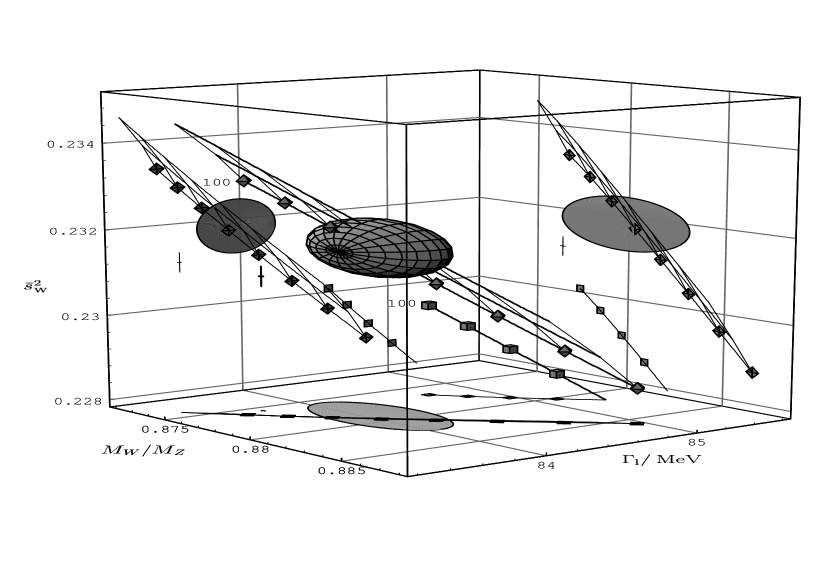
Figure 6: The need for $W$ loops from the present data (taken from [12]). See the text for full explanation and comment on this plot.

The “ball” is the $68\%$CL of the experimental data. The “net” that the ball hits is the full ${\cal{S}}{\cal{M}}\;$prediction and its array accounts for variations of $m_{t}$ and $M_{H}$. The $m_{t}$ line is depicted by diamonds starting with $m_{t}=100$ GeV and increasing by steps of 20 GeV towards the lower plane . This line corresponds to a fixed Higgs mass of 100 GeV. The other lines are for $M_{H}=300$ GeV and 1 TeV going from left to right. Keeping only the purely fermionic contribution gives the line with cubes again starting with $m_{t}=100$ GeV and increasing by steps of 20 GeV. It is clear that with $m_{t}\sim 180$ GeV the bosonic loops are mandatory. The thick cross represents the $\alpha(M_{Z}^{2})$-Born approximation that certainly also no longer works as an approximation, as it used to [13]. The projections into the corresponding two-dimensional plane which correspond to $83\%$CL are also shown. I think that the message is clear, it must be interpreted as an overwhelming support for the confirmation of the non-Abelian gauge structure of the ${\cal{S}}{\cal{M}}\;$. It is important to stress, as can be seen from the plots, that one can not infer much on the presence of the Higgs, let alone its mass. At the moment its contribution, that only enters as $\log(M_{H})$, can not be resolved experimentally. This dependence could also be interpreted as a cut-off dependence if the theory were formulated without the Higgs [2]. It is also amusing to note that there is an ambiguity with interpreting the data as prefering a scenario with or without a Higgs, since one should specify precisely how one subtracts the Higgs contribution, not to mention that setting a high value for the Higgs mass means that one has lost control on the perturbative expansion. In the analysis by Gambino and Sirlin [9], this contribution is subtracted à la $\overline{MS}$. The effect of the subtraction is equivalent to calculating within the ${\cal{S}}{\cal{M}}\;$with $M_{H}=113$ GeV. Thus, there is very little insight on the Higgs. This does not mean, on the other hand, that one has learnt absolutely nothing about symmetry breaking. It is now notoriously evident that some erstwhile popular (somehow natural) manifestations of technicolour do not stand the tests (see below).
This remark about the sensitivity of the present data on the Higgs is in order since whether the Higgs is light or heavy or absent has an incidence on the physics of $W$’s at the future colliders. Meanwhile, one should be extremely cautious when trying to interpret the results of some latest global fits (not just the leptonic and the $M_{W}/M_{Z}$ that were discussed previously) as indicating a preference for a light Higgs, the subtraction issue being only one aspect. As stressed by Langacker [14] in his latest global analysis of the precision data, “the preference for small $M_{H}$ is driven almost entirely by $R_{b}$ and $A_{LR}$ both of which differ significantly from the ${\cal{S}}{\cal{M}}\;$predictions. If these are due to large statistical fluctuations or to some new physics then the constraints on $M_{H}$ would essentially disappear.” As an illustration of this point, it is amusing to note that the discrepancy in $R_{b}$ has triggered an interest in technicolour rather than killed it. It has been argued that some unconventional (non-commuting) technicolour scenarios for symmetry breaking [15] may explain all existing data better than the ${\cal{S}}{\cal{M}}\;$.
As a conclusion about the impact of the low energy data on guiding us towards models of self-interacting $W$’s one should say that one should take the gauge invariance principle as sacrosanct but one should be open minded about the existence or the lightness of the Higgs.

4 The Hierarchy of couplings and their sizes

In view of the verification of the ${\cal{S}}{\cal{M}}\;$at better than the per-cent level (if one leaves aside the issue of $R_{b}$) and the confirmation of its inner workings at the quantum level, one should accept the fact that the model is a very good description of physics. Even though the fundamental issue of the Higgs is not resolved. One must also accept the principle of gauge invariance. But then how can one justify allowing the operators in Eq. 5 (that we argued describe residual effects of New Physics?) and which are obviously not gauge invariant under the full $SU(2)\times U(1)\,$local symmetry.

It is worth stressing again, contrary to the fierce attack [16] that blames the above HPZH Lagrangian (Eq. 5) for not being locally gauge invariant and leading to trouble at the quantum level, that as the lengthy introduction has shown all the above operators can be made gauge invariant, by unravelling and making explicit the compensating Goldstone fields and extra vertices that go with the above. As is evident with the mass terms, the term in Eq. 2 is not gauge invariant but this is only because it has been truncated from its larger part, Eq. 3 or Eq. 4. Under this light, the HPZH parametrisation should be considered as being written in a specific gauge and that after this gauge (unitary) has been chosen it is non-sensical to speak of gauge invariance [17, 1]. But of course, it is much much better to keep the full symmetry so that one can apply the Lagrangian to any situation and in any frame. There is another benefit in doing so. If the scale of new physics is far enough compared to the typical energy where the experiment is being carried out, then one should only include the first operators in the energy expansion, beyond those of the ${\cal{S}}{\cal{M}}\;$. Doing so will maintain some constraints on the parameters $\lambda,g_{1}^{Z},\Delta\kappa$. These constraints will of course be lost if you allow higher and higher order operators or allow strong breaking of custodial symmetry, in both cases rendering the situation chaotic while LEP1 shows and incredible regularity. It is highly improbable that the order and symmetry is perturbed so badly.

So what are these operators that describe the self-couplings when one restricts one-self to next-to-leading operators by exploiting the $SU(2)\times U(1)\,$and the custodial symmetry? and how are they mapped on the HPZH phenomenological parameters? The leading operators are of course those that describe the minimal standard model(Eqs. 3, 1 or it minimal Higgs-less version Eqs. 3, 1). These are given in Table 1 for the linear [18, 16] as well as the non-linear realisation [1, 19] to bring out some distinctive features about the two approaches:

Table 1: The Next-to-leading Operators describing the $W$ Self-Interactions which do not contribute to the $2$-point function.

Linear Realisation  ,   Light Higgs	Non Linear-Realisation  ,   No Higgs
${{\cal L}}_{B}=ig^{\prime}\frac{\epsilon_{B}}{\Lambda^{2}}({{\cal D}}_{\mu}\Phi)^{\dagger}B^{\mu\nu}{{\cal D}}_{\nu}\Phi$	${{\cal L}}_{9R}=-ig^{\prime}\frac{L_{9R}}{16\pi^{2}}{\rm Tr}({\mbox{\boldmath$B$}}^{\mu\nu}{{\cal D}}_{\mu}\Sigma^{\dagger}{{\cal D}}_{\nu}\Sigma)$
${{\cal L}}_{W}=ig\frac{\epsilon_{w}}{\Lambda^{2}}({{\cal D}}_{\mu}\Phi)^{\dagger}(2\times{\mbox{\boldmath$W$}}^{\mu\nu})({{\cal D}}_{\nu}\Phi)$	${{\cal L}}_{9L}=-ig\frac{L_{9L}}{16\pi^{2}}{\rm Tr}({\mbox{\boldmath$W$}}^{\mu\nu}{{\cal D}}_{\mu}\Sigma{{\cal D}}_{\nu}\Sigma^{\dagger})$
${{\cal L}}_{\lambda}=\frac{2i}{3}\frac{L_{\lambda}}{\Lambda^{2}}g^{3}{\rm Tr}({\mbox{\boldmath$W$}}_{\mu\nu}{\mbox{\boldmath$W$}}^{\nu\rho}{\mbox{\boldmath$W$}}^{\mu}_{\;\;\rho})$	$\;\;\;\;\;\;\;\;---------\;\;\;\;$
$\;\;\;\;\;\;\;\;---------\;\;\;\;$	${{\cal L}}_{1}=\frac{L_{1}}{16\pi^{2}}\left({\rm Tr}(D^{\mu}\Sigma^{\dagger}D_{\mu}\Sigma)\right)^{2}\equiv\frac{L_{1}}{16\pi^{2}}{{\cal O}}_{1}$
$\;\;\;\;\;\;\;\;---------\;\;\;\;$	${{\cal L}}_{2}=\frac{L_{2}}{16\pi^{2}}\left({\rm Tr}(D^{\mu}\Sigma^{\dagger}D_{\nu}\Sigma)\right)^{2}\equiv\frac{L_{2}}{16\pi^{2}}{{\cal O}}_{2}$

By going to the physical gauge, one recovers the phenomenological parameters with the constraints:

$$\Delta\kappa_{\gamma} = \frac{e^{2}}{s_{w}^{2}}\frac{v^{2}}{4\Lambda^{2}}(\epsilon_{W}+\epsilon_{B})=\frac{e^{2}}{s_{w}^{2}}\frac{1}{32\pi^{2}}\left(L_{9L}+L_{9R}\right)$$

$$\Delta\kappa_{Z} = \frac{e^{2}}{s_{w}^{2}}\frac{v^{2}}{4\Lambda^{2}}(\epsilon_{W}-\frac{s_{w}^{2}}{c_{w}^{2}}\epsilon_{B})=\frac{e^{2}}{s_{w}^{2}}\frac{1}{32\pi^{2}}\left(L_{9L}-\frac{s_{w}^{2}}{c_{w}^{2}}L_{9R}\right)$$

$$\Delta g_{1}^{Z} = \frac{e^{2}}{s_{w}^{2}}\frac{v^{2}}{4\Lambda^{2}}(\frac{\epsilon_{W}}{c_{w}^{2}})=\frac{e^{2}}{s_{w}^{2}}\frac{1}{32\pi^{2}}\left(\frac{L_{9L}}{c_{w}^{2}}\right)$$

$$\lambda_{\gamma} = \lambda_{Z}=\left(\frac{e^{2}}{s_{w}^{2}}\right)L_{\lambda}\frac{M_{W}^{2}}{\Lambda^{2}}$$ (7)

4.1 Quartic couplings

Note that $L_{9L,W,\lambda}$ do give quadri-linear bits but these are imposed by gauge invariance. This is confirmed by many analyses. Going to the physical gauge, the quartic couplings from the chiral approach are

$${{\cal L}}_{WWV_{1}V_{2}} = -e^{2}\left\{\left(A_{\mu}A^{\mu}W^{+}_{\nu}W^{-\nu}-A^{\mu}A^{\nu}W^{+}_{\mu}W^{-}_{\nu}\right)\right.$$ (8)

$$+ 2\frac{c_{w}}{s_{w}}(1+\frac{l_{9l}}{c_{w}^{2}})\left(A_{\mu}Z^{\mu}W^{+}_{\nu}W^{-\nu}-\frac{1}{2}A^{\mu}Z^{\nu}(W^{+}_{\mu}W^{-}_{\nu}+W^{+}_{\nu}W^{-}_{\mu})\right)$$

$$+ \frac{c_{w}^{2}}{s_{w}^{2}}(1+\frac{2l_{9l}}{c_{w}^{2}}-\frac{l_{-}}{c_{w}^{4}})\left(Z_{\mu}Z^{\mu}W^{+}_{\nu}W^{-\nu}-Z^{\mu}Z^{\nu}W^{+}_{\mu}W^{-}_{\nu}\right)$$

$$+ \frac{1}{2s_{w}^{2}}(1+2l_{9l}-l_{-})\left(W^{+\mu}W^{-}_{\mu}W^{+\nu}W^{-}_{\nu}-W^{+\mu}W^{+}_{\mu}W^{-\nu}W^{-}_{\nu}\right)$$

$$- \frac{l_{+}}{2s_{w}^{2}}\left(\left(3W^{+\mu}W^{-}_{\mu}W^{+\nu}W^{-}_{\nu}+W^{+\mu}W^{+}_{\mu}W^{-\nu}W^{-}_{\nu}\right)\right.$$

$$+ \frac{2}{c_{w}^{2}}\left.\left.\left(Z_{\mu}Z^{\mu}W^{+}_{\nu}W^{-\nu}+Z^{\mu}Z^{\nu}W^{+}_{\mu}W^{-}_{\nu}\right)+\frac{1}{c_{w}^{4}}Z_{\mu}Z^{\mu}Z_{\nu}Z^{\nu}\right)\right\}$$

$${\rm with}\;\;\;\;\;\;l_{9l}=\frac{e^{2}}{32\pi^{2}s_{w}^{2}}L_{9L}\;\;\;;\;\;\;l_{\pm}=\frac{e^{2}}{32\pi^{2}s_{w}^{2}}(L_{1}\pm L_{2})$$

Note that the genuine trilinear $L_{9L}$ gives structures analogous to the ${\cal{S}}{\cal{M}}\;$. The two photon couplings (at this order) are untouched by anomalies. The $L_{1,2}$, which have no equivalent at this order in the linear approach, contribute only to the quartic couplings of the massive states and thus genuinely describe quartic couplings.

4.2 Catch 22:

Aren’t there other operators with the same symmetries that appear at the same level in the hierarchy and would therefore be as likely?
Answer: YES. And this is an upsetting conceptual problem. On the basis of the above symmetries, one can not help it, but there are other operators which contribute to the tri-linear couplings and have a part which corresponds to bi-linear anomalous $W$ self-couplings. Because of the latter and of the unsurpassed precision of LEP1, these operators are already very much unambiguously constrained at the same level that operators describing a breaking of the global $SU(2)$ symmetry (especially after the slight breaking due to the $t-b$ mass shift has been taken into account). Examples of such annoying operators in the two approaches are

$${{\cal L}}_{WB} = gg^{\prime}\frac{\epsilon_{WB}}{\Lambda^{2}}\;\left(\Phi^{\dagger}\times{\mbox{\boldmath$W$}}^{\mu\nu}\Phi\right)B_{\mu\nu}$$

$${{\cal L}}_{10} = gg^{\prime}\frac{L_{10}}{16\pi^{2}}{\rm Tr}({\mbox{\boldmath$B$}}^{\mu\nu}\Sigma^{\dagger}{\mbox{\boldmath$W$}}^{\mu\nu}\Sigma)\longrightarrow L_{10}=-\pi S\simeq\frac{4\pi s_{W}}{\alpha}\epsilon_{3}$$ (9)

Limits on the coefficient $L_{10}$ from a global fit to the existing data are shown in the figure borrowed from [14], see Fig. 7. Allowance for a possible deviation of the $\rho$ parameter from unity (slight breaking of the global symmetry due to physics beyond the ${\cal{S}}{\cal{M}}\;$) is made: $\rho=1+\alpha T_{new}$.

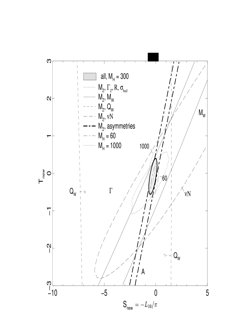
Figure 7: Present limits on $L_{10}$ and $T_{new}$. From [14]. The projection of the $L_{10}$ constraint from the fit is also shown (“bar”).

One can see that current limits indicate that $-0.7<L_{10}<2.4$ for a 2-parameter fit. This is really small, so small that if the other $L_{i}$’s, say, were of this order it would be extremely difficult to see an effect at the next colliders. So why should the still not-yet-tested operators be larger and/or provide more stringent tests? This is the naturalness argument which, in my view, is the essential point of [16]. One can try hard to find models with no contributions to $L_{10}$. One way out is to associate the smallness of $L_{10}$ to a symmetry that forbids its appearance, in the same way that the custodial $SU(2)$ symmetry prevents $\Delta\rho$ or leads to so small values of $T_{new}$. $L_{10}$ represents the breaking of the axial $SU(2)$ global symmetr [20]. But the construction of models is difficult. Models that make do with the $L_{10}$ constraint include some dynamical vector models that deviate from the usual scaled up versions of QCD by having (heavy) axial vectors like the extended BESS model [21]. The latter implements an $(SU(2)_{L}\times SU(2)_{R})^{3}$ symmetry, as discussed by D. Dominici in this volume. Axial vectors are included in the analysis presented in the talk of Tanabashi [22].

For the light Higgs scenario one has decoupling of the heavy particles so that the predicted $\epsilon_{WB}$ is small and does not have much incidence on the LEP1 data. A case in point is the minimal SUSY contribution. But at the same time one expects the other $\epsilon_{i}$ to be of the same order. The new physics in the light Higgs scenario may start to have an impact only if one is close to the threshold of production of the new particles which circulate in the loops. But then the effective approach through anomalous effective couplings is clearly not applicable. For instance, in $e^{+}e^{-}\rightarrow W^{+}W^{-}\;$one can not just subtract the parts that map into $\Delta g_{1}^{Z}$ etc… but one should take the full 1-loop contribution to the process, boxes for instance would not be negligible in these configurations. These expectations are borne out by explicit calculations [23]. One can, of course, hope to improve on the limits from LEP1, by exploiting the $k^{2}$ enhancement factor from these operators, in 2 fermion production as has been discussed by R. Szalapski in the parallel session [24].

To continue with my talk I will assume that $L_{10}\sim 0$ can be neglected compared to the other operators. This said, I will not completely ignore this limit and the message that LEP1 is giving us, $L_{10}\sim 1$, especially that various arguments about the “natural order of magnitude” [25] for these operators should force one to consider a limit extracted from future experiment to be meaningful if $|L_{i}|<\sim 10$. This translates into $\Delta\kappa,\Delta g^{1}_{Z}<\sim 10^{-2}$. Note that the present Tevatron limits if they were to be written in terms of $L_{9}$ give $L_{9}\sim 10^{3}$!!!

With this caveat about $L_{10}$ and the like, let us see how the 2 opposite assumptions about the lightness of the Higgs differ in their most probable effect on the $W$ self-couplings. First the tri-linear couplings $\lambda$ is relegated to higher orders in the heavy Higgs limit(less likely). This is as expected: transverse modes are not really an issue here. The main difference is that with a heavy Higgs, genuine quartic couplings contained in $L_{1,2}$ are as likely as the tri-linear and, in fact, when contributing to $WW$ scattering their effect will by far exceed that of the tri-linear. This is because $L_{1,2}$ involve essentially longitudinals. This is another way of arguing that either the Higgs exists or one should expect to “see something” in $WW$ scattering. Note also that $L_{9R,B}$ is not expected to contribute significantly in $pp\rightarrow WZ$ since it has no contribution to $\Delta g_{1}^{Z}$ (see Fig. 4). This is confirmed by many analyses.

5 Future Experimental Tests

With the order of magnitude on the $L_{i}$ that I have set as a meaningful benchmark, one should realise that to extract such (likely) small numbers one needs to know the ${\cal{S}}{\cal{M}}\;$cross sections with a precision of the order of $1\%$ or better. From a theoretical point of view this calls for the need to include the radiative corrections especially the initial state radiation. Moreover one should try to extract as much information from the $W$ and $Z$ samples: reconstruct the helicities, the angular distributions and correlations of the decay products. These criteria mean precision measurements and therefore we expect $e^{+}e^{-}\;$machines to have a clear advantage assuming that they have enough energy. Nonetheless, it is instructive to refer to Fig. 4 to see that $pp$ machines could be complementary.

In the following, one should keep in mind that all the extracted limits fall well within the unitarity limits. I only discuss the description in terms of “anomalous couplings” below an effective cms energy of a VV system $\sim 4\pi v\sim 3-4$ TeV, without the inclusions of resonances. Moreover, I will not discuss the situation when parameters are dressed with energy dependent form factors or any other scheme of unitarisation that introduces more model dependence on the extraction of the limits. These limits are given in terms of the chiral lagrangian parameters $L_{9L,R}$ or equivalently using Eq. 4 in terms of $L_{B,W}$. They can also be re-interpreted in terms of the more usual $\kappa_{V},g_{1}^{Z}$ with the constraint given by Eq. 4, in which case the $L_{9L}$ axis is directly proportional to $\Delta g^{1}_{Z}\;$. The reason for prefering to give the limits in the parameterisation $L_{9L}-L_{9R}$ is that, as argued above, by the time the NLC is built and run a few days one will know whether the Higgs is there or not, if it had not been discovered before. If it is around, the most interesting physics will be that of the Higgs and most likely supersymmetry. It is unlikely that one would learn more about symmetry breaking by searching for anomalous couplings in the tri-linear and quadri-linear couplings (that would have to be implemented through the linear approach) than by probing the supersymmetric spectrum or critically probing the properties of the Higgs [26].

5.1 Tri-linear couplings

In principle all $W/Z$ production processes could be used to search for possible anomalies in the self-couplings. As seen from Fig. 1 there are quite a few mechanisms. It is however clear that the best are those that have the largest cross sections and that are cleanest, especially after implementing the acceptance factors. Some of the largest cross sections are mostly due to forward events due to t-channel structures that are mostly dominated by transverse states, and consequently are less interesting. In this respect $e^{+}e^{-}\rightarrow W^{+}W^{-}\;$is one of the most promising and important cross sections. The full radiative corrections have been computed by two different groups and the results are found to agree perfectly [27]. These corrections are quite large and are due essentially to initial state radiation (ISR) in particular from the hard collinear photons. The latter drastically affect some of the distributions which, at tree-level, seem to be good New Physics discriminators because they are responsible for the boost effect that redistributes phase space: this leads to the migration of the forward $W$ (dominated by the t-channel neutrino contribution) into the backward region and results in a large correction in the backward region. Precisely the region where one would have hoped to see any s-channel effect more clearly. Second, if one reconstructs the polarisation of the $W$ without taking into account the energy loss, one may “mistag” a transverse $W$ for a longitudinal, thereby introducing a huge correction in the small tree-level longitudinal cross sections, which again is particularly sensitive to New Physics. Since at the NLC one has to take into account not only the bremsstrahlung but also the important beamstrahung contribution to the ISR, this contamination must be reduced to a minimum. Fortunately, there is a variety of cuts to achieve this, such as accolinearity cuts or keeping into the useful event samples only those events where the energies of the $W$’s add up to the cms energy. One welcome feature at the Linear Collider energies, compared to LEP2, is that $\cal O(\alpha^{2})$ corrections are negligible; moreover we do not have to worry about Coulomb singularities [28]. The latter enhance the cross section of a pair of slowly moving particles which have opposite charges. As for the genuine weak corrections the upshot is that the use of $G_{F}$ and a running $\alpha_{em}$ absorbs a large part of the weak corrections [29]. As a results there is no $m_{t}^{2}$ dependence, however some mild log dependence on the heavy particles (notably the Higgs) may survive. The latter could be responsible for delaying unitarity to higher energies and from this point of view mimick the effect of anomalous couplings.
In actual life the $W$’s are only observed through their decay products and therefore the $W$-pair production observables are in fact $4$-fermion observables. Unfortunately not all the 4-f observables are intimately related to the doubly resonant $WW$ production. Depending on the final state many other 4-f final states (especially with electrons) that do not proceed via $WW$ are present, see Fig. 8.

Figure 8: Four-fermion production classes of diagrams from [30].

The extra processes for $4$-f production could be potential background to $WW$ production and most importantly could mask the subtle effect that one would like to extract. Hence the need to know their cross sections as precisely as possible and find ways to subtract them. This subtraction, for instance requiring the invariant mass of both pairs of fermions to be consistent with the $W$ mass within the experimental resolution, can be done but at the expense of less statistics. Not that this is a problem with $WW$. From a theoretical point of view one can formally always find a prescription for isolating the $WW$ process. One may also prefer to keep all final states especially that there are topologies which are not associated with $WW$ production but which nevertheless involve the tri-linear couplings. Single-$W$ production as materialised through a fusion process (see Fig. 8) is such a process. It is then worth implementing non-standard couplings to the complete set of diagrams that lead to $4$-f and see if the sensitivity is enhanced. Many programs that calculate 4-fermion final states have been developped recently, especially for LEP2 [31, 32]. These should be optimised when moving to higher energies. Not all of them calculate all configurations of 4f. Those that involve electrons in the final states are hardest to calculate especially if one wants to keep the electrons exactly forward. In fact only a few manage to do this since this requires to keep the electron mass explicitely. Moreover one has to be careful with the implementation of the $W$ width. The problem of how to introduce the $W$ width is quite subtle and it is fair to say that at the moment though a few schemes have been suggested [33, 34, 35] there is no definite answer as yet on how to handle the width.
So at the moment one has full radiative corrections to the doubly resonant $WW$ process (as if the $W$ were stable) and full contributions to the $2\rightarrow 4$ process at tree-level only. The best of both worlds is to have the radiatively corrected $4$ final states. This is a horrendous task. However it is good to know that what one expects to be the largest corrections, ISR, can be easily implemented. Almost all of the $4$-fermion codes convolute with a radiator. Some codes like grc4f [36] can implement all ingredients: non-zero fermion masses, ISR, polarisation and anomalous couplings.

For extracting, or putting limits, on the anomalous couplings some extensive studies that aim at getting all the information which is contained in the 4f final states have been performed. As we stressed all along, the most important part is the longitudinal part of the $W$, which can be reconstructed by looking at the angular distributions of the fermion that results from the decay the $W$. In fact because of the $V-A$ structure of the $W$ interaction to fermions, these angular distributions (both polar $\theta_{i}$ and azimuthal $\phi_{i}$, the latter requires tagging the charge of the fermion) constitute an excellent polarimeter. Ideally one would like to have access to all the helicity amplitudes and the density matrix elements of the $WW$ process. Of course this neglects non resonant $WW$ diagrams or presumes the invariant mass cuts to be rather stringent such that one only ends up with the $WW$ process. Until very recently this has been the most widely used approach. In this approximation the theoretical issues are quite transparent. One starts from the helicity amplitudes of the $e^{+}e^{-}(\lambda)\rightarrow W^{-}(\tau_{1})W^{+}(\tau_{2})$ where $\lambda,\tau_{1,2}$ are the respective helicities. “Assuming” that one knows the velocity of the $W$ (or three momentum $|\vec{p}|$), which means that some “kneading” has been done about controlling ISR, and also the decay angles of the charged fermion as measured in the rest frame of the parent $W$ ($\theta_{i}$,$\phi_{i}$ $i=1,2$), all the information is contained in the five-fold differential cross section

$$\frac{{\rm d}\sigma(e^{+}e^{-}\rightarrow W^{+}W^{-}\;\rightarrow f_{1}\bar{f}_{2}f_{3}\bar{f}_{4})}{{\rm d}\cos\theta{\rm d}\cos\theta_{1}{\rm d}\phi_{1}{\rm d}\cos\theta_{2}{\rm d}\phi_{2}}=Br^{f_{1}\bar{f}_{2}}Br^{f_{3}\bar{f}_{4}}\frac{1}{16\pi s}\frac{|\vec{p}|}{\sqrt{s}}\left(\frac{3}{8\pi}\right)^{2}$$

$$\sum_{\lambda\tau_{1}\tau_{2}\tau^{\prime}_{1}\tau^{\prime}_{2}}F_{\tau_{1}\tau_{2}}^{\lambda}(s,\cos\theta)\;F_{\tau^{\prime}_{1}\tau^{\prime}_{2}}^{*\lambda}(s,\cos\theta)\;D_{\tau_{1}\tau^{\prime}_{1}}(\theta_{1},\phi_{1})\;D_{\tau_{2}\tau^{\prime}_{2}}(\pi-\theta_{2},\phi_{2}+\pi)$$

$$\equiv\frac{{\rm d}\sigma(e^{+}e^{-}\rightarrow W^{+}W^{-}\;)}{{\rm d}\cos\theta}\left(\frac{3}{8\pi}\right)^{2}\sum_{\tau_{1}\tau_{2}\tau^{\prime}_{1}\tau^{\prime}_{2}}\rho_{\tau_{1}\tau_{2}\tau^{\prime}_{1}\tau^{\prime}_{2}}\;D_{\tau_{1}\tau^{\prime}_{1}}(\theta_{1},\phi_{1})\;D_{\tau_{2}\tau^{\prime}_{2}}(\pi-\theta_{2},\phi_{2}+\pi)$$ (10)

$\theta$ is the scattering angle of the $W$ and $\rho$ is the density matrix that can be projected out. Note that one separates the decay and the production parts. To be able to reconstruct the direction of the charged $W$ and to have least ambiguity the best channel is the semi-leptonic channel $W^{\pm}\rightarrow l\nu_{l},W^{\mp}\rightarrow jj$ with $l=e,\mu$. Note however that if the charge of the jet is not reconstructed then we can not fully reconstruct the helicity of the $W$ that decays into jets, though an averaging may be done. It is also important to take into account initial electron polarisation, this in fact helps. For instance we can choose to concentrate on the $s$-channel only where the anomalous contribute, even if the statistics are lower. The BMT collaboration [37] has exploited the above approach where the fit has been done on the reconstructed density matrix elements and the limits on the parameters of the anomalous operators are extracted through a $\chi^{2}$ minimisation method. It is found [38] that the limits are much improved if one fits directly on the $5$ angular variables and uses a maximum likelihood method. Barklow [39] has also implemented this latter approach and looked also at the effect of ISR and beam polarisation at the linear collider. Preliminary investigations indicate that one can improve on the limits by also including the $4$-jets sample and perhaps the $\tau$ final state [40].
Alternatively, one would like to fit on all the available variables of the complete set of a particular $4$-f final state and not restrict the analysis to the resonant diagrams. Excalibur [41], Erato [42] and grc4f [36] allow to do such an analysis even with the inclusion of ISR. grc4f can even study single $W$ production (no cut on the forward electron), for a preliminary analysis see [43]. A thorough investigation for the linear collider energies taking into account the final $W$ width (all diagrams) using the maximum likelihood fit method has been done by Gintner, Godfrey and Couture [44]. ISR is not implemented but their results which we will comment upon in a moment, are quite telling especially that one can compare them with those based on the resonant diagrams.

5.2 Other Processes at and other modes of the linear collider

Perhaps the only disadvantage with the $WW$ process is that it is not easy to disentangle the $WW\gamma$ from the $WWZ$ couplings. To single out one of them one can exploit $e^{+}e^{-}\;\rightarrow\nu\nu_{e}\gamma$ [45] or $e^{+}e^{-}\;\rightarrow\nu\nu_{e}Z$ [46]. However, it should be pointed out that in specific models or in the chiral approach for example, the $WW\gamma$ and $WWZ$ couplings are related, see Eq. 4. Taking these constraints into account, the latter reactions do not seem to be competitive with $WW$. One of the reasons, especially for $\nu\nu\gamma$, is that the helicity structure is not as rich as in $WW$: all final particles do not have “interesting helicities”. $WW\gamma$ and $WWZ$ [47] production in $e^{+}e^{-}\;$are quite interesting but, as far as tri-linear couplings are concerned, they can compete with the $WW$ only for TeV energies since they suffer from much lower rates [47]. However they are very suited to study possible quartic couplings. In this respect $WWZ$ can probe the all important $L_{1,2}$.
In the $e^{-}e^{-}\;$mode one can investigate the tri-linear couplings through $e^{-}e^{-}\rightarrow e^{-}W^{-}\nu$ [48] this may be considered as the equivalent $e^{+}e^{-}\;$reaction $e^{+}e^{-}\;\rightarrow\nu\nu_{e}Z$ and has the same shortcomings. Cuypers has investigated the potential of this reaction in probing the tri-linear couplings by taking into account the possibility of polarised beams, fits have only been done to the scattering angle of the the final electron.
The $\gamma\gamma$ mode is of course ideal for the photonic couplings especially that here the cross section for $WW$ production is huge [49]. In the chiral approach this reaction will only constrain the combination $L_{9L}+L_{9R}$, but as we will see, in conjunction with the $e^{+}e^{-}\;$mode this is quite helpful. To probe the $WWZ$ couplings in $\gamma\gamma\;$one can use the rather large $WWZ$ [50, 51] rate. The corresponding reactions in the $e\gamma$ mode are  $e\gamma\rightarrow W\nu$ [52] and $e\gamma\rightarrow W\nu Z$ [53]. As with the two-body reaction in $e^{+}e^{-}\;$($e^{+}e^{-}\rightarrow W^{+}W^{-}\;$), the radiative corrections for $e\gamma\rightarrow W\nu$ [54] and $\gamma\gamma\rightarrow W^{+}W^{-}$ [55] have been calculated.

5.3 Limits from the LHC

Before discussing the limits on the parameters of the chiral Lagrangian that one hopes to achieve at the different modes of the linear colliders it is essential to compare with the situation at the LHC. For this we assume the high luminosity option with 100 fb^-1. These limits are based on a very careful study [56] that includes the very important effect of the QCD NLO corrections as well as implementing the full spin correlations for the most interesting channel $pp\rightarrow WZ$. $WW$ production with $W\rightarrow jets$ production is fraught with a huge QCD background, while the leptonic mode is extremely difficult to reconstruct due to the 2 missing neutrinos. Even so, a thorough investigation (including NLO QCD corrections) for this channel has been done [57], which confirms the superiority of the $WZ$ channel as we will see. The NLO corrections for $WZ$ production are huge, especially in precisely the regions where the anomalous are expected to show up, for instance, high $p_{T}^{Z}$. In the inclusive cross section this is mainly due to, first, the importance of the subprocess $q_{1}g\rightarrow Zq_{1}$ (large gluon density at the LHC) followed by the “splitting” of the quark $q_{1}$ into $W$. The probability for this splitting increases with the $p_{T}$ of the quark (or Z): Prob$(q_{1}\rightarrow q_{2}W)\sim\alpha_{w}/4\pi ln^{2}(p_{T}^{2}/M_{w}^{2})$. To reduce this effect one has to define an exclusive cross section that should be as close to the LO $WZ$ cross section as possible by cutting on the extra high $p_{T}$ quark (dismiss any jet with $p_{T}^{{\rm jet}}>50\ GeV,|\eta_{{\rm jet}}|<3$). This defines a NLO $WZ+``0{{\rm jet"}}$ cross section which is stable against variations in the choice of the $Q^{2}$ but which nonetheless can be off by as much as $20\%$ from the prediction of Born ${\cal{S}}{\cal{M}}\;$result.

6 Comparisons and Discussion

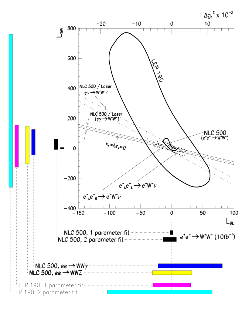
Figure 9: Comparison between the expected bounds on the two-parameter space $(L_{9L},L_{9R})\equiv(L_{W},L_{B})\equiv(\Delta g_{1}^{Z},\Delta\kappa_{\gamma})$ (see text for the conversions) at the NLC500 (with no initial polarisation) and LEP2. The NLC bounds are from $e^{+}e^{-}\rightarrow W^{+}W^{-}\;,W^{+}W^{-}\gamma,W^{+}W^{-}Z$ (for the latter these are one-parameter fits), $\gamma\gamma\rightarrow W^{+}W^{-}$ and $e^{-}e^{-}\rightarrow W^{-}\nu e^{-}$. Limits from a single parameter fit are also shown (“bars”).

The aim of the comparison is to show not only how well the different modes of the linear collider perform on bounding the parameters of the chiral Lagrangian but also how different fitting procedures constrain these couplings. In Fig. 9 we show the results of $\chi^{2}$ fits, assuming in the case of a 500 GeV a total luminosity of only 10 fb^-1. The bounds from $e^{+}e^{-}\;$are from the BMT [37] analysis adapted to the chiral approach. The limit from $e^{-}e^{-}\;$are from an analysis by Frank Cuypers. The $\gamma\gamma\;$analysis is adapted from [58].
First one sees that there is an incredible improvement on the bounds expected from LEP2 when going to 500 GeV. At this point a remark is in order. Complying with the benchmark values on the $L_{i}$ that one has set, the limits one expects to extract with a luminosity of $500$ pb^-1 at an energy of 190 GeV at LEP2 are not interesting from the point of view of symmetry breaking and precision. One only needs to contrast the situation with LEP1 and the equivalent plot of Fig. 7. These limits, though better than those from the Tevatron, are still not meaningful even if one restricts to one parameter fits. Moving from two parameters to one, we gain a factor of three at 190 GeV. But still in this case one has $|L_{9L}|<30$ and $-125<L_{9R}<155$. For such values the effective Lagrangian based on the chiral expansion is not meaningful and one should stick with the phenomenological parameterisation. As advertised the limits from $\gamma\gamma$ are quite competitive with those from $e^{+}e^{-}\;$at 500 GeV. The $e^{-}e^{-}\;$does not bring much information and does not usefully compete with the $e^{+}e^{-}\;$or even the $\gamma\gamma\;$options. Three vector production in $e^{+}e^{-}\;$, $WW\gamma$ and $WWZ$, are also not very helpful at 500 GeV from the point of view of checking the tri-linear couplings as indicated in the plot.

More recent analyses on the NLC have exploited the maximum likelihood technique and taken into account larger luminosities. First, the issue of the finite width can be quantified. Gintner, Godfrey and Couture [44] considered all diagrams that contribute to to the semi-leptonic $WW$ final state. By double mass constraint (10 GeV within $M_{W}$) one picks up essentially the double resonant process and compares this with the limits based on the same technique of fitting on all 5 kinematical variables. One sees, Fig. 10, that basing the analysis on the resonant diagrams very marginally degrades the limits. Therefore, after allowing for the $WW$ selection it seems that the limits based on the resonant diagrams can be totally trusted. To a very good approximation changing the luminosity can be accounted for by a scaling factor, $\sim\sqrt{{\cal L}}$, compare with the same analysis done with a reduced luminosity of 10 fb^-1. The latter should also be compared with the analysis reported in the previous plot and which is based on a $\chi^{2}$ fit. As discussed earlier the maximum likelihood fit does better. This is confirmed also by the analysis conducted by Tim Barklow [39] which assumes higher luminosities but take ISR into account as well as beam polarisation. For both the analyses at 500 GeV and 1.5 TeV the luminosity shown on the plot is shared equally between a left-handed and a right-handed electron (assuming $90\%$ longitudinal electron polarisation). With 80 fb^-1 (and almost similarly with 50 fb^-1) one really reaches the domain of precision measurements and one can truly contrast with the similar plot based on the LEP1 observables as concerns $L_{10}$ and $T_{new}$. It is quite fascinating that we can achieve this level of precision with such moderate energies. Moving to the TeV range one gains again as much as when moving from LEP190 GeV to 500 GeV, another order of magnitude improvement, see Fig. 10.

Figure 10: Limits on ($L_{9L}-L_{9R}$) in $e^{+}e^{-}\;$including ISR and beam polarisation with only the resonant diagrams. The effect of keeping all resonant diagrams for the semi-leptonic final state is also shown. Limits from $\gamma\gamma\rightarrow W^{+}W^{-}$ are also included. The LHC limits from $WZ$ and $W^{+}W^{-}$ are inserted also.

Returning to 500 GeV it is clear that the $\gamma\gamma$ option really helps. The results shown in Fig. 10 consider a luminosity of 20 fb^-1 with a peaked fixed spectrum corresponding to a cms $\gamma\gamma\;$energy of 400 GeV. This set up helps reduce the contour of the 80 fb^-1-500 GeV analysis in the $e^{+}e^{-}\;$mode. This very promising result is arrived at solely on the basis of the total cross section (with a moderate cut on the forward events). Only statistical errors were taken into account. We expect a much better improvement when a full spin analysis is conducted and fits using the maximum likelihood method are performed. During this Workshop the Hiroshima group [59] reported on a similar analysis with a full simulation. The electron energy was taken to be 250 GeV and the laser parameters were such that $x_{0}=4.7$. The original $e^{+}e^{-}\;$luminosity was assumed to be 40 fb^-1 and a realistic $\gamma\gamma\;$simulated. These $\gamma\gamma\;$results also confirm the power of the $\gamma\gamma\;$mode and lead to the bound $|L_{9L}+L_{9R}|<2.8$ at $90\%$CL.

Fig. 10 also compares the situation with the LHC. The limits on the parameters of the chiral Lagrangian have been adapted by Ulrich Baur from their detailed analysis that includes NLO QCD corrections, as outlined above when discussing the LHC. It is indeed found, as expected from the general arguments that I exposed above, refer to Fig. 4, that $L_{9L}$ is much better constrained than $L_{9R}$. As expected, the $WZ$ channel does a much better job since it does not suffer from the same ambiguity in the reconstruction of the final states and the background. Effectively $WZ$ (and hence $pp$) only constrains $L_{9L}$ through $\Delta g_{1}^{Z}$ that contributes a longitudinal $Z$. With 50 fb^-1 and 500 GeV the NLC constrains the two-parameter space much better than the LHC. The hadron collider is not very sensitive to $L_{9R}$. The sensitivity of the NLC is further enhanced if the experiments are done in conjunction with $\gamma\gamma\rightarrow W^{+}W^{-}\;$.

What about the genuine quartic couplings, as parameterised through $L_{1,2}$. These are extremely important as they involve essentially solely the longitudinal modes and hence are of crucial relevance when probing the Goldstone interaction. These are best probed through $V_{L}V_{L}\rightarrow V_{L}V_{L}$ scattering. However, with only 500 GeV the $V_{L}$ luminosity inside an electron is unfortunately not enough and one has to revert to $e^{+}e^{-}\;\rightarrow W^{+}W^{-}Z$ production, as suggested in [47]. This has been taken up by A. Miyamoto [60] who conducted a detailed simulation including $b$ tagging to reduce the very large background from top pair production. With a luminosity of 50 fb^-1 at 500 GeV, the limits are not very promising and do not pass the benchmark criterium $L_{i}<10$. It is found that $-95<L_{1}<71\;\;-103<L_{2}<100$ (one parameter fits). These limits agree very well with the results of a previous analysis [47]. To critically probe these special operators one needs energies in excess of 1 TeV, a preliminary study at 1 TeV indicates that the bounds can improve to $L_{1,2}\sim 6$. However, it is difficult to beat the LHC here, where limits of order $1$ are possible [61] through $pp\rightarrow W^{+}_{L}W^{+}_{L}$.

In conclusion, it is clear that already with a 500 GeV $e^{+}e^{-}\;$collider combined with a good integrated luminosity of about 50-80 fb^-1 one can reach a precision, on the parameters that probe ${\cal{S}}{\cal{B}}\;$in the genuine tri-linear $WWV$ couplings, of the same order as what we can be achieved with LEP1 on the two-point vertices. This would be an invaluable information on the mechanisms of symmetry breaking, if no particle has been observed at the LHC or …the NLC (Light Higgs and SUSY). The NLC is particularly unique in probing the vector models $L_{9}$ with $L_{1,2}\sim 0$ and hence is complementary to the LHC. The latter is extremely efficient at constraining the “scalar” models. To probe deeper into the structure of symmetry breaking, a linear collider with an energy range $\sqrt{s}>$ 1.5 TeV would be most welcome. In this regime there is also the fascinating aspect of $W$ interactions that I have not discussed and which is the appearance of strong resonances (refer too the talk of Tim Barklow). This would reveal another alternative to the ${\cal{S}}{\cal{M}}\;$description of the scalar sector.

Acknowledgements:
I am indebted to various friends and colleagues who have helped me with the talk by sending their results and answering many of my queries. I am particularly grateful to Ulrich Baur, Kingman Cheung, Frank Cuypers, Markus Gintner, Steve Godfrey, George Gounaris, Ken-ichi Hikasa, Jean-Loic Kneur, Yoshimasa Kurihara, Klaus Moenig, Akiya Miyamoto, Robert Sekulin, Rob Szalapski and Tohru Takahashi. I would also like to thank Marc Baillargeon and Geneviève Bélanger for the enjoyable collaboration. I am grateful to the organisers for the financial support of this excellently organised workshop. At last but not least, I would like to thank all the members of the Minami-Tateya group for a most enjoyable and memorable stay in Japan.

References

- [1] F. Boudjema, Proceedings of the Workshop on Physics and Experiments with Linear Colliders, eds. F.A. Harris et al.,, World Scientific, 1994, p. 712.
-
[2]
T. Appelquist, in “Gauge Theories and Experiments at High Energy”, ed.
by K.C. Brower and D.G. Sutherland, Scottish Univ. Summer School in Physics,
St. Andrews (1980).
See also, J.M. Cornwall, D.N. Levin and G. Tiktopoulos, Phys. Rev. D4 (1974) 1145. - [3] T. Barklow, these proceedings.
- [4] F. Boudjema and C. Hamzaoui, Phys. Rev. D43 (1991) 3748.
- [5] K. Hagiwara, R. Peccei, D. Zeppenfeld and K. Hikasa Nucl. Phys. B282 (1987) 253.
- [6] T. D. Lee, Phys. Rev. 140 (1965) 967.
-
[7]
F. Abe et al., CDF Coll., Phys. Rev. Lett. 74 (1995) 1936; ibid
75 (1995) 1017.
S.Abachi et al., D0 Coll., Phys. Rev. Lett. 75 (1995) 1034; ibid Submitted to HEP95 and Lepton-Photon 95, FERMILAB-Conf-95/250-E, hep-ex/9507014. - [8] Particle Data Group, Review of Particle Properties, Phys. Rev. D50 (1994) 1173.
- [9] P. Gambino and A. Sirlin, Phys. Rev. Lett. 73 (1994) 621.
- [10] S. Dittmaier, D. Schildknecht and M. Kuroda Nucl. Phys. B426 (1994).
- [11] A. Sirlin, Phys. Rev. D22 (1980) 971; W. J. Marciano and A. Sirlin, Phys. Rev. D22 (1980) 2695.
- [12] S. Dittmaier, D. Schildknecht and G. Weiglein, Nucl. Phys. B465 (1996) 3. hep-ph/9510386.
- [13] V.A. Novikov, L.B Okun, A.N. Rozanov and M.I. Vysotsky, Mod. Phys. Lett. A9 (1994) 2641.
- [14] P. Langacker, NSF-ITP-95-140, UPR-0683T, Oct. 1995.
- [15] E. H. Simmons, R. S. Chivukula and J. Terning, hep-ph/9511439.
- [16] A. de Rújula, M.B. Gavela, P. Hernandez and E. Massó, Nucl. Phys. B384 (1992) 3.
- [17] C.P. Burgess and D. London, Phys. Rev. Lett. 69 (1993) 3428; ibid Phys. Rev. D48 (1993) 4337.
- [18] W. Buchmüller and D. Wyler, Nucl. Phys. B268 (1986) 621.
- [19] B. Holdom, Phys. Lett. B258 (1991) 156.
- [20] T. Inami, C. S. Lim and A. Yamada, Mod. Phys. Lett. A7 (1992) 2789. See also, T. Inami, C. S. Lim in Proceedings of INS Workshop “Physics of , and Collisions at Linear Accelerators, edts Z. Hioki, T. Ishii and R. Najima, p.229, INS-J-181, May 1995.
- [21] R. Casalbuoni, S. De Curtis, D. Dominici and R. Gatto, Phys. Lett. B155, 95 (1985); Nucl. Phys. B282 (1987) 235. For extended BESS see, R. Casalbuoni et al., UGVA-DPT 1995/10-96, hep-ph/9510431.
- [22] K. Hikasa and Tanabashi, this volume.
-
[23]
See Masiero, in this volume.
A.B. Lahanas and V.C Spanos, Phys. Lett. B334 (1994) 378.
A. Arhrib, J. L. Kneur and G. Moultaka, as reported in the Report on Triple Gauge Boson Couplings, conveners G. Gounaris, J. L. Kneur, D. Zeppenfeld, LEP2 Yellow Book, CERN 96-01, Vol. 1, p. 525, edt. by G. Altarelli, T. Sjöstrand and F. Zwirner. - [24] See R. Szalapski, in this volume.
- [25] For a review see, J. Wudka Int. J. Mod. Phys. A9 (1994) 2301.
-
[26]
G. Gounaris and F. M. Renard, Phys. Lett. B236 (1994) 131; ibid Z. Phys. C59 (1993) 143.
K. Hagiwara and M.L Stong, Z. Phys. C62 (1994) 99.
G. Gounaris, F. M. Renard and N. D. Vlachos, Nucl. Phys. B459 (1996) 51. hep-ph/9509316. -
[27]
M. Böhm, A. Denner, T. Sack, W. Beenakker, F.A. Berends and H. Kuijf, Nucl. Phys. B304 (1988) 463.
W. Beenakker, K. Kołodziej and T. Sack, Phys. Lett. B258 (1991) 469;
W. Beenakker, F.A. Berends and T. Sack, Nucl. Phys. B367 (1991) 287.
K. Kołodziej and M. Zrałek, Phys. Rev. D43 (1991) 3619;
J. Fleischer, F. Jegerlehner and K. Kołodziej, Phys. Rev. D47 (1993) 830. -
[28]
V. S. Fadin, V. .A. Khoze and A.D. Martin, Phys. Lett. B311 (1993) 311.
D. Yu. Bardin, W. Beenakker and A. Denner, Phys. Lett. B317 (1993) 213.
V. S. Fadin al., Phys. Rev. D52 (1995) 1377. - [29] For a nice review on the radiative corrections too and related issues, see W. Beenakker and A. Denner, Int. J. Mod. Phys. A9 (1994) 4837.
- [30] T. Riemann, in this volume.
- [31] See the Standard Model Processes report, conv. F. Boudjema and B. Mele, in the LEP2 Yellow Book, CERN 96-01, p. 207, Vol. 1, edt. by G. Altarelli, T. Sjöstrand and F. Zwirner.
- [32] See the Event Generators for report, conv. D. Bardin and R. Kleiss, in the LEP2 Yellow Book, p. 3,Vol. 2, Op. cit.
- [33] Y. Kurihara, D. Perret-Gallix and Y. Shimizu, Phys. Lett. B349 (1995) 367; J. Fujimoto, T. Ishikawa, S. Kawabata, Y. Kurihara, Y. Shimizu and D. Perret-Gallix, Nucl. Phys. (Proc. Suppl.) 37B (1994) 169.
- [34] U. Baur and D. Zeppenfeld, Phys. Rev. Lett. 75 (1995) 1002.
- [35] E.N. Argyres et al., Phys.Lett. B358 (1995) 339.
- [36] T.Ishikawa, T.Kaneko, K.Kato, S.Kawabata, Y.Shimizu and K.Tanaka, KEK Report 92-19, 1993, The GRACE manual Ver. 1.0.
-
[37]
BMT: G.J. Gounaris et al., in Proc. of the Workshop on Collisions at 500 GeV: The Physics Potential, ed P. Zerwas, DESY-92-123B
(1992) 735.
BM2: M. Bilenky, J.L. Kneur, F.M. Renard and D. Schildknecht, Nucl. Phys. 409 (1993) 22. - [38] R.L. Sekulin, Phys. Lett. B338 (1994) 369.
- [39] T. Barklow, in the proceedings of the 8th DPF Meeting, Albuquerque, New Mexico, edt. S. Seidel, World Scientific p. 1236 (1995). (SLAC-PUB-6618).
- [40] J. B. Hansen, these proceedings. See also the report of the LEP2 Working Group Triple Gauge Boson Couplings G. Gounaris, J. L. Kneur and D. Zeppenfeld (conveners), LEP2 Yellow Book, in Press.
- [41] F.A.Berends, R.Pittau and R.Kleiss, Nucl. Phys. B424 (1994) 308; Comput. Phys. Commun. 85 (1995) 437. F. Berends and A. van Sighem, Nucl. Phys. B454 (1995) 467.
- [42] C. G. Papadopoulos, Phys. Lett. B333 (1994) 202; ibid B352 (1995) 144.
- [43] Y. Kurihara, Private Communication.
- [44] M. Gintner, S. Godfrey and G. Couture, Phys. Rev. D52 (1995).
-
[45]
G. Couture, S. Godfrey, Phys. Rev. D50 (1994) 5607.
K. J. Abraham, J. Kalinowski and P. Ściepko, Phys. Lett. B339 (1994) 136.
A. Miyamoto, in Proceedings of the Workshop on Physics and Experiments with Linear Colliders, p. 141, op. cit. - [46] S. Ambrosanio and B. Mele, Nucl. Phys. B374 (1992) 3; G. Couture, S. Godfrey and R. Lewis, Phys. Rev. D45 (1992) 777; G. Couture, S. Godfrey, Phys. Rev. D49 (1994) 5709.
- [47] G. Bélanger and F. Boudjema, Phys. Lett. B288 (1992) 201.
- [48] D. Choudhury and F. Cuypers, Phys. Lett. B325 (1994) 500.
- [49] For a list of references on this process, see G. Bélanger and F. Boudjema, Phys. Lett. B288 (1992) 210.
- [50] M. Baillargeon and F. Boudjema, Phys. Lett. B317 (1993) 371.
- [51] O. J. P. Eboli, M. B. Magro and P. G. Mercadante, Phys. Rev. D52 (1995) 3836. hep-ph/9508257.
-
[52]
I. F. Ginzburg,G. L. Lotkin, S. L. Panfil and V. G. Serbo, Nucl. Phys. B228
(1983) 285.
G. Couture, S. Godfrey and P. Kalyniak, Phys. Rev. D39 (1989) 3239.
E. Yehudai, Phys. Rev. D41 (1990) 44; ibid. (1991) 3434. S.Y. Choi and F. Schrempp, Phys. Lett. B272 (1991) 149.
K. J. Abraham and C. S. Kim, Phys. Lett. 301 (1993) 430.
M. Raidal, Nucl. Phys. B441 (1995) 49.
S. J. Brodsky, T. G. Rizzo and I. Schmidt, Phys. Rev. D52 (1995) 4929. hep-ph/9505441. - [53] K. Cheung, S. Dawson, T. Han and G. Valencia, Phys. Rev. D51 (1995) 5.
- [54] A. Denner and S. Dittmaier, Nucl. Phys. B398 (1993) 239 and 265.
-
[55]
A. Denner and S. Dittmaier and R. Schuster, Nucl. Phys. B452 (1995) 80.
G. Jikia, Talk given at Physics with Colliders, the European Working Groups, DESY, August 1995. - [56] U. Baur, T. Han and J. Ohnemus, Phys. Rev. D51 (1995) 3381. hep-ph/9410226.
- [57] U. Baur,T. Han and J. Ohnemus, Phys. Rev. D53 (1996) 1098. hep-ph/9507336.
- [58] M. Baillargeon, G. Bélanger and F. Boudjema, in Proceedings of Two-photon Physics from DANE to LEP200 and Beyond, Paris, eds. F. Kapusta and J. Parisi, World Scientific, 1995 p. 267; hep-ph/9405359.
- [59] T. Takahashi, these proceedings.
- [60] A. Miyamoto, these proceedings.
- [61] J. Bagger, S. Dawson and G. Valencia, Nucl. Phys. B399 (1993) 364.