Baryon Structure in a Covariant Diquark–Quark Model^∗

Abstract

The baryon structure is investigated in a covariant diquark-quark model. In this approach baryons emerge as relativistic bound states of a constituent quark and a $0^{+}$ or $1^{+}$ diquark. After solving the Bethe-Salpeter Equation for the scalar diquark quark system in ladder approximation we couple various external currents to the constituents of the baryon to probe its internal structure. The quark and the diquarks are assumed to be confined which is implemented by suitable choices for the propagators. This leads to nontrivial vertex functions between the constituents and the external current. Baryonic matrix elements are then evaluated to extract observable formfactors.

1 Introduction

The main goal of our work is to understand the baryon structure up to a momentum transfer of $Q^{2}\approx 1-2$ GeV. This momentum regime is particulary interesting because of the interplay between hadronic degrees of freedom on the one side and their intrinsic quark structure on the other side. To describe hadrons as bound states of quarks nonperturbative methods of QCD are unavoidable, whereas for large $Q^{2}$ the perturbative results of QCD should be met. So we are looking for an interpolating model to describe baryon structure at the intermediate energy region.

From the experimental side there is also an interest in this kind of calculations, because proposed and already started experiments (e.g. at COSY, ELSA, TJNAF) explore the baryon structure to a very high precision in this momentum regime.

This workshop is devoted to diquarks as a tool to parametrize complicated or unknown structures. We will exploit this philosophy in the following. Since a fully relativistic Faddeev equation which determines the nucleon as bound state of three quarks (bound by some kind of gluon interaction) is almost impossible to solve it is worthwhile to study the approximation where two quarks are bound to a diquark and interact with the third quark through quark exchange. Such a picture of a baryon has been derived by path integral techniques in the context of the Nambu–Jona-Lasinio model [1] and in the Global Color Model [2].
^∗ Supported by COSY under contract 41315266.

2 Bethe-Salpeter Equation for Baryons

The basic assumption of our model is that a baryon is a bound state of a constituent quark and a scalar ($0^{+}$) or axialvector ($1^{+}$) diquark which are bound due to quark exchange [1]. The corresponding Bethe-Salpeter equation (BSE) for the nucleon is then given by ,

$$\Phi(P,p)=\int\!\frac{d^{4}k}{(2\pi)^{4}}g(-k-p)\gamma_{5}S(-k-p)\gamma_{5}S(\textstyle{\frac{1}{2}}P+k)D(\textstyle{\frac{1}{2}}P-k)\Phi(P,k)$$

$$+\int\!\frac{d^{4}k}{(2\pi)^{4}}g(-k-p)\gamma^{\mu}S(-k-p)\gamma_{5}S(\textstyle{\frac{1}{2}}P+k)D^{\mu\nu}(\textstyle{\frac{1}{2}}P-k)\Phi^{\nu}(P,k)$$

$$\Phi^{\mu}(P,p)=\int\!\frac{d^{4}k}{(2\pi)^{4}}g(-k-p)\gamma_{5}S(-k-p)\gamma^{\mu}S(\textstyle{\frac{1}{2}}P+k)D(\textstyle{\frac{1}{2}}P-k)\Phi(P,k)$$

$$+\int\!\frac{d^{4}k}{(2\pi)^{4}}g(-k-p)\gamma^{\lambda}S(-k-p)\gamma^{\mu}S(\textstyle{\frac{1}{2}}P+k)D^{\lambda\rho}(\textstyle{\frac{1}{2}}P-k)\Phi^{\rho}(P,k)$$

(1)

where $\Phi(P,p)$ and $\Phi(P,p)^{\mu}$ are the baryon (scalar and axial vector) vertex functions with amputated quark and diquark legs. The quark propagator is denoted by $S(q)$ and the diquark propagator by $D(q)$ and $D^{\mu\nu}(q)$ respectively. $g(q)$ describes a possible extension of the diquark quark vertices. A solution of the Bethe-Salpeter equation which assumes a static quark exchange can be found in ref. [3]. Although $1^{+}$ diquarks are partially included in our calculation [4], we will restrict ourselves in the following to scalar diquarks so that only the first line of equation (1) survives.

Because $\Phi(P,p)$ describes a spin $\textstyle{\frac{1}{2}}$ particle it is useful to write it as a product of an amplitude $\Psi(P,p)$, which depends on the total and the relative momentum of the nucleon, and a Dirac spinor $u(P,S)$: [5]

$$\Phi(P,p):=\Psi(P,p)u(P,S).$$ (2)

After inserting this ansatz in the Bethe-Salpeter Equation (1), we multiply with the adjoint spinor $\bar{u}(P,S)$ from the right hand side and sum over the nucleon spins. It is the immidiately seen, that only the projections

$$\chi(P,p):=\Psi(P,p)\Lambda^{+},\qquad\Lambda^{+}=\frac{(-iP\!\cdot\!\gamma+M_{B})}{2M_{B}}$$ (3)

to positive energy survive. The projected amplitude $\chi(P,p)$ is then by construction an eigenfunction of $\Lambda^{+}$,

$$\chi(P,p)=\Psi(P,p)\Lambda^{+}=\chi(P,p)\Lambda^{+}.$$ (4)

This leads to the possibility to decompose further the Dirac structure of $\chi$ : The decomposition

$$\chi(P,p)=\textstyle{\frac{1}{2}}(1-i\frac{\gamma\!\cdot\!P}{M_{B}})S_{1}+\textstyle{\frac{1}{2}}(-i\gamma\!\cdot\!p_{T}-\frac{1}{2M_{B}}(\gamma\!\cdot\!p\gamma\!\cdot\!P-\gamma\!\cdot\!P\gamma\!\cdot\!p))S_{2},$$ (5)

is the only one compatible with equation (4). $p^{\mu}_{T}=p^{\mu}+P^{\mu}\frac{P\!\cdot\!p}{M^{2}_{B}}$ denotes the transversal relative momentum. The still unknown functions $S_{1}(P^{2},pP,p^{2})$ and $S_{2}(P^{2},pP,p^{2})$ are of course determined by the solution of the BSE.

In the rest frame of the bound state (where the actual calculations are done) we obtain

$$\chi_{\rm r.f.}(P,p)=\left(\begin{array}[]{cc}{\bf 1}S_{1}(P,p)&{\bf 0}\\ \mbox{\boldmath$\vec{\sigma}\vec{p}$}S_{2}(P,p)&{\bf 0}\end{array}\right).$$ (6)

It is now obvious that the first two columns of the $4\times 4$ matrix correspond to spinors with positive energy, spin up (“large” component) and spin down (“small” component) respectively. In the calculation of baryonic matrix elements we will restrict ourselves, in a first approximation, therefore to $S_{1}$.

Finally we expand the scalar functions $S_{j}(P,p),j=1,2$ in terms of Gegenbauer Polynomials [6]

$$S_{j}(P,p)=\sum_{k=0}^{\infty}i^{k}f_{k}^{j}(\sqrt{p^{2}})C_{k}^{1}(\frac{p\cdot P}{\sqrt{P^{2}}\sqrt{p^{2}}}),$$ (7)

and solve the Bethe-Salpeter Equation in the rest frame of the nucleon either by diagonalization or by iteration. In this way, the bound state mass is determined by the eigenvalue of the integral equation, while the expansion coefficients $f_{k}^{j}$ correspond to the eigenvectors.

2.1 Parametrization of confined constituents

Since neither quarks nor diquarks have ever been observed as asymptotic states in experiments, there is not much justification necessary to include this feature of QCD in a calculation of baryon properties.

We implement confinement by using propagators which have no poles. In case of the quark propagator this has to be understood as an effective parametrization of the behavior obtained in Dyson-Schwinger studies of QCD [7]. The quark self-energies which appear in

$$S(p)=-i\gamma\!\cdot\!p\sigma_{v}(p)+\sigma_{s}(p)=[i\gamma\!\cdot\!pA(p)+B(P)]^{-1}$$ (8)

are then choosen as

$$\sigma_{v}(p)=\frac{1-\exp(-(1+\frac{p^{2}}{m_{q}^{2}})}{p^{2}+m_{q}^{2}}\quad{\rm and}\quad\sigma_{s}(p)=m_{q}\sigma_{v}(p).$$ (9)

Obviously the exponentials remove the mass poles however, thereby introducing an essential singularity at $p^{2}=-\infty$.
In ref.[8] it has been shown that confined diquarks can be obtained when one uses an appropriate irreducible quark-quark kernel (beyond ladder approximation). We simulate this by using

$$D(p)=\frac{-iZ(p)}{p^{2}+m_{d}^{2}}$$ (10)

where

$$Z(p)=1-\exp(-(1+\frac{p^{2}}{m_{d}^{2}})).$$ (11)

Note that an elementary scalar diquark would correspond to $Z\equiv 1$. With such a prescription of confined constituents we especially get rid of the unphysical quark-diquark thresholds which plague baryon calculations within the pure hadronized NJL-model [9].
To estimate the effects of an intrinsic diquark structure we did the calculation with a pointlike quark-diquark coupling

$$g(k)=g_{0}$$ (12)

as well as with a diquark formfactor (see also ref. [10])

$$g(k)=g_{0}\frac{\Lambda^{2}}{k^{2}+\Lambda^{2}},$$ (13)

where $\Lambda$ is of the order of $2m_{q}$ and which simulates the diquark structure in a crude way.

Figure 1: Numerical Solution of the Bethe-Salpeter equation.The results in the left figure are obtained with a diquark formfactor, in the right figure with a pointlike coupling.

2.2 Numerical results

In Fig.1 the numerical results for the dominant expansion functions $f_{k}^{j}$ without and with a diquark formfactor are shown. The parameters here and in the following are fixed to $m_{q}=m_{d}=0.5$ GeV and the coupling is chosen to obtain $M_{B}=0.95$ GeV. In both figures the functions fall off rapidly for large relative momenta, but the asymptotic behavior is quite different: Assuming a diquark structure leads to a narrower amplitude in momentum space. This will also have an effect for the observables, where a possible diquark structure just enters via the nucleon vertex function. We observe that in both cases the expansion in terms of Gegenbauer Polynomials converge rather rapidly.

3 Hadronic matrix elements

3.1 Mandelstam’s formalism

Matrix elements of operators in the Bethe-Salpeter approach are calculated according to Mandelstam’s formalism [11]

$$\langle\hat{O}\rangle=\int\!\frac{d^{4}p}{(2\pi)^{4}}\int\!\frac{d^{4}p^{\prime}}{(2\pi)^{4}}{\bar{\psi}}(P^{\prime},p^{\prime})\Gamma_{\hat{O}}(p^{\prime},P^{\prime};p,P){\psi}(P,p).$$ (14)

Note that $P$ and $p$ ($P^{\prime}$ and $p^{\prime}$) are the total and relative momenta of the diquark-quark states before and after the interaction; ${\psi}$ is the normalized diquark-quark Bethe-Salpeter wave function related to the vertexfunction by multiplying with the quark and diquark propagator. The 5-point function $\Gamma_{\hat{O}}$ describes how the external current couples to all internal lines of the diquark-quark system.

In the following we work in a generalized impulse approximation, where we consider only the coupling to the quark and to the diquark,

$$\Gamma_{\hat{O}}(p^{\prime},P^{\prime};p,P)=\Gamma^{q}_{\hat{O}}(p^{\prime},P^{\prime};p,P)+\Gamma^{d}_{\hat{O}}(p^{\prime},P^{\prime};p,P),$$ (15)

and neglect the coupling to the exchanged quark.

3.2 Vertexfunctions of the constituents

In case of electromagnetic (e.m.) formfactors, we still have to know the quark-photon and the diquark-photon vertexfunctions. Using gauge symmetry, which is manifest in the Ward-Takahashi identity,

$$q_{\mu}i\Gamma_{\mu}(p,q,p+q)=S^{-1}(p+q)-S^{-1}(p)$$ (16)

one observes the connection of the longitudinal part of the vertexfunction and the inverse propagator.
A vertexfunction which solves the above identity for the quark is the Ball-Chiu vertex [12]

$$\Gamma_{\mu}^{BC}(p,k)=\frac{A(p^{2})+A(k^{2})}{2}\gamma_{\mu}+\frac{(p+k)_{\mu}}{p^{2}-k^{2}}\{(A(p^{2})-A(k^{2}))\frac{\gamma p+\gamma k}{2}$$

$$-i(B(p^{2})-B(k^{2}))\},$$ (17)

and in case of the diquark

$$\Gamma_{\mu}^{d}(p,k)=(p+k)_{\mu}\frac{D^{-1}(p)-D^{-1}(k)}{p^{2}-k^{2}}.$$ (18)

These vertexfunctions are totally determined by the self-energy functions of the corresponding propagators.

4 Electromagnetic nucleon formfactors

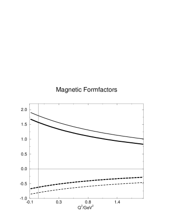
Figure 2: Electromagnetic Formfactors of the nucleon: The solid lines are the proton formfactors, the dotted lines the neutron formfactors; the thin curves are the results with a diquark formfactor, whereas the thick curves are the results assuming a pointlike quark-diquark coupling.

Within our approximations we decompose the matrix element into a quark and a diquark part

$$J_{\mu}(Q^{2})=Q_{q}J_{\mu}^{q}(Q^{2})+Q_{d}J_{\mu}^{d}(Q^{2}),$$ (19)

with the charge matrices in isospin space

$$Q_{q}=\textstyle{\frac{1}{2}}({\textstyle{\frac{1}{3}}}{\bf 1}_{\rm F}+\mbox{\boldmath$\tau$}_{z}),\quad Q_{d}={\textstyle{\frac{1}{3}}}{\bf 1}_{\rm F}.$$ (20)

The quark part is given by

$$J_{\mu}^{q}(Q^{2})=\int\!\frac{d^{4}k}{(2\pi)^{4}}\bar{\chi}(P_{f},p_{f})S_{q}(k_{+})i\Gamma_{\mu}^{BC}(k_{+},k_{-})S_{q}(k_{-})S_{d}(k_{d})\chi(P_{i},p_{i}),$$ (21)

whereas the diquark part is calculated with the loop diagram

$$J_{\mu}^{d}(Q^{2})=\int\!\frac{d^{4}k}{(2\pi)^{4}}\bar{\chi}(P_{f},p_{f})S_{d}(k_{+})i\Gamma_{\mu}^{d}(k_{+},k_{-})S_{d}(k_{-})S_{q}(k_{q})\chi(P_{i},p_{i}).$$ (22)

From Lorentz invariance and discrete symmetries it is also known that the onshell e.m. nucleon current can be decomposed into

$$J_{\mu}(Q^{2}) = \langle N(P_{f},S_{f})|j_{\mu}|N(P_{i},S_{i})\rangle$$

$$= \bar{u}(P_{f},S_{f})[iM_{B}(F_{e}(Q^{2})-F_{m}(Q^{2}))\frac{P_{\mu}}{P^{2}}+F_{m}(Q^{2})\gamma_{\mu}]u(P_{i},S_{i}).$$

Note that in our formalism the Dirac spinors appearing on the right hand side are replaced by the $\Lambda^{+}$ projectors. The Lorentz invariant functions $F_{e}(Q^{2})$ and $F_{m}(Q^{2})$ denote the electric and magnetic formfactor, respectively, which depend on the photon momentum $Q^{2}$. When the left hand side of this equation is calculated with the above loop diagrams in the Breit frame, $F_{e}(Q^{2})$ and $F_{m}(Q^{2})$ can be extracted by taking appropriate traces.

In Fig.2 the numerical results for the e.m. formfactors are shown. We observe that an internal diquark structure (leading to a narrower vertex function in momentum space) seems to be necessary in our approach because otherwise the variation of the formfactors with $Q^{2}$ around $0$ is only weak, the e.m. radii are then far too smalll. While the violation of charge conservation due to the impulse approximation can be compensated by choosing a suitable momentum distribution in the loop integrals, the absolute values of the magnetic moments are not large enough which means that $1^{+}$ diquarks are needed for a phenomenologically satisfying description. Since our model is covariant, timelike formfactors are also accessible, which can be seen in the figure: The formfactors are continous at $Q^{2}=0$.

5 Pion-nucleon formfactor

When following Mandelstam’s prescripton it is also possible to couple an external pion current to the nucleon. Because of parity there is no coupling to the (scalar) diquark, so there is just one diagram to calculate (in analogy to equation (21) but where the quark-photon vertex is replaced by the quark-pion vertex). The quark-pion vertex ( = pion Bethe-Salpeter amplitude) in the chiral limit ($m_{\pi}=0$) is determined by the scalar quark selfenergy

$$\Gamma_{5}^{a}(P^{2}=0,p^{2})=\gamma_{5}\frac{B(p^{2})}{f_{\pi}}\tau^{a},$$ (24)

as a consequence of chiral symmetry [13]. Furthermore the invariant parametrization of the pion-nucleon matrix element is given by

$$J_{5}^{a}(Q^{2}) = \langle N(P_{f},S_{f})|j_{5}|N(P_{i},S_{i})\rangle$$ (25)

$$= \bar{u}(P_{f},S_{f})[\gamma_{5}g_{\pi NN}(Q^{2})\tau^{a}]u(P_{i},S_{i}).$$

In analogy to the electromagnetic formfactors, $g_{\pi NN}$ on the right hand side of this equation can be extracted when the left hand side is evaluated with the diagram where the pion couples to the quark and the diquark remains a spectator.

Figure 3: Numerical Solutions for the Pion-Nucleon coupling $g_{\pi NN}(Q^{2})$. The thin curve denotes our results with the diquark formfactor, the thick curve our results without a formfactor.

Our numerical results for $g_{\pi NN}$ are displayed in Fig. 3. Again a diquark structure is unavoidable to get the expected variation of the formfactor with the pion momentum. The absolute value of $g_{\pi NN}$ at the pion mass shell ($Q^{2}=0$ in the chiral limit) is in remarkable agreement with the experimental value of about $14$.

6 Conclusion

In this talk we have presented a covariant bound state approach for the nucleon where quarks and diquarks interact through quark exchange. Using an effective parametrization of confinement we calculated within the needed approximations not only the nucleon mass and wave function but also electromagnetic and strong formfactors. It has been discussed that an internal diquark structure, entering through a diquark formfactor in the BSE is preferable to obtain a nucleon wave function which has a realistic width in momentum space. Furthermore the implementation of axialvector diquarks is necessary to improve the magnetic observables.

This work is just the first step towards a full satisfying baryon model of the proposed diquark-quark bound state approach. Nevertheless the results obtained so far are quite encouraging. To benefit from the advantages of our covariant and confining approach we will also apply this model to electromagnetic and strong $NN^{*}$ transitions, virtual Compton scattering and $\Lambda$-production.

References

References

- [1] H. Reinhardt, Phys. Lett. B 244 (1990) 316.
- [2] R. T. Cahill, Aust. J. Phys. 42 (1989) 171.
- [3] A. Buck, R. Alkofer, H. Reinhardt, Phys. Lett. B 286 (1992) 29.
- [4] In preparation.
- [5] H. Meyer, Phys. Lett. B337 (1994) 37.
- [6] T. Nieuwenhuis, J. A. Tjon, to appear in Few Body Systems 21 (1996).
- [7] C. D. Roberts, A. G. Williams, Prog. Part. Nuc. Phys. 33 (1994).
- [8] A. Bender, C. D. Roberts, L. v. Smekal, Phys. Lett. B 380 (1996) 7.
- [9] G. Hellstern, C. Weiß, Phys. Lett. B 351 (1995) 64.
- [10] K. Kusaka, G. Piller, A. W. Thomas, A. G. Williams, hep-ph/9609277.
- [11] S. Mandelstam, Proc. Roy. Soc. 233 (1955) 248.
- [12] J. S. Ball, T.W. Chiu, Phys. Rev. D 22 (1980) 2542.
- [13] R. Delbourgo, M. D. Scadron, J. Phys. G 5 (1979) 1621.