Abstract

The near–threshold expansion of the $\pi\pi$ amplitude is developed using the crossing–covariant independent variables. The independent threshold parameters entering the real part of the amplitude in an explicitly Lorentz–invariant way are free from restrictions of isotopic and crossing symmetries. Parameters of the expansion of the imaginary part are recovered by the perturbative unitarity relations.

Sankt–Petersburg 1996

Cross-Symmetric Expansion of $\pi\pi$ Amplitude Near Threshold

A.A. Bolokhov, T.A. Bolokhov, I.S. Manida

Sankt-Petersburg State University, Sankt-Petersburg, 198904, Russia

M.V. Polyakov, S.G. Sherman

St. Petersburg Institute for Nuclear Physics, Sankt–Petersburg, 188350, Russia

Abstract

The near–threshold expansion of the $\pi\pi$ amplitude is developed using the crossing–covariant independent variables. The independent threshold parameters entering the real part of the amplitude in an explicitly Lorentz–invariant way are free from restrictions of isotopic and crossing symmetries. Parameters of the expansion of the imaginary part are recovered by the perturbative unitarity relations.

1 Introduction

The growth of interest to the pion interactions is currently motivated by the achievements of the Chiral Perturbation Theory (ChPT) which was formulated by Weinberg, Gasser and Leutwyler [1, 2] as an effective low energy limit of QCD. Already first successful one–loop calculations of the near–threshold $\pi\pi$ amplitude by M. Volkov and Pervushin [3] had shown the predictive power of Chiral Symmetry in the framework of approach of nonlinear effective lagrangians (see [4]). The importance of the threshold characteristics of the $\pi\pi$ scattering explains also the need in more precise experimental measurements and the model–independent analysis of these characteristics.

During all the times being, the central role of the $\pi\pi$ scattering in the theory of strong interactions is steming from its remarkable properties which might be briefly collected into the following list:

1. Pions are the lightest hadronic states; unitarity provides that only the elastic $\pi\pi$ cut is important at low energies.

2. Pions are spinless particles: the amplitude assumes the simplest form.

3. The isospin symmetry restricts the amplitudes of various physical processes to only 3 independent combinations since the two–pion state might have only three values of the fixed isospin $I=2,\;1,\;0$.

4. This reaction provides an example of the perfect crossing symmetry. The three isospin amplitudes are still not independent in the functional sense. Bose–statistics of pions considered as identical particles and crossing relations for amplitudes of cross channels allow to express any two amplitudes in terms of the rest one.

5. The interpretation of the pion as the Goldstone boson of the spontaneously broken Chiral symmetry of QCD provided a new argumentation for the importance of the pion–pion interactions in the hadron physics and nuclear phenomena at low energies.

The few listed properties explain why this reaction for a long time serves as a test field for various methods of the quantum field theory such as dispersion relations, the $S$–matrix approach, etc. The advantages and achievements of various theoretical approaches are summarized in the review books [5, 6] — we advise reader to look there for more details if necessary; the modern point of view on pion–pion and pion–hadron interactions might be found in the book [7] and details of ChPT approach — in the review papers [8, 9]; a summary of the most interesting theoretical predictions as well as of the forthcoming experimental tests might be found in the talk [10].

The recent results [11] of the so called Generalized ChPT approach [12] and the progress in the two–loop ChPT calculations [13, 11] are claiming for more precise experimental information on the $\pi\pi$ interaction at low energies at the $O(k^{6})$ order which obviously must be presented in the model–independent form.

Since it is not possible experimentally to create the pionic target or the colliding pion beams there are only indirect ways for obtaining experimental data on the $\pi\pi$ scattering. The reactions $\pi N\to\pi\pi N$ and $K\to\pi\pi e{\nu}$ are considered as the most important sources of an (indirect) information. At the same time more extended variety of processes like $\gamma N\to\pi\pi N$ must rely upon the same properties of OPE mechanism and/or the final–state interaction of pions which are common to the description of $\pi N\to\pi\pi N$ and $K\to\pi\pi e{\nu}$ reactions. Therefore an unambiguous parametrization of the $\pi\pi$ amplitude ($4\pi$ vertex) is required for the low energy region.

In principle, the parameters of phase shifts or the scattering lengths and the slopes of partial waves are the most acceptable physical parameters. However, the partial wave decomposition can not respect the crossing properties in a simple way. The technique of Roy equations [14] based on dispersion relations can restrict the parameters and make the amplitude (which is defined in terms of partial waves) consistent with conditions of Bose–statistics and crossing. The approach relies upon high energy $\pi\pi$ data. Since the latter are neither infinitely precise nor free from contradictions only the bands for the scattering lengths had been provided in the most recent application of this approach in the paper [15].

The need to provide the analysis of data on processes like $\pi N\to\pi\pi N$, $\gamma N\to\pi\pi N$ where the amplitude of $\pi\pi$ scattering must be considered in the presence of contributions of a variety of concurrent processes puts further restrictions on the desired parametrization of the $4\pi$ vertex. Since the analyzed amplitude comes with a large number of free parameters the fitting of experimental data becomes possible only under the condition that the phase–space integration might be factored out from parameters. This is possible only if free (and formal) parameters enter the amplitude polynomially and the relations for formal parameters do not contain kinematics; otherwise the huge number of the 9–dimensional integration runs would be inevitable for all experimental points during the every step of fitting iterations.

The condition rules out the phase shift parameters as well as the next–to–leading order ansatz of ChPT for the $4\pi$ vertex.

The main goal of the present paper is to elaborate the near–threshold expansion of the $\pi\pi$ amplitude which along with the isospin invariance satisfies the exact combined Bose and crossing symmetries and the approximate (perturbative) unitarity.

Our approach is based on the crossing covariant variables which were introduced in the paper [16] and proved to be an efficient tool for the off–mass–shell parametrization of the considered amplitude, in particular, when being applied to the $\pi N\to\pi\pi N$ reaction [17]. In the present paper we use combinations of parameters describing the deviation from the threshold in the crossing–invariant way. In their terms the real part of the amplitude is uniformly expanded in the vicinities of the thresholds of all physical channels simultaneously. The region of validity of the expansion is in general restricted by the Mandelstam domain of analiticity [18]

$$|stu|<288\mu^{6}\;.$$ (1)

The paper is organized as follows. The content of the sect. 2 reminds definitions and basic properties of the considered amplitude. In sect. 3 the analysis of crossing properties of the amplitude is provided on the base of crossing covariant variables of the paper [16]. The results are used for the final construction of the low energy phenomenological amplitude in sect. 4. The summary, the concluding remarks and the discussion on the field of possible applications are given in Conclusions.

2 General Properties of $\pi\pi$ Amplitude

We shall consider the amplitude $M_{adbc}$ of the auxiliary reaction

$$\pi_{a}(k_{1})+\pi_{d}(k_{4})\rightarrow\pi_{b}(k_{2})+\pi_{c}(k_{3})\;,$$ (2)

and define it by

$$\langle\pi_{b}(k_{2}),\pi_{c}(k_{3})\;|\;S-1\;|\;\pi_{a}(k_{1}),\pi_{d}(k_{4})\rangle=i(2\pi)^{4}\delta^{4}(k_{1}+k_{4}-k_{2}-k_{3})M_{adbc}\;.$$ (3)

The amplitude of any physical process is obtained in terms of $M_{adbc}$ using the definitions of (charged) pion fields:

$$\pi^{\pm}=\frac{1}{\sqrt{2}}(\pi_{1}\pm i\pi_{2})\;,\;\pi^{0}=\pi_{3}\;.$$ (4)

The essence of the isotopic symmetry might be exploited in two ways. First, it allows to write $M_{adbc}$ in terms of the isospin projections (the direct $s$ channel is selected here):

$$M_{adbc}=P^{I=2}_{ad,bc}T^{2}+P^{I=1}_{ad,bc}T^{1}+P^{I=0}_{ad,bc}T^{0}\;,$$ (5)

$$P^{I=2}_{ad,bc}=-\frac{1}{3}\delta_{ad}\delta_{bc}+\frac{1}{2}(\delta_{bd}\delta_{ac}+\delta_{cd}\delta_{ab})\;;\;\;P^{I=1}_{ad,bc}=-\frac{1}{2}(\delta_{bd}\delta_{ac}-\delta_{cd}\delta_{ab})\;;\;\;P^{I=0}_{ad,bc}=\frac{1}{3}\delta_{ad}\delta_{bc}\;.$$ (6)

Second, one can define the isoscalar amplitudes $A,B,C$:

$$M_{adbc}=A\delta_{ad}\delta_{bc}+B\delta_{bd}\delta_{ac}+C\delta_{cd}\delta_{ab}\;,$$ (7)

related to the fixed–isospin amplitudes (5) by

$$T^{0}=3A+B+C\;;\;\;T^{1}=-B+C\;;\;\;T^{2}=B+C\;.$$ (8)

The kinematical variables are the usual Mandelstam ones

$$s=(k_{1}+k_{4})^{2}=(k_{2}+k_{3})^{2}\;;\;\;t=(k_{1}-k_{2})^{2}=(k_{4}-k_{3})^{2}\;;\;\;u=(k_{1}-k_{3})^{2}=(k_{4}-k_{2})^{2}\;,$$ (9)

which are restricted on the mass shell of the $4\pi$ vertex by

$$s+t+u=\sum_{i}\mu^{2}_{i}=4\mu^{2}\;.$$ (10)

To study the crossing properties it is suitable to consider $A,B,C$ as functions of all set $s,t,u$ ($A=A(s,t,u)$, etc.). Then the crossing properties of the amplitude combined with Bose–statistics of pions provide the conditions

$$A(s,t,u)=A(s,u,t)\;;\;B(s,t,u)=B(t,s,u)\;;\;C(s,t,u)=C(u,t,s)\;,$$ (11)

and the relations

$$B(s,t,u)=A(u,s,t)=C(t,u,s)\;.$$

These very properties look much more involved when formulated in terms of the decomposition (5). The latter is suitable for defining physical (observable) characteristics. It makes the strong preference of the $s$ channel, so the variables usually chosen as independent are $s$ and $t-u$ or the momentum in the Center of Mass Frame (CMF) $|{\bf k}|$ and the scattering angle ${\Theta}$:

$$s=4({\bf k}^{2}+\mu^{2})\;,\;t-u=4{\bf k}^{2}\cos\Theta\;.$$ (12)

Because of the residual symmetry in the decomposition (5) the amplitudes $T^{0}$ and $T^{2}$ must be symmetric with respect to the $(t\leftrightarrow u)$ permutation and, hence, have only even powers of the $(t-u)$ variable, while $T^{1}$ has only odd ones.

At the energies below the $4\pi$ threshold only the elastic unitarity conditions are of importance. They are obtained by inserting the 2–pion intermediate state into the unitarity condition for the $S$–matrix $S=1+iT$:

$$\frac{1}{i}(T-T^{{\dagger}})=TT^{{\dagger}}\;.$$ (13)

Because of the isospin conservation the resulting equations are diagonal in $T^{I}$. They assume simple algebraic form for the partial waves $T^{I}_{L}$ defined via

$$T^{I}=(32\pi)\sum_{L}(2L+1)P_{L}(\cos\Theta)T^{I}_{L}(|{\bf k}|)\;,$$ (14)

or

$$T^{I}_{L}=\frac{1}{(32\pi)}\frac{1}{2}\int^{1}_{-1}d\cos(\Theta)P_{L}(\cos\Theta)T^{I}\;.$$ (15)

The elastic unitarity requires

$${\rm Im}~{}T^{I}_{L}=\sigma(s)[({\rm Re}~{}T^{I}_{L})^{2}+({\rm Im}~{}T^{I}_{L})^{2}]\;.$$ (16)

where

$$\sigma(s)=\sqrt{\frac{s-4\mu^{2}}{s}}=\sqrt{\frac{{\bf k}^{2}}{{\bf k}^{2}+\mu^{2}}}$$ (17)

is the kinematical factor originating from the integration over the phase space of the intermediate 2–pion state. The solution of eqs. (16) is provided usually in terms of the phase shifts $\delta^{I}_{L}(s)$:

$$T^{I}_{L}=\frac{e^{i\delta^{I}_{L}}\sin\delta^{I}_{L}}{\sigma}=\frac{e^{2i\delta^{I}_{L}}-1}{2i\sigma}\;.$$ (18)

Another suitable solution of relations (16) is being written in terms of the reaction amplitudes $\phi^{I}_{L}(s)$:

$$T^{I}_{L}=\frac{\phi^{I}_{L}}{1-i\sigma\phi^{I}_{L}}=\frac{\varphi^{I}_{L}}{1-i{\bf k}^{2L}\sigma\varphi^{I}_{L}}{\bf k}^{2L}\;,$$ (19)

where the threshold behavior of $\phi^{I}_{L}(s)={\bf k}^{2L}\varphi^{I}_{L}(s)$, $\varphi^{I}_{L}(s_{0})$ being finite, follows from the threshold properties of ${\bf k}^{2L+1}\cot\delta^{I}_{L}(s)$.

The examination of the elastic unitarity conditions (16) and their solutions (19) at the small momentum shows that

1) the imaginary part of the amplitude vanishes at the threshold;

2) while the real part admits a Taylor series expansion in invariant variables, the imaginary part — does not: there is the nonanalytic multiplier $\sigma(s)$ in the eq. (16);

3) the same multiplier prevents the simultaneous expansion in the momentum ${\bf k}^{2}$ and the pion mass $\mu^{2}$ of both real and imaginary parts. This in short terms explains why the so called nonanalytic terms must be present in the amplitude derived in the Chiral Perturbation Theory beyond the tree approximation;

4) it is easy to solve the eq. (16) for ${\rm Im}~{}T^{I}_{L}$:

$${\rm Im}~{}T^{I}_{L}=\frac{1-\sqrt{1-4(\sigma{\rm Re}~{}T^{I}_{L})^{2}}}{2\sigma}\;.$$ (20)

Thus, near the threshold it suffices to know the coefficients of the momentum expansion of the real part. The expansion for the $L$–th partial wave must start from the order ${\bf k}^{2L}$ — every cosine appears in an invariant variable being multiplied by ${\bf k}^{2}$ (see eqs. (12)).

Therefore, the scattering lengths $a^{I}_{L}\equiv a^{I}_{L,0}$, the slopes $a^{I}_{L,1}$ as well as the slopes $a^{I}_{L,m}$ of the higher order $m$ are used to be defined as coefficients of the following expansion

$${\rm Re}~{}T^{I}_{L}={\bf k}^{2L}(a^{I}_{L}+a^{I}_{L,1}{\bf k}^{2}+a^{I}_{L,2}{\bf k}^{4}+\dots)\equiv{\bf k}^{2L}R^{I}_{L}\;.$$ (21)

The above quantities $a^{I}_{L,m}$ appear as the threshold (or the near–threshold) characteristics of the $\pi\pi$ interaction. This provides common expectations that the most conclusive predictions of the Chiral Perturbation Theory should be just about these very characteristics.

The solution (20) provides the following pattern for the expansion of the imaginary part

$${\rm Im}~{}T^{I}_{L}=\sigma({\rm Re}~{}T^{I}_{L})^{2}[1+(\sigma{\rm Re}~{}T^{I}_{L})^{2}+2(\sigma{\rm Re}~{}T^{I}_{L})^{4}+5(\sigma{\rm Re}~{}T^{I}_{L})^{6}+\dots]\;.$$ (22)

Thus, the momentum expansion of the imaginary part goes like

$${\rm Im}~{}T^{I}_{L}=\sigma{\bf k}^{4L}(\beta^{I}_{L}+\beta^{I}_{L,1}{\bf k}^{2}+\beta^{I}_{L,2}{\bf k}^{4}+\dots)\;,$$ (23)

and its coefficients $\beta^{I}_{L,n}$ are completely determined by the coefficients $a^{I}_{L,n}$ of the real part by virtue of eq. (20).

The formulae collected in the present section will be used below for the analysis of the crossing properties of the considered amplitude and the elaboration of the phenomenological ansatz suitable for the threshold region.

3 Crossing Covariant Expansion

For the purpose of the analysis of the $\pi\pi$–amplitude properties induced by Bose–statistics and crossing relations it was found convenient to introduce the independent variables [16] which respect the covariance under permutations of pions — let us call them the crossing–covariant variables. (Neither the set $\{s,t\}$ nor $\{s,t-u\}$ can meet the covariance requirements.) In terms of the cubic roots of unity $\epsilon,\bar{\epsilon}$:

$$\epsilon\equiv\exp{(2\pi i/3)}\;,\bar{\epsilon}\equiv\exp{(-2\pi i/3)}=\epsilon^{2}=\epsilon^{*}\;$$ (24)

the suitable variables are defined by

$$\theta=(-k_{1}+{\epsilon}k_{2}+\bar{\epsilon}k_{3})\cdot k_{4}\;;\;\;\bar{\theta}=(-k_{1}+\bar{\epsilon}k_{2}+{\epsilon}k_{3})\cdot k_{4}\;.$$ (25)

The inverse relations for all scalar products of particle momenta read

$$k_{1}\!\cdot\!k_{4}=k_{2}\!\cdot\!k_{3} = -\frac{1}{3}[\mu^{2}+({\theta}+\bar{\theta})]\;,$$

$$k_{2}\!\cdot\!k_{4}=k_{1}\!\cdot\!k_{3} = \frac{1}{3}[\mu^{2}+(\bar{\epsilon}{\theta}+{\epsilon}\bar{\theta})]\;,$$ (26)

$$k_{3}\!\cdot\!k_{4}=k_{1}\!\cdot\!k_{2} = \frac{1}{3}[\mu^{2}+({\epsilon}{\theta}+\bar{\epsilon}\bar{\theta})]\;.$$

The standard Mandelstam variables are related to $\theta,\bar{\theta}$ by

$$s=\frac{2}{3}[2\mu^{2}-(\theta+\bar{\theta})]\;;\;u=\frac{2}{3}[2\mu^{2}-(\bar{\epsilon}\theta+{\epsilon}\bar{\theta})]\;;\;t=\frac{2}{3}[2\mu^{2}-({\epsilon}\theta+\bar{\epsilon}\bar{\theta})]\;,$$ (27)

the restriction (10) being provided by the property of the cubic roots

$$1+\epsilon+\bar{\epsilon}=0\;.$$

The above expressions show that in terms of the variable $\theta$ ($\bar{\theta}$) the Mandelstam plane is viewed as a complex plane where all permutations of pions are realized by the $2\pi/3$ rotations and the complex conjugation. When all Mandelstam variables are restricted to real values (only this very case will be considered below) the variables (25) satisfy the conjugation condition ${\theta}^{*}=\bar{\theta}$ and the quantities

$${\theta}_{R}\equiv({\theta}+\bar{\theta})/2\;,\;\;{\theta}_{I}\equiv({\theta}-\bar{\theta})/(2i)$$ (28)

are real; it is useful to have their expressions in terms of the $s$–channel CMF momentum ${\bf k}_{s}$ and the scattering angle $\Theta_{s}$ (in what follows the subscript will be omitted if the $s$–channel origin of a variable is unambiguous):

$$\theta_{R}=-(2\mu^{2}+3{\bf k}^{2})\;;\;\;\theta_{I}=(\sqrt{3}{\bf k}^{2}\cos\Theta)\;.$$ (29)

There exist two symmetric invariants of permutations which might be built of the covariant variables (25), namely

$$V\equiv{\theta}\bar{\theta}\;,\;\;W\equiv{\theta}^{3}+\bar{\theta}^{3}\;.$$ (30)

The invariance of variables (30) under the crossing transformations makes it attractive to use them for the purpose of the threshold expansion. Subtracting the values $V_{0}=4\mu^{4}$, $W_{0}=-16\mu^{6}$ which the variables (30) obtain at all thresholds of cross reactions one gets the variables

$$v\equiv V-V_{0}\;,\;\;w\equiv W-W_{0}\;$$ (31)

uniformly describing a deviation from all thresholds. For example, the variable $v$ has the same form

$$v = 3[{\bf k}^{2}_{s}(4\mu^{2}+3{\bf k}^{2}_{s})+{\bf k}^{4}_{s}\cos^{2}\Theta_{s}]$$

$$= 3[{\bf k}^{2}_{u}(4\mu^{2}+3{\bf k}^{2}_{u})+{\bf k}^{4}_{u}\cos^{2}\Theta_{u}]$$

$$= 3[{\bf k}^{2}_{t}(4\mu^{2}+3{\bf k}^{2}_{t})+{\bf k}^{4}_{t}\cos^{2}\Theta_{t}]\;$$

in CMF variables (${\bf k}_{s}$, $\Theta_{s}$), (${\bf k}_{u}$, $\Theta_{u}$), (${\bf k}_{t}$, $\Theta_{t}$) of all cross channels. This is evident from the definition (25) and the following transformation properties of the crossing–covariant variables:

$$\begin{array}[]{cccl}(s,u,t)&\to&(t,s,u)&,\\ ({\theta},\bar{\theta})&\to&({\epsilon}\theta,\bar{\epsilon}\bar{\theta})&;\end{array}\hskip 11.38092pt\begin{array}[]{cccl}(s,u,t)&\to&(s,t,u)&,\\ ({\theta},\bar{\theta})&\to&(\bar{\theta},\theta)&.\end{array}$$ (33)

The expression of $w$ in terms of ${\bf k}$, $\Theta$ looks more involved,

$$w=-18{\bf k}^{2}[4\mu^{4}-6{\bf k}^{4}+3{\bf k}^{2}(1-\cos^{2}\Theta)(2\mu^{2}+3{\bf k}^{2})]\;,$$ (34)

nevertheless, the invariance is obvious from the definition (30) and the transformation rules (33).

The discussed invariance has the following important consequence: given a function $F(v,w)$ of the variables $v$, $w$ only, it has the same partial wave (PW) expansion in all physical domains:

$$F(v,w)=\sum_{L}(2L+1)f_{L}({\bf k}){\bf k}^{2L}P_{L}(\cos\Theta)\;,$$ (35)

where ${\bf k}$, $\Theta$ can stand for variables of any channel $s$, $u$, $t$, functions $f_{L}$ being the same.

Now it is time to discuss the general structure of the threshold expansion of the isoscalar amplitudes. Because of relations (2) it is sufficient to consider only one amplitude, say, $A$. Our purpose is to find structures which, like the nonanalytic terms of ChPT (Chiral logs), must be treated nonperturbatively.

Let us assume for a moment that nonanalytic terms are absent and consider the ChPT expansion of $A$ in powers of pion momenta $k_{1}$, $k_{2}$, $k_{3}$, $k_{4}$.

Being a Lorentz–invariant expression, amplitude is built of scalar products which by virtue of relations (26) are functions of the independent crossing–covariant variables (25) only. Hence, ChPT expansion is an expansion in the variables ${\theta}$, $\bar{\theta}$. In respect to crossing transformations any such expansion splits into three parts:

1) invariant terms built of ${\theta}^{3}$, $\bar{\theta}^{3}$ and ${\theta}\bar{\theta}$;

2) terms built of ${\theta}$ or $\bar{\theta}^{2}$ multiplied by invariant combination of point 1); these terms transform like ${\theta}$;

3) terms transforming like $\bar{\theta}$ — i.e. built of $\bar{\theta}$ or ${\theta}^{2}$ times invariant combinations.

Because of properties (11) the number of distinct structures entering the particular amplitude is further reduced to three. By (11) the amplitude $A$ is a symmetric function of ${\theta}$, $\bar{\theta}$; hence, its expansion might be rewritten in terms of the sum and of the product of the arguments. The product is just $V$ variable, so, the expansion reads

$$A({\theta},\bar{\theta})=\sum_{n}\alpha_{n}(V)({\theta}+\bar{\theta})^{n}\;,$$ (36)

where coefficients $\alpha_{n}$ stand for expansions in $V=V_{0}+v$.

Now, the algebraic identity

$$({\theta}+\bar{\theta})^{3}=3({\theta}+\bar{\theta})V+W$$ (37)

helps to get rid of any powers of $({\theta}+\bar{\theta})$ greater than 2 and to rewrite the amplitude (36) in the form

$$A({\theta},\bar{\theta})=A_{0}(v,w)+({\theta}+\bar{\theta})A_{1}(v,w)+({\theta}+\bar{\theta})^{2}A_{2}(v,w)\;$$ (38)

or in an equivalent form, if the transformation properties discussed in the points 1), 2), 3) are of importance:

$$A({\theta},\bar{\theta})=a_{0}(v,w)+({\theta}+\bar{\theta})a_{1}(v,w)+(\bar{\theta}^{2}+{\theta}^{2})a_{2}(v,w)\;.$$ (39)

Here, coefficients $A_{0}$, $A_{1}$, $A_{2}$ ($a_{0}$, $a_{1}$, $a_{2}$) are crossing–invariant expansions. In the case of the amplitude which has no nonanalytic terms in the Mandelstam domain (1) the coefficients might be reexpanded in the uniform threshold variables $v$, $w$. The expressions $({\theta}+\bar{\theta})$, $({\theta}+\bar{\theta})^{2}$ appears to be the natural structures for the decomposition of any analytic function.

In the general case the $\pi\pi$ amplitude, being analytic in the domain (1) investigated by Mandelstam, admits an expansion with the restricted convergence radius. The latter is determined by the location of amplitude singularities in the complex region of variables. The singularities include the branching points connected to the thresholds of $s$, $t$, $u$ channels of the considered reaction represented by the phase–space factor $\sigma({\bf k_{s}}^{2})$ entering the solution (20) (— only these very singularities are of importance below the inelastic threshold).

We intend to treat separately the real ${\rm Re}A$ and the imaginary part ${\rm Im}A$ of our amplitude; this ultimately provides the possibility to concentrate all free parameters in the real part (making the relation with observables, i.e. scattering lengths and slopes easy) and to use the perturbative unitarity for eliminating all parameters of the imaginary part.

Let us define 3 quantities

$$r_{s}=\sqrt{(s/4-\mu^{2})s}\;;\;\;r_{u}=\sqrt{(u/4-\mu^{2})u}\;;\;\;r_{t}=\sqrt{(t/4-\mu^{2})t}\;$$ (40)

to be positive at real values of $s,t,u$ corresponding to physical domains of all cross channels of the $\pi\pi$ reaction. We shall consider scattering lengths and slopes which are determined in the physical region only, so there will be no need in the exact global definition of phases of square roots.

Since the powers of $r_{s}$, $r_{u}$, $r_{t}$ which are greater than 3 are being reduced to the set $\{r_{s}$, $r_{u}$, $r_{t}$; $r_{s}r_{u}$, $r_{u}r_{t}$, $r_{t}r_{s}$; $r_{s}r_{u}r_{t}\}$ times polynomials in ${s}$, ${u}$, ${t}$ and only odd powers of $r_{s}$, $r_{u}$, $r_{t}$ develop the singularity $\sqrt{{\bf k}^{2}}$ which is characteristic to the imaginary part of the amplitude according to eq. (23) the general algebraic form of a function of these quantities is as follows:

$${\rm Im}~{}A=r_{s}F_{s}+r_{u}F_{u}+r_{t}F_{t}+r_{s}r_{u}r_{t}F_{0}\;.$$ (41)

Due to the ($t\leftrightarrow u$) symmetry of the amplitude $A$ it is convenient to rewrite (41) in the form

$${\rm Im}~{}A=r_{s}F_{s}+(r_{u}+r_{t})F_{+}+i({\theta}-\bar{\theta})(r_{u}-r_{t})F_{-}+r_{s}r_{u}r_{t}F_{0}\;,$$ (42)

where $F_{N}$ ($N=s,+,-,0$) are regular functions of ${{\bf k}^{2}}$ at the threshold (hence, they are regular in ${\theta}-{\theta}_{0}$, $\bar{\theta}-{\theta}_{0}$ as well). Therefore, one might assume that the restricted convergence of an expansion of the amplitude is due to square–root singularities $r_{s}$, $r_{u}$, $r_{t}$ and the regular coefficient functions $F_{N}$ (or $F_{s}$, $F_{u}$, $F_{t}$, $F_{0}$) have the larger domain of convergence than ${\rm Im}~{}A$ itself. Then their expansions might be rewritten in the form

$$F_{N}({\theta},\bar{\theta})=F_{N}^{0}(v,w)+({\theta}+\bar{\theta})F_{N}^{1}(v,w)+(\bar{\theta}+{\theta})^{2}F_{N}^{2}(v,w)\;\;\;({N}=s,+,-,0)\;$$ (43)

where the crossing invariant functions $F_{N}^{\nu}$, ${\nu}=0,1,2$ describe $F_{N}$ in all threshold regions simultaneously.

One can see that the existence of additional variables (even with algebraically restricted powers to the lower ones only) significantly increases the number of degrees of freedom of a crossing covariant ansatz.

Hopefully, because of unitarity conditions there appears no independent parameters at all in the imaginary part. Indeed, when the expansion (43) is being brought to the form (23) some combinations of coefficients must be set to zero while the rest become expressible in terms of the low energy parameters of the real part.

Since we need the representation of the $\pi\pi$ amplitude which is suitable for the data analysis in the most simple terms we shall not discuss the properties of the expansion (43) any more. In what follows the suitable expression for the imaginary part will be obtained in a more straightforward way.

4 Near–Threshold Phenomenological Amplitude

We are able now to discuss the form of the threshold $\pi\pi$ amplitude.

The strength of ChPT predictions relies upon the hypothesis that its (${\bf k},\mu$) expansion is convergent not only in the central triangle of the Mandelstam plane but well above the thresholds of physical channels — the threshold characteristics (21) are then being easily determined. Let us assume that at physical masses at least the real part of the phenomenological amplitude has the same property. Then the real part of the isoscalar amplitude $A$ is given by eq. (38) of the previous section. The realization (33) of the crossing transformations in relations (2) provides expressions for all 3 isoscalar amplitudes

$${\rm Re}~{}A = A_{0}(v,w)+({\theta}+\bar{\theta})A_{1}(v,w)+({\theta}+\bar{\theta})^{2}A_{2}(v,w)\;,$$

$${\rm Re}~{}B = A_{0}(v,w)+(\bar{\epsilon}{\theta}+{\epsilon}\bar{\theta})A_{1}(v,w)+(\bar{\epsilon}{\theta}+{\epsilon}\bar{\theta})^{2}A_{2}(v,w)\;,$$ (44)

$${\rm Re}~{}C = A_{0}(v,w)+({\epsilon}{\theta}+\bar{\epsilon}\bar{\theta})A_{1}(v,w)+({\epsilon}{\theta}+\bar{\epsilon}\bar{\theta})^{2}A_{2}(v,w)\;.$$

Here, crossing invariant functions $A_{\nu}(v,w)$, (${\nu}=0,1,2$) are expansions in the threshold variables (31) ((3), (34))

$$A_{\nu}(v,w)=(32\pi)\sum_{m,n}g_{mn}^{\nu}v^{m}w^{n}\;\;(\nu=0,1,2)\;,$$ (45)

determined by arrays of coefficients $g_{mn}^{\nu}$. These coefficients which are free from isotopic and crossing constraints will be considered as the independent phenomenological parameters of the $\pi\pi$ amplitude.

The expansion of functions $A^{\nu}(v,w)$ is assumed to be valid for $v$ and $w$ bounded by some values $v_{1}$, $w_{1}$

$$0\;\leq v\leq\;v_{1}\;;\;\;w_{1}\;\leq w\leq\;0\;.$$ (46)

This domain is shown on the Fig. 1., where the Mandelstam plane containing the $s$, $u$, $t$ physical regions is drawn. The curves $v=0$, $v=v_{1}$ are circles; together with the cubic curves $w=0$, $w=w_{1}$ (looking like hyperbolas) they form the lens–like domain containing a part of the physical region from the threshold up to some energy $s_{1}$. In fact, because of the complete crossing invariance of the considered functions there are 3 such domains at thresholds of all physical channels in which these functions acquire the same values.

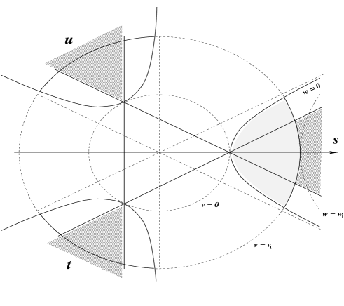
Figure 1: Central region of Mandelstam plane. The filled area bounded by curves $v=v_{1}$, $w=0$ is the expansion domain of the crossing invariant amplitudes $A^{\nu}(v,w)$.

We already know (see eq. (35)) that for such functions the Partial Wave Analysis (PWA) is identical in all physical regions. The coefficients $A^{L,N}_{\nu}$ of the PWA expansion

$$A_{\nu}(v,w)=(32\pi)\sum_{L={\rm even}}(2L+1)A_{\nu}^{L}({\bf k}^{2})P_{L}(\cos\Theta)\;;$$ (47)

$$A_{\nu}^{L}({\bf k}^{2})=\sum_{N=0}{\bf k}^{2(N+L)}A_{\nu}^{L,N}\;\;(\nu=0,1,2)\;$$ (48)

are easily calculated for every term of the expansion (45) by the formula

$$A_{\nu}^{L,N}=\frac{1}{64\pi}\frac{1}{(N+L)!}\left(\frac{d}{d({\bf k}^{2})}\right)^{N+L}\int_{-1}^{1}d\cos\Theta~{}P_{L}(\cos\Theta)A_{\nu}(v,w)~{}|_{{\bf k}=0}\;,$$ (49)

where expressions for variables $v$, $w$ in terms of ${\bf k}^{2}$, $\cos\Theta$ are given by relations (3), (34).

For 6 lowest terms of the expansion (45)

$$A^{\nu}(v,w)=(32\pi)(g^{\nu}_{00}+vg^{\nu}_{10}+wg^{\nu}_{01}+v^{2}g^{\nu}_{20}+vwg^{\nu}_{11}+w^{2}g^{\nu}_{02}+\dots)\;$$ (50)

the nonzero PWA parameters are

$$A_{\nu}^{0,0} = g^{\nu}_{00}\;;$$ (51)

$$A_{\nu}^{0,1} = 12(g^{\nu}_{10}-6g^{\nu}_{01})\;;$$ (52)

$$A_{\nu}^{0,2} = 2(72g^{\nu}_{20}-432g^{\nu}_{11}+5g^{\nu}_{10}+2592g^{\nu}_{02}-48g^{\nu}_{01})\;;$$ (53)

$$A_{\nu}^{0,3} = 12(20g^{\nu}_{20}-156g^{\nu}_{11}+1152g^{\nu}_{02}-3g^{\nu}_{01})\;;$$ (54)

$$A_{\nu}^{0,4} = 72(7g^{\nu}_{20}-96g^{\nu}_{11}+1008g^{\nu}_{02})/5\;;$$ (55)

$$A_{\nu}^{0,5} = 1728(-g^{\nu}_{11}+21g^{\nu}_{02})/5\;;$$ (56)

$$A_{\nu}^{0,6} = 7776g^{\nu}_{02}/5\;;$$ (57)

$$A_{\nu}^{2,0} = 2(g^{\nu}_{10}+12g^{\nu}_{01})/5\;;$$ (58)

$$A_{\nu}^{2,1} = 12(4g^{\nu}_{20}+12g^{\nu}_{11}-288g^{\nu}_{02}+3g^{\nu}_{01})/5\;;$$ (59)

$$A_{\nu}^{2,2} = 288(g^{\nu}_{20}+12g^{\nu}_{11}-234g^{\nu}_{02})/35\;;$$ (60)

$$A_{\nu}^{2,3} = 432(5g^{\nu}_{11}-132g^{\nu}_{02})/35\;;$$ (61)

$$A_{\nu}^{2,4} = -15552g^{\nu}_{02}/35\;;$$ (62)

$$A_{\nu}^{4,0} = 8(g^{\nu}_{20}+12g^{\nu}_{11}+144g^{\nu}_{02})/35\;;$$ (63)

$$A_{\nu}^{4,1} = 144(g^{\nu}_{11}+24g^{\nu}_{02})/35\;;$$ (64)

$$A_{\nu}^{4,2} = 2592g^{\nu}_{02}/35\;.$$ (65)

It is reasonable to consider the coefficients $A_{\nu}^{L,N}$ as the subsidiary phenomenological parameters. These parameters are directly related to the ordinary threshold parameters of the $\pi\pi$ amplitude entering eq. (21). For partial waves of isospin amplitudes

$$T^{I=0}=3A+B+C=5A_{0}+4\theta_{R}A_{1}+2[(2\theta_{R})^{2}+3V]A_{2}\;;$$ (66)

$$T^{I=1}=-B+C=-2\sqrt{3}\theta_{I}\{A_{1}-2\theta_{R}A_{2}\}\;;$$ (67)

$$T^{I=2}=B+C=2A_{0}-2\theta_{R}A_{1}-[(2\theta_{R})^{2}-6V]A_{2}\;$$ (68)

one can find the following relations:

$$T_{L}^{I=0} = 5A_{0}^{L}+4\theta_{R}A_{1}^{L}+2\left[5\theta_{R}^{2}+9{\bf k}^{4}\frac{2L^{2}+2L-1}{(2L-1)(2L+3)}\right]A_{2}^{L}$$ (69)

$$+18{\bf k}^{4}\left[\frac{L-1}{2L-1}\frac{L}{2L+1}A_{2}^{L-2}+\frac{L+1}{2L+1}\frac{L+2}{2L+3}A_{2}^{L+2}\right]\;;$$

$$T_{L}^{I=1}=\sqrt{3}{\bf k}^{2}\left[\frac{L}{2L+1}(A_{1}^{L-1}-2\theta_{R}A_{2}^{L-1})+\frac{L+1}{2L+1}(A_{1}^{L+1}-2\theta_{R}A_{2}^{L+1})\right]\;;$$ (70)

$$T_{L}^{I=2} = 2A_{0}^{L}-2\theta_{R}A_{1}^{L}+2\left[\theta_{R}^{2}+9{\bf k}^{4}\frac{2L^{2}+2L-1}{(2L-1)(2L+3)}\right]A_{2}^{L}$$ (71)

$$+18{\bf k}^{4}\left[\frac{L-1}{2L-1}\frac{L}{2L+1}A_{2}^{L-2}+\frac{L+1}{2L+1}\frac{L+2}{2L+3}A_{2}^{L+2}\right]\;.$$

In the above expressions whenever the partial–wave index $L$ of $A_{\nu}^{L}$ becomes less then zero the value of $A_{\nu}^{L}$ must be set to zero. Here, for the purpose of brevity the expression (29) for $\theta_{R}=\theta_{R}({\bf k}^{2})$ had not been expanded.

The low energy parameters (21) are then directly expressed in terms of quantities $\{A_{\nu}^{L,N}\}$ and, finally, in terms of the independent phenomenological parameters $g_{mn}^{\nu}$ of eq. (45). Leaving only the linear terms of the expansion (50) we get:

$${\bf[0]}\hskip 14.22636pta^{I=0}_{0,0} = 5g^{0}_{00}-8g^{1}_{00}{\mu}^{2}+56g^{2}_{00}{\mu}^{4}\;;$$ (72)

$${\bf[1]}\hskip 14.22636pta^{I=0}_{0,1} = 12(5g^{0}_{10}{\mu}^{2}-30g^{0}_{01}{\mu}^{4}-8g^{1}_{10}{\mu}^{4}+48g^{1}_{01}{\mu}^{6}-g^{1}_{00}+56g^{2}_{10}{\mu}^{6}$$ (73)

$$-336g^{2}_{01}{\mu}^{8}+14g^{2}_{00}{\mu}^{2})\;;$$

$${\bf(2)}\hskip 14.22636pta^{I=0}_{0,2} = 2(25g^{0}_{10}-240g^{0}_{01}{\mu}^{2}-112g^{1}_{10}{\mu}^{2}+816g^{1}_{01}{\mu}^{4}+1288g^{2}_{10}{\mu}^{4}$$ (74)

$$-8736g^{2}_{01}{\mu}^{6}+66g^{2}_{00})\;;$$

$${\bf(3)}\hskip 14.22636pta^{I=0}_{0,3} = 12(-15g^{0}_{01}-10g^{1}_{10}+120g^{1}_{01}{\mu}^{2}+272g^{2}_{10}{\mu}^{2}-2304g^{2}_{01}{\mu}^{4})\;;$$ (75)

$${\bf(4)}\hskip 14.22636pta^{I=0}_{0,4} = 144(15g^{1}_{01}+46g^{2}_{10}-648g^{2}_{01}{\mu}^{2})/5\;;$$ (76)

$${\bf(5)}\hskip 14.22636pta^{I=0}_{0,5} = -23328g^{2}_{01}/5\;;$$ (77)

$${\bf[2]}\hskip 14.22636pta^{I=0}_{2,0} = 2(5g^{0}_{10}+60g^{0}_{01}{\mu}^{2}-8g^{1}_{10}{\mu}^{2}-96g^{1}_{01}{\mu}^{4}+56g^{2}_{10}{\mu}^{4}$$ (78)

$$+672g^{2}_{01}{\mu}^{6}+6g^{2}_{00})/5\;;$$

$${\bf(3)}\hskip 14.22636pta^{I=0}_{2,1} = 12(15g^{0}_{01}-2g^{1}_{10}-48g^{1}_{01}{\mu}^{2}+40g^{2}_{10}{\mu}^{2}+432g^{2}_{01}{\mu}^{4})/5\;;$$ (79)

$${\bf(4)}\hskip 14.22636pta^{I=0}_{2,2} = 144(-21g^{1}_{01}+19g^{2}_{10}+396g^{2}_{01}{\mu}^{2})/35\;;$$ (80)

$${\bf(5)}\hskip 14.22636pta^{I=0}_{2,3} = 31104g^{2}_{01}/35\;;$$ (81)

$${\bf(4)}\hskip 14.22636pta^{I=0}_{4,0} = 48(g^{2}_{10}+12g^{2}_{01}{\mu}^{2})/35\;;$$ (82)

$${\bf(5)}\hskip 14.22636pta^{I=0}_{4,1} = 864g^{2}_{01}/35\;;$$ (83)

$${\bf[1]}\hskip 14.22636pta^{I=1}_{1,0} = 2(-g^{1}_{00}+4g^{2}_{00}{\mu}^{2})\;;$$ (84)

$${\bf[2]}\hskip 14.22636pta^{I=1}_{1,1} = 12(-2g^{1}_{10}{\mu}^{2}+12g^{1}_{01}{\mu}^{4}+8g^{2}_{10}{\mu}^{4}-48g^{2}_{01}{\mu}^{6}+g^{2}_{00})\;;$$ (85)

$${\bf(3)}\hskip 14.22636pta^{I=1}_{1,2} = 36(-3g^{1}_{10}+24g^{1}_{01}{\mu}^{2}+32g^{2}_{10}{\mu}^{2}-216g^{2}_{01}{\mu}^{4})/5\;;$$ (86)

$${\bf(4)}\hskip 14.22636pta^{I=1}_{1,3} = 216(g^{1}_{01}+3g^{2}_{10}-28g^{2}_{01}{\mu}^{2})/5\;;$$ (87)

$${\bf(5)}\hskip 14.22636pta^{I=1}_{1,4} = -1296g^{2}_{01}/5\;;$$ (88)

$${\bf[3]}\hskip 14.22636pta^{I=1}_{3,0} = 36(-g^{1}_{10}-12g^{1}_{01}{\mu}^{2}+4g^{2}_{10}{\mu}^{2}+48g^{2}_{01}{\mu}^{4})/35\;;$$ (89)

$${\bf(4)}\hskip 14.22636pta^{I=1}_{3,1} = 216(-3g^{1}_{01}+g^{2}_{10}+24g^{2}_{01}{\mu}^{2})/35\;;$$ (90)

$${\bf(5)}\hskip 14.22636pta^{I=1}_{3,2} = 3888g^{2}_{01}/35\;;$$ (91)

$${\bf[0]}\hskip 14.22636pta^{I=2}_{0,0} = 2(g^{0}_{00}+2g^{1}_{00}{\mu}^{2}+4g^{2}_{00}{\mu}^{4})\;;$$ (92)

$${\bf[1]}\hskip 14.22636pta^{I=2}_{0,1} = 6(4g^{0}_{10}{\mu}^{2}-24g^{0}_{01}{\mu}^{4}+8g^{1}_{10}{\mu}^{4}-48g^{1}_{01}{\mu}^{6}+g^{1}_{00}+16g^{2}_{10}{\mu}^{6}$$ (93)

$$-96g^{2}_{01}{\mu}^{8}+4g^{2}_{00}{\mu}^{2})\;;$$

$${\bf(2)}\hskip 14.22636pta^{I=2}_{0,2} = 4(5g^{0}_{10}-48g^{0}_{01}{\mu}^{2}+28g^{1}_{10}{\mu}^{2}-204g^{1}_{01}{\mu}^{4}+92g^{2}_{10}{\mu}^{4}$$ (94)

$$-624g^{2}_{01}{\mu}^{6}+6g^{2}_{00})\;;$$

$${\bf(3)}\hskip 14.22636pta^{I=2}_{0,3} = 12(-6g^{0}_{01}+5g^{1}_{10}-60g^{1}_{01}{\mu}^{2}+44g^{2}_{10}{\mu}^{2}-360g^{2}_{01}{\mu}^{4})\;;$$ (95)

$${\bf(4)}\hskip 14.22636pta^{I=2}_{0,4} = 72(-15g^{1}_{01}+17g^{2}_{10}-216g^{2}_{01}{\mu}^{2})/5\;;$$ (96)

$${\bf(5)}\hskip 14.22636pta^{I=2}_{0,5} = -3888g^{2}_{01}/5\;;$$ (97)

$${\bf[2]}\hskip 14.22636pta^{I=2}_{2,0} = 4(g^{0}_{10}+12g^{0}_{01}{\mu}^{2}+2g^{1}_{10}{\mu}^{2}+24g^{1}_{01}{\mu}^{4}+4g^{2}_{10}{\mu}^{4}$$ (98)

$$+48g^{2}_{01}{\mu}^{6}+3g^{2}_{00})/5\;;$$

$${\bf(3)}\hskip 14.22636pta^{I=2}_{2,1} = 12(6g^{0}_{01}+g^{1}_{10}+24g^{1}_{01}{\mu}^{2}+16g^{2}_{10}{\mu}^{2})/5\;;$$ (99)

$${\bf(4)}\hskip 14.22636pta^{I=2}_{2,2} = 72(21g^{1}_{01}+17g^{2}_{10}+36g^{2}_{01}{\mu}^{2})/35\;;$$ (100)

$${\bf(5)}\hskip 14.22636pta^{I=2}_{2,3} = 3888g^{2}_{01}/35\;;$$ (101)

$${\bf(4)}\hskip 14.22636pta^{I=2}_{4,0} = 48(g^{2}_{10}+12g^{2}_{01}{\mu}^{2})/35\;;$$ (102)

$${\bf(5)}\hskip 14.22636pta^{I=2}_{4,1} = 864g^{2}_{01}/35\;.$$ (103)

These relations establish the connection between the standard low energy parameters which are nonzero in the linear in $v$, $w$ approximation for all invariant functions $A_{\nu}$ and the real part of the phenomenological amplitude defined by eqs. (44), (45). Here, the bold–face numbers in the LHS show the order in ${\bf k}^{2}$; the numbers in the square brackets refer to the quantities which do not undergo corrections when three rest terms of the expansion (50) (as well as all higher order terms) are added.

Before introducing the form for the imaginary part let us briefly discuss the specific features of the considered ansatz.

First, one can find that 3 lowest scattering lengths $a^{I=0}_{0,0}$, $a^{I=1}_{1,0}$, $a^{I=2}_{0,0}$ appear to be unconstrained already in the zero approximation. (For simplicity we do not count the powers coming from structural combinations $({\theta}+\bar{\theta})$, $({\theta}+\bar{\theta})^{2}$, etc. in eqs. (44).) The linear approximation with 9 phenomenological parameters determine the quantities which by an accident are also 9 in total (those marked with order value given in the square brackets). The rest scattering lengths and slopes can not be free: their total number is growing twice faster than the number of free phenomenological parameters. The analysis of relations (69), (70), (71) makes it evident that the standard low energy characteristics $a^{I}_{L,N}$ of the expansion (21) are in the one–to–one correspondence with the subsidiary parameters $A^{L,N}_{\nu}$ of the crossing invariant amplitudes $A_{\nu}$. Therefore, it is the PWA expansion (47) where parameters $A^{L,N}_{\nu}$ can not be arbitrary: an inspection of the relations (51)–(65) might illustrate this. In the general case, bringing an expansion of the kind (47) back to the form (38) of the previous section one must obtain the vanishing coefficients at $({\theta}+\bar{\theta})$ and $({\theta}+\bar{\theta})^{2}$ structures because of the crossing invariance of the considered function. Being expressed via subsidiary parameters $A^{L,N}_{\nu}$ and, finally, via scattering lengths and slopes these two vanishing coefficients provide two infinite sets of conditions for the low energy characteristics of the $\pi\pi$ amplitude.

In the present work we do not plan to discuss in more details the arising conditions. We only would like to state that the conditions definitely differ from Roy equations [14] since only the threshold characteristics are being involved.

Second, one can derive more strong conclusions when invoking the properties of the $\pi\pi$ scattering implied by ChPT. This time the structure $({\theta}+\bar{\theta})$ ($({\theta}+\bar{\theta})^{2}$) must be considered as the $O(k^{2})$ ($O(k^{4})$) quantity. What is more important it is the increased ChPT weight of basic variables: $v\sim O(k^{4})$, $w\sim O(k^{6})$. This results in the different counting scheme which, for example, at $O(k^{6})$ leaves in effect only the following parameters of the considered approximation:

$$\begin{array}[]{ccccl}O(k^{0})\;:&g^{0}_{00}&&&;\\ O(k^{2})\;:&&g^{1}_{00}&&;\\ O(k^{4})\;:&g^{0}_{10}&&g^{2}_{00}&;\\ O(k^{6})\;:&g^{0}_{01}&g^{1}_{10}&&.\end{array}$$ (104)

Since no dynamics was used in the above pure kinematical considerations the actual scheme might be even more constrained. For example, to make the amplitude vanish in the chiral limit the value of $g^{0}_{00}$ must be of the order $O(\mu^{2})$. (In the leading order of ChPT one has $g^{0}_{00}=\mu^{2}/(3F^{2}_{\pi})$, $g^{1}_{00}=-2/(3F^{2}_{\pi})$.)

However, to provide the model–independent test of ChPT predictions one should not rely upon the above scheme. This does not mean that one inavoidably has to proceed with the third order expansion (45) for testing the two–loop results. Since the latter are given as corrections to the quantities of the lower order the linear approximation in the expansion (45) is sufficient both for testing the two–loop calculations and for confronting the standard and the generalized ChPT predictions [13, 11].

At last, one must note the rather large degree of slope parameters and higher scattering lengths which are necessary to be present in the amplitude to ensure the balance of the crossing properties — this is illustrated by relations (51)–(65), (72)–(103). The neglect of such a parameter, if at all possible without prescribing definite value for a lower one, causes the appearance of higher terms in the expansion (45) for the compensation.

To finish the amplitude development we must consider the imaginary part. The simple model (41), (42) of the previous section provides an illustration of the fact that there are no constraints on expansion coefficients of the imaginary part originating from the pure crossing symmetry. On the other hand the imaginary part is known to be completely determined by the unitarity conditions provided the real part of the amplitude is given (cf. eq. (22)). Since the applicability of the perturbative solution of unitarity (20) is limited by the condition $|{\rm Re}~{}T^{I}_{L}|\approx|{\rm Im}~{}T^{I}_{L}|$ and the only known phase shift satisfying $\tan~{}\delta^{I}_{L}\approx\pm\pi/4$ is the $\delta^{I=0}_{0}$ one (at $s\approx(4\mu)^{2}$) we are safe to derive coefficients of the expansion (23) from eq. (22) below the inelastic threshold in the domain (1). The straightforward calculation results in the following expressions:

$$\beta^{I=0,2}_{0,0} = (a^{I}_{0,0})^{2}\;;$$ (105)

$$\beta^{I=0,2}_{0,1} = a^{I}_{0,0}(2a^{I}_{0,1}{\mu}^{2}+(a^{I}_{0,0})^{3})/{\mu}^{2}\;;$$ (106)

$$\beta^{I=0,2}_{0,2} = (2a^{I}_{0,2}a^{I}_{0,0}{\mu}^{4}+(a^{I}_{0,1})^{2}{\mu}^{4}+4a^{I}_{0,1}(a^{I}_{0,0})^{3}{\mu}^{2}+2(a^{I}_{0,0})^{6}-(a^{I}_{0,0})^{4})/{\mu}^{4}\;;$$ (107)

$$\beta^{I=0,2}_{0,3} = (2a^{I}_{0,3}a^{I}_{0,0}{\mu}^{6}+2a^{I}_{0,2}a^{I}_{0,1}{\mu}^{6}+4a^{I}_{0,2}(a^{I}_{0,0})^{3}{\mu}^{4}+6(a^{I}_{0,1})^{2}(a^{I}_{0,0})^{2}{\mu}^{4}$$ (108)

$$+12a^{I}_{0,1}(a^{I}_{0,0})^{5}{\mu}^{2}-4a^{I}_{0,1}(a^{I}_{0,0})^{3}{\mu}^{2}+5(a^{I}_{0,0})^{8}-4(a^{I}_{0,0})^{6}+(a^{I}_{0,0})^{4})/{\mu}^{6}\;;$$

$$\beta^{I=1}_{1,0} = (a^{I}_{1,0})^{2}\;;$$ (109)

$$\beta^{I=1}_{1,1} = 2a^{I}_{1,1}a^{I}_{1,0}\;.$$ (110)

Here, we limited ourselves by few terms because higher waves are heavily suppressed at the threshold (cf. eq. (23)). As a result all parameters $\beta^{I}_{L}$ of the imaginary part via relations (72), (103) are determined in terms of the phenomenological parameters $g_{mn}^{\nu}$ of the expansion (45); the expressions do not contain kinematics and allow fast fitting procedures when quantities $\beta^{I}_{L}$ are used as formal (dependent) parameters.

This construction determines the imaginary parts of amplitudes $T^{I}$ with the fixed isospin of the decomposition (5) in the $s$–channel physical region. The isoscalar amplitudes in the same domain as well as any amplitude of a specific process are then simply determined by inverting the relations (8). This completes the construction of the phenomenological $\pi\pi$ amplitude suitable for the analysis of experimental data in the low energy region.

5 Conclusions

We derived the general model–independent form of the real part of the $\pi\pi$ amplitude near the threshold basing on the nice invariance properties of the variables $v,w$ under the crossing transformations and the independence of the basic crossing–covariant variables ${\theta}$, $\bar{\theta}$. The expansion which we elaborated contains an equivalent of the threshold characteristics (scattering lengths and slopes) in an explicitly crossing covariant terms and it is valid for the threshold regions of all 3 cross channels ($s,t,u$) simultaneously.

The advantage of the approach might be clearly displayed by a comparison with the analysis by Roskies [19] which is based on the ordinary Mandelstam variables $s,t,u$ and is valid for the central point $s=t=u=4\mu^{2}/3$. The sophisticated solution of the crossing restrictions in Mandelstam variables is given there in terms of the orthogonal polynomials over the central triangle of the Mandelstam plane [20]. The origin of the difference stems from the fact that in terms of the ordinary variables it is possible to construct only one crossing–invariant amplitude (namely, $(A+B+C)/3=A^{0}+2VA^{2}$).

Unfortunately, because of large errors of the existing data on the low energy $\pi\pi$ scattering now it is not possible to fix with the satisfactory precision the model–independent phenomenological parameters of our amplitude (44), (45). For example, only four parameters are sufficient to fit (with $\chi^{2}/N_{\rm DF}=0.10$) the data on scattering lengths and slopes of the compilation [21] providing (in the pion–mass units)

$$g^{0}_{00}= \;\;0.024\pm 0.005\;\;\;;\;\;g^{0}_{10}= 0.00124\pm 0.00025\;;$$

$$g^{1}_{00}= -0.0178\pm 0.0008\;;\;\;g^{2}_{00}= -0.00031\pm 0.00015\;.$$ (111)

Thus it is instructive to compare directly the theoretical amplitudes themselves, namely, the ChPT one–loop amplitude $A_{\rm GL}$ of the papers [2] with that given by eqs. (44), (45) in the $O({\bf k}^{4})$ order. Minimizing the expression

$$\Delta=\frac{\int_{4}^{8}ds\sigma(s)\int_{4-s}^{0}dt\left|A-A_{\rm GL}\right|^{2}}{\int_{4}^{8}ds\sigma(s)\int_{4-s}^{0}dt\left|A_{\rm GL}\right|^{2}}\;,$$ (112)

with the four–parameter amplitude one gets $\Delta\simeq 0.0090$. This is quite below the level of the accuracy as of the existing data as well as of the data which are being awaited in the near future [10]. For simplicity only the real phenomenological amplitude was used. Since more realistic amplitude as well as the one of the higher ChPT order will have the imaginary part which might be only few times larger, the value of $\Delta$ presents, in fact, an estimate to what extent the parameters (105)–(110) of the imaginary part are effective in the Mandelstam domain (1).

A brief summary of the most important properties of the discussed phenomenological amplitude includes:

1. The Lorentz invariance of expressions determining the amplitude in terms of the independent parameters (in contrast to the explicit Reference–Frame dependence of the standard set in the definition (21) which complicates the application to processes like $\pi N\to\pi\pi N$, $\gamma N\to\pi\pi N$ where the CMF of the dipion system does not coincide with the CMF of the reaction and, moreover, is “moving” from point to point of the phase space).

2. The explicit crossing covariance and the universal description of the threshold regions of all 3 cross channels.

3. Easy (perturbative) unitarity corrections which at the threshold always come in the higher order.

Therefore, the presented phenomenological $\pi\pi$ amplitude is suitable for the analysis of the $K\to\pi\pi e{\nu}$ decay and the $\pi N\to\pi\pi N$ reaction from the threshold $P_{\rm l.s.}=280$Mev/c up to $P_{\rm l.s.}\simeq 500$Mev/c since the energy region $s_{\pi\pi}\sim 8\mu^{2}$ is statistically insignificant or unreachable in the above conditions. The results then might find the application for the determination of the axial anomaly (when processing the final–state interaction corrections to the $\gamma\to 3\pi$ vertex of the amplitude of $\gamma N\to\pi\pi N$ reactions) and in other similar cases.

This research was supported in part by the RFBR grant N 95-02-05574a.

References

• [1] S. Weinberg. Physica 96A (1979) 327.
• [2] J. Gasser and H. Leutwyler. Ann. Phys. (NY) 158 (1984) 142; Nucl. Phys. B250 (1985) 465.
• [3] M.K. Volkov and V.N. Pervushin. Yad. Fyz. 20 (1974) 762; Yad. Fyz. 22 (1975) 366; Nuovo Cim. A27 (1975) 277.
• [4] M.K. Volkov and V.N. Pervushin. Essentially nonlinear quantum theories, dynamical symmetries and physics of mesons. Atomizdat, Moscow, 1978, 240p. (in russian).
• [5] B.R. Martin, D. Morgan and G. Shaw. Pion–Pion Interactions in Particle Physics. Academic Press, NY, 1976.
• [6] A.A. Bel‘kov, K.N. Mukhin and O.O. Patarakin. Pion–Pion Interactions. Energoatomizdat, Moscow, 1985.
• [7] J.F. Donoghue, E. Golowich and B. Holstein. Dynamics of the Standard Model. Cambridge University Press, NY, 1992.
• [8] Ulf–G. Meissner. Rep. Prog. Phys. 56 (1993) 903.
• [9] A. Pich. Rep. Prog. Phys. 58 (1995) 563.
• [10] D. Pocanic. Summary of $\pi$ $\pi$ Scattering Experiments, in A.M. Bernstein and B.R. Holstein (eds.), Chiral Dynamics: Theory and Experiment, Proceedings of the Workshop held at MIT, Cambridge, MA, USA, 25–29 July 1994, Lecture Notes in Physics, LNP 452 (Springer–Verlag, Berlin and Heidelberg, 1995), p. 95.
• [11] M. Knecht, B. Moussalam, J. Stern and N.H. Fuchs. Nucl. Phys. B457 (1995) 513.
• [12] J. Stern, H. Sazdjian and N.H. Fuchs. Phys. Rev. D47 (1993) 3814.
• [13] J. Bijenes, G. Colangelo, G. Ecker, J. Gasser and M.A. Sainio. Phys. Lett. B374 (1996) 210.
• [14] S.M. Roy. Phys. Lett. 36B (1971) 353; S.D. Protopopescu et al. Phys. Rev. D7 (1973) 1979; E.A. Alekseeva et al. ZETP 82 (1982) 1007.
• [15] O.O. Patarakin, V.N. Tikhonov and K.N. Mukhin. Nucl. Phys. A598 (1996) 335.
• [16] A.A. Bolokhov, S.G. Sherman, V.V. Vereshagin. Sov. Journ. Nucl. Phys. 46 (1987) 585.
• [17] A.A. Bolokhov, V.V. Vereshagin and S.G. Sherman. Nucl. Phys. A530 (1991) 660.
• [18] S.Mandelstam. Nuovo Cim. 15 (1960) 658.
• [19] R. Roskies. Crossing Restrictions on $\pi\pi$ Partial Waves. Preprint Ref.TH.1067-CERN (1969).
• [20] A.P. Balachandran and J. Nuyts. Phys. Rev. 172 (1968) 1821.
• [21] O. Dumbrais et al. Nucl. Phys. B216 (1983) 277.