HD-THEP-96-56

hep-ph/9612364

December 14, 1996

The 2-loop MSSM finite temperature effective potential with stop condensation

D. Bödeker, P. John, M. Laine and M.G. Schmidt

Institut für Theoretische Physik, Philosophenweg 16, D-69120 Heidelberg, Germany

Abstract

We calculate the finite temperature 2-loop effective potential in the MSSM with stop condensation, using a 3-dimensional effective theory. We find that in a part of the parameter space, a two-stage electroweak phase transition appears possible. The first stage would be the formation of a stop condensate, and the second stage is the transition to the standard electroweak minimum. The two-stage transition could significantly relax the baryon erasure bounds, but the parameter space allowing it ($m_{H}\mathop{\raise 1.29167pt\hbox{$<$\kern-7.5pt\raise-4.73611pt\hbox{$\sim$}}}100$ GeV, $m_{\tilde{t}_{R}}\sim 155-160$ GeV) is not very large. We estimate the reliability of our results using renormalization scale and gauge dependence. Finally we discuss some real-time aspects relevant for the viability of the two-stage scenario.

1 Introduction

The electroweak (EW) phase transition in the early universe has been under intense investigation in recent years (for reviews, see [1, 2]). Indeed, the Standard Model (SM) offers the three necessary ingredients of Sakharov for baryogenesis [1, 3]. However, careful studies have shown that in the SM (i) it may be somewhat difficult to produce enough baryons during the EW phase transition, due to the limited amount of CP-violation available and (ii) even if a $B+L$ asymmetry is produced, it is washed out afterwards by the sphaleron effects. This is because the phase transition is only very weakly of first order for the experimentally allowed Higgs masses $m_{H}\mathop{\raise 1.29167pt\hbox{$>$\kern-7.5pt\raise-4.73611pt\hbox{$\sim$}}}60$ GeV, and even vanishes for $m_{H}\mathop{\raise 1.29167pt\hbox{$>$\kern-7.5pt\raise-4.73611pt\hbox{$\sim$}}}m_{W}$ [4].

Thus one has to return to speculative models of baryogenesis in the very early stages of the universe marked by grand unification and related topics — or one has to consider variants of the SM. The SM has been and still is incredibly successful in explaining experiments though its limited range is generally accepted. Supersymmetric extensions are today the only way to maintain perturbative calculability at higher scales and the practical success of the SM. Furthermore, from the theoretical point of view supersymmetry (SUSY) appears to be the only known attractive way of including quantum gravity through supersymmetric string theory. Still, SUSY has to be detected in experiments!

The most simple SUSY model is the minimal supersymmetric extension (MSSM) of the SM: here the only new particles proposed are the superpartners with known (SM) couplings and an additional Higgs doublet. This is a very strong restriction in view of the multitude of possibilities offered, e.g., by string theory, but even in this simple case the necessary soft SUSY breaking terms introduce a huge number of free parameters. Fortunately we are interested in the behaviour of such a model at the high temperatures of a (modified) EW phase transition, in which case the problem simplifies. The new fermionic superpartners, the gauginos and higgsinos, become even more massive in the heat bath and can be integrated out. They may be important, however, for introducing strong CP-violating effects. The scalar quark partners, if heavy enough, can also be integrated out. Then the remaining nonzero Matsubara modes and heavy zero modes contribute to a 3-dimensional (3d) effective action like in the standard case [5]. “Integrating out” in the above means matching parameters in the comparison of a 4d and 3d set of amplitudes as in [6, 7, 8]. The effective theory for the light modes contains Higgs and gauge fields. If some combination of the two Higgs doublets is heavy compared with the scale $g^{2}T$, it can also be integrated out, resulting in an effective action of the same general form as for the SM [7, 9, 10, 11]. This case leads to conclusions which are not much more optimistic than in the SM [9–14]: for generic parameters, the phase transition would be at most relatively weakly of first order for Higgs masses $m_{H}\mathop{\raise 1.29167pt\hbox{$>$\kern-7.5pt\raise-4.73611pt\hbox{$\sim$}}}60-70$ GeV.

However, recently it has been argued that a rather light ($m_{\tilde{t}_{R}}\mathop{\raise 1.29167pt\hbox{$<$\kern-7.5pt\raise-4.73611pt\hbox{$\sim$}}}m_{t}$) stop, the superpartner of the right-handed top, and low values of $\tan\beta$, allow for a strongly first-order phase transition even at Higgs masses $m_{H}\sim m_{W}$ [15, 16]. Furthermore, the influence of 2-loop contributions to the effective potential was observed to be large due to the strong interactions of the stop entering at the 2-loop level, strengthening the transition [17].

In this paper we investigate the MSSM with a light stop in some detail. In particular, we study the possibility of a two stage transition in which at some temperature the stop acquires a nonzero expectation value while the electroweak symmetry is still unbroken. In the second stage the universe would make a transition from the charge and colour breaking (CCB) minimum to the standard one. In Ref. [15] it was argued that a CCB minimum does not develop during the electroweak phase transition as long as $m_{\tilde{t}_{R}}$ satisfies the bound necessary for vacuum stability at zero temperature; here we demonstrate that stop condensation may be possible in some part of the parameter space after all, leading to a two-stage transition in which the standard EW minimum is the global one at low temperatures. Such a transition would relax the baryon erasure bounds and allow for large Higgs masses, $m_{H}\mathop{\raise 1.29167pt\hbox{$<$\kern-7.5pt\raise-4.73611pt\hbox{$\sim$}}}100$ GeV.

We compute the effective potential for the Higgs and stop fields at two loops in 3d, working in an arbitrary background gauge. The gauge and renormalization scale dependence of our results should give an estimate of the size of higher loop contributions. Finally, assuming that a two-stage transition takes place, we discuss some issues concerning the real-time history of such a transition. Previously, two-stage transitions (in two Higgs doublet models) have been considered in [18].

The plan of the paper is the following. In Sec. 2 we discuss the 3d effective theory describing the EW phase transition in the MSSM. Sec. 3 contains the derivation of the 2-loop effective potential in the 3d theory. Implications from the 2-loop potential for the phase diagram of MSSM are presented in Sec. 4. In Sec. 5 we address some real-time aspects of the finite temperature phase transitions found, and the conclusions are in Sec. 6. Some details related to Secs. 2, 3 are in the two appendices.

2 The effective 3d theory and its parameters

The effective 3d theory relevant for the EW phase transition in MSSM is [11]

$$L = {\frac{1}{4}}F^{a}_{ij}F^{a}_{ij}+{\frac{1}{4}}G^{A}_{ij}G^{A}_{ij}+(D_{i}^{w}H)^{\dagger}(D_{i}^{w}H)+m_{H3}^{2}H^{\dagger}H+\lambda_{H3}(H^{\dagger}H)^{2}$$ (2.1)

$$+ (D_{i}^{s}U)^{\dagger}(D_{i}^{s}U)+m_{U3}^{2}U^{\dagger}U+\lambda_{U3}(U^{\dagger}U)^{2}+\gamma_{3}H^{\dagger}HU^{\dagger}U.$$

Here $D_{i}^{w}=\partial_{i}-ig_{W3}\tau^{a}A_{i}^{a}/2$ and $D_{i}^{s}=\partial_{i}-ig_{S3}\lambda^{A}C_{i}^{A}/2$ are the SU(2) and SU(3) covariant derivatives, $g_{W3}$ and $g_{S3}$ are the corresponding 3d gauge couplings, $H$ is the Higgs doublet and $U$ is the right-handed stop field. This theory is an effective theory for the thermodynamics of the EW phase transition in MSSM, provided that the parameters are suitably fixed in terms of the temperature $T$ and the zero-temperature physical parameters of the theory [10, 11] (see also below). The theory in (2.1) should be particularly useful for the case that the right-handed stops are light, $m_{\tilde{t}_{R}}<m_{t}$, which has recently attracted a lot of attention since the EW phase transition appears then to be strong enough for baryogenesis [15, 16, 9, 11]. For a heavier stop, $m_{\tilde{t}_{R}}>m_{t}$, the $U$ field can be integrated out and the effective theory is just the 3d SU(2)$+$Higgs model as in the Standard Model [9, 10, 11].

The reasons why it may be convenient (even in perturbation theory) to study the theory (2.1) rather than to directly calculate the effective potential in 4d, are:

1. The use of (2.1) factorizes the problem into two parts. The first part, the derivation of (2.1), is purely perturbative and free of IR-problems. The second part is the analysis of (2.1) in 3d and is subject to the usual IR-problems at finite $T$. Thus the IR-problems can be studied in a simplified setting.

2. The effective theory (2.1) has a certain degree of universality, since the same 3d theory (with different parameter values) arises for many different 4d theories. Thus the IR-problems of many 4d theories can be studied once and for all using (2.1).

3. The construction of (2.1) automatically implements the daisy resummation procedure required for the mass parameters at finite temperature, as well as resummations for all the couplings appearing in the theory (establishing the scale at which they are to be evaluated). In addition, there are resummations related to heavy modes in 3d. Apart from the daisy resummation, these resummations are usually not implemented in direct calculations in 4d. Yet their effect may be numerically non-negligible: e.g., the finite temperature strong gauge coupling is much smaller than $g_{S}^{2}(m_{Z})T$.

4. One may eventually want to perform lattice simulations of the EW phase transition in the MSSM by using (2.1). Note that while the simulations in the Standard Model indicated that perturbation theory is surprisingly reliable for strong transitions [4, 19, 20], this may not necessarily hold in MSSM with two light scalar fields. In fact, we find that the renormalization scale and gauge dependence of the results is much larger than in the SM indicating that the convergence of the 2-loop perturbative expansion is worse. It should also be noted that there are always massless SU(3) gauge excitations related to an unbroken SU(2) subgroup in perturbation theory (even if the $U$-field has an expectation value), unlike in the SM. If lattice simulations are ever made, then it is useful to have perturbative results in the same theory for comparison.

These benefits are slightly shadowed by the fact that at present there is no accurate derivation of the parameters in (2.1) available for a wide range of 4d zero temperature parameters. While this derivation is straightforward and parallels the ones in [9, 10, 11], it is complicated by the fact that the whole mass spectrum of the MSSM enters through relatively large radiative corrections, especially in the strongly interacting sector. Moreover (as is discussed in more detail in Appendix A), the derivation should be made at 2-loop level as concerns the mass parameters, if one is studying a two-stage scenario where an accurate comparison of two critical temperatures is needed. This is because it is only a 2-loop calculation that fixes the scale appearing in the thermal screening terms ($\sim g_{S}^{2}T^{2}$). While a 2-loop derivation is quite doable [7], we will not go into it here. Instead we make a 1-loop derivation for a particular region of the parameter space, and an order of magnitude estimate of the 2-loop scale factors appearing. This derivation should illustrate with reasonable accuracy the real situation, and allows us to address some interesting problems:

1. In [15], it was found that a two-stage transition where the right-handed stop field ($U$) gets an expectation value should not be allowed, since then the CCB minimum would be the global one and one would remain there until the present day (a two-stage transition was argued to be ruled out in [21], as well, since it was found that there is no second order transition by which to get back to the standard EW minimum). Here we try to be somewhat more accurate in a particular region of the parameter space, and we demonstrate that a two-stage transition might be possible after all. While there remain uncertainties in our calculation and thus it is not clear whether this case is eventually realized, it is an interesting prospect and hence in our opinion worth studying.

2. In [17] it was found that for small right-handed stop masses, the 2-loop corrections in the effective potential for the $H$-direction are large, making the transition stronger. Here we calculate the 2-loop potential in a general $U,H$-background. We confirm the 2-loop effect found in [17], find similar large 2-loop corrections in the $U$-direction as well, and discuss the reliability of the statements based on these corrections. It should be stressed that the large 2-loop corrections are IR-sensitive 3d effects and thus independent of the 4d parameters used in the derivation of the effective theory.

Since the derivation of the parameters in (2.1) is a problem which completely factorizes from the calculation of the 2-loop effective potential in 3d, we will discuss this derivation separately in Appendix A. Let us here just summarize the zero temperature vacuum parameters used: the CP-odd Higgs mass $m_{A}$ is assumed for simplicity to be large ($m_{A}\mathop{\raise 1.29167pt\hbox{$>$\kern-7.5pt\raise-4.73611pt\hbox{$\sim$}}}300$ GeV), the squark mixing parameters are very small, the running top mass is $m_{t}\sim 170$ GeV and the left-handed squark mass parameter is relatively small, $m_{Q}\sim 300$ GeV. We then present the results as a function of $\tan\!\beta$ (or equivalently the Higgs mass $m_{H}$) and the right-handed stop mass $m_{\tilde{t}_{R}}$.

3 The 2-loop potential and physical observables

The effective theory (2.1) contains two fundamental representation Higgs fields: the Higgs doublet $H$ interacting via the electroweak SU(2) group, and the right-handed stop colour triplet $U$ interacting via the strong SU(3) group. We have calculated the 2-loop effective potential of this theory in a general $H,U$ background. After gauge fixing, there remains a global symmetry in the theory, so the effective potential only depends on

$$H^{\dagger}H\equiv\frac{\phi^{2}}{2},\quad U^{\dagger}U\equiv\frac{\chi^{2}}{2}.$$ (3.1)

In the 3d theory, the dimension of $\phi,\chi$ is GeV^1/2 after a trivial rescaling with $T$; we nevertheless often use for clarity the 4d dimensions, so that

$$\frac{\phi_{\rm 4d}}{T}=\frac{\phi_{\rm 3d}}{\sqrt{T}},$$ (3.2)

and similarly for $\chi$.

It should be noted that within the 3d theory (2.1), the temperature $T$ does not appear explicitly. It is hidden in the parameters of the 3d theory, for instance in $g_{S3}^{2}=g_{S}^{2}T$. All the dimensionful 3d observables could hence be expressed in terms of $g_{S3}^{2}$. However, to keep the connection to 4d physics clear and since the values of $g_{S3}^{2},T$ are numerically close to each other, we will rather express the results in terms of $T$.

We have calculated the effective potential $V(\phi,\chi)$ in a background field gauge with two gauge parameters, $\xi$ related to SU(2) and $\zeta$ related to SU(3). The applicability of the background field gauge to the present context has been discussed in [22]. We display our results in the Landau gauge $\xi,\zeta=0$, and other values of the gauge parameters are used in estimating the convergence of the calculation (see below). For generality, we have replaced SU(3) by SU($N$) in the calculation and we also keep a general dimension $d$ in the formulas before the evaluation of the final two integrals (B.35), (B.40), to which all others reduce. We work throughout in the $\overline{\mbox{\rm MS}}$ scheme with the scale parameter $\bar{\mu}$. The details of the calculation are in Appendix B.

From the effective potential we extract several gauge fixing independent physical quantities. The critical temperature $T_{c}^{\phi}$ for the transition from the origin to the standard electroweak (EW) minimum $\phi_{\rm min}$ is defined such that at $T_{c}^{\phi}$,

$$V(0,0)=V(\phi_{\rm min},0).$$ (3.3)

Similarly one finds the critical temperature $T_{c}^{\chi}$ for the transition from the origin to the charge and colour breaking (CCB) minimum $\chi_{\rm min}$ in the $U$ direction, and $T_{c}^{\chi\to\phi}$ for the transition from the CCB minimum to the EW minimum.

The strength of the phase transition with respect to the sphaleron rate is characterized by the vacuum expectation value $\phi_{\rm min}/T$ in the broken phase. This is a gauge dependent quantity; we calculate it in the Landau gauge. A gauge independent characterization of the discontinuity could be obtained with the expectation values of the composite operators $H^{\dagger}H,U^{\dagger}U$ [23]:

$$\Delta\langle H^{\dagger}H\rangle = \frac{d}{dm_{H3}^{2}}\biggl{[}V(\phi_{\rm min},0)-V(0,0)\biggr{]},$$

$$\Delta\langle U^{\dagger}U\rangle = \frac{d}{dm_{U3}^{2}}\biggl{[}V(0,\chi_{\rm min})-V(0,0)\biggr{]}.$$ (3.4)

However, numerically $\Delta\langle H^{\dagger}H\rangle\sim\phi_{\rm min}^{2}/2$, $\Delta\langle U^{\dagger}U\rangle\sim\chi_{\rm min}^{2}/2$, so that we do not separately discuss the quantities in (3.4).

The latent heat is defined by

$$L=T_{c}\frac{d}{dT}\left.\biggl{(}p_{h}(T)-p_{l}(T)\biggr{)}\right|_{T=T_{c}},$$ (3.5)

where $p_{h}(T)$ ($p_{l}(T)$) is the pressure $p(T)=-V({\rm min})$ in the high (low) temperature phase (note that we mostly write $V(\phi,\chi)$ in 4d units; the relation to 3d is $V_{\rm 4d}=TV_{\rm 3d}$, apart from field independent terms). For the surface tension we use the leading order expression

$$\sigma=\int_{\varphi_{1}}^{\varphi_{2}}\!d\varphi\,\sqrt{2[V(\varphi)-V(\varphi_{1})]},$$ (3.6)

where $\varphi=(\phi,\chi)$, $d\varphi$ is the length element in the field space, and the path is the one that minimizes the result (this can be derived by extremizing the bounce action at $T_{c}$). Perturbative corrections to the surface tension from the derivative terms in the SU(2)$+$Higgs model were discussed in [24, 25].

It is important to estimate the reliability of the perturbative results obtained. To this end, one can use the fact that the physical observables derived are gauge- and $\bar{\mu}$-independent to the order to which they have been calculated. The remaining dependence then gives an estimate of the magnitude of higher-order corrections. For the gauge dependence, we vary $\xi,\zeta$ from zero to $\sim 1$. For the $\bar{\mu}$-dependence, we compare results from the choice $\bar{\mu}=T$ with results from a renormalization group (RG) improved optimized choice [6]. The optimization condition is that the 2-loop contribution to $V^{\prime}(\varphi)$ vanishes, and it gives a field dependent scale parameter $\bar{\mu}(\varphi)$ which should be proportional to some (non-linear) combination of the mass scales contributing to $V(\varphi)$. The simple choice $\bar{\mu}=T$ is also supposed to reflect the mass scales of the problem, since the non-perturbative 3d masses should be of order $g_{W3}^{2},g_{S3}^{2}$ [4, 19, 26, 27, 28].

4 Numerical results

The 2-loop effective potential $V(\phi,\chi)$ for a particular choice of the parameters ($\tan\!\beta=5$, $m_{\tilde{t}_{R}}=158.3$ GeV, $\bar{\mu}=T$) at $T=T_{c}=92.43$ GeV is shown in Fig. 1. This choice corresponds to a special case in which there is a simultaneous first order transition in both directions. In general, the transitions take place at different temperatures $T_{c}^{\phi},T_{c}^{\chi}$, and there is a third temperature $T_{c}^{\chi\to\phi}$ at which the broken minima are at equal heights.

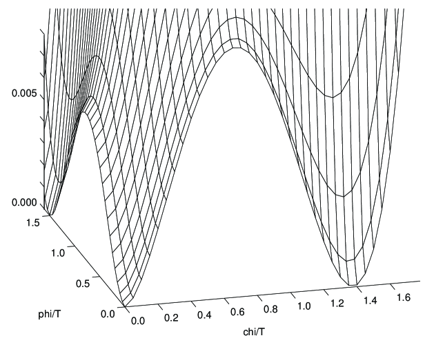
Figure 1: The 2-loop effective potential at $T=T_{c}^{\phi}=T_{c}^{\chi}=T_{c}^{\chi\to\phi}$ for $\tan\!\beta=5$ ($m_{H}\sim 92$ GeV), $m_{\tilde{t}_{R}}=158.3$ GeV, $\bar{\mu}=T$, $\xi=\zeta=0$.

The 2-loop potential corresponding to the parameters of Fig. 1 is displayed more precisely in the $\phi$- and $\chi$-directions in Fig. 2, together with the 1-loop potentials at the corresponding critical temperatures. One can observe several things. First, looking at the 1- and 2-loop potentials at the same $\bar{\mu}=T$, one sees that the 2-loop effects are large and seem to make the transition much stronger. For the $\phi$-direction this was observed in [17], and the reason for the strengthening was tracked down to 2-loop graphs involving the strongly interacting stops. From Fig. 2 one sees that there are similar large 2-loop corrections in the $\chi$-direction, as well.

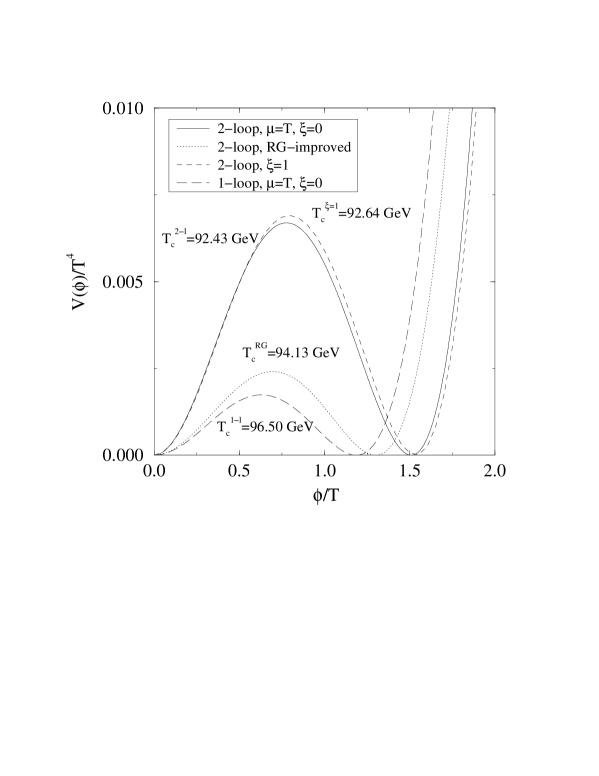
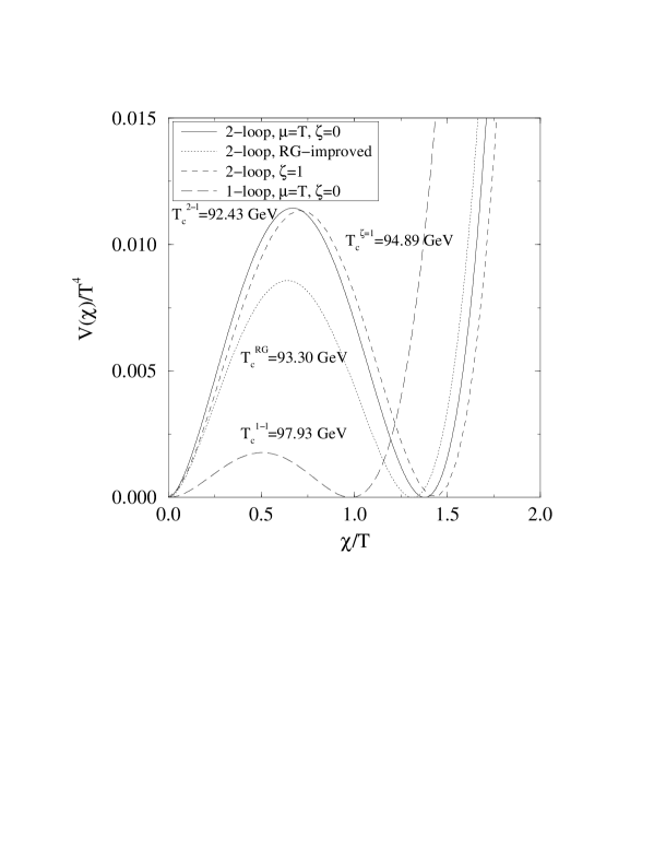
Figure 2: The 1-loop and 2-loop effective potentials at the corresponding critical temperatures, for $\tan\!\beta=5,m_{\tilde{t}_{R}}=158.3$ GeV. It is seen that there may be a relatively large uncertainty in the prediction for the surface tension due to the large $\bar{\mu}$-dependence, especially for the $\phi$-direction. The figure has been drawn at the special point $m_{\tilde{t}_{R}}=m_{\tilde{t}_{R},c}$ so that the critical temperatures $T_{c}^{\rm 2-l}$ of the two transitions are equal (see Fig. 3). The $\bar{\mu}$-dependence is especially large at this point, since the mass parameters $m_{H3}^{2}(\bar{\mu})$, $m_{U3}^{2}(\bar{\mu})$ are close to zero so that the relative change can be significant.

Second, comparing the 2-loop potentials at different choices of $\bar{\mu}$ ($\bar{\mu}=T$ vs. RG-improved $\bar{\mu}$), one can see that the reliability of the 2-loop results is questionable, especially for the $\phi$-direction. The large $\bar{\mu}$-dependence arises from the $\bar{\mu}$-dependence of $m_{U3}^{2}(\bar{\mu})$ (see Eq. (A.29)) in the 1-loop corrections, and would be cancelled by 3-loop graphs involving strong interactions. Thus the 3-loop contributions are quite important. The large $\bar{\mu}$-dependence seen here is in contrast to what has been observed in the pure SU(2)+Higgs model [6]. At the same time, even in the SU(2)+Higgs model non-perturbative results for the surface tension (which is characterized by the size of the bump between the minima, see (3.6)) were significantly smaller than 2-loop perturbative results for weaker transitions [4, 22]. Thus one can say that for the surface tension perturbative results are expected to give only an order of magnitude estimate. For the critical temperature the $\bar{\mu}$-dependence in Fig. 2 is somewhat smaller, so the existence of the two transitions and their crossing point is on a firmer basis. For the vevs and latent heats the $\bar{\mu}$-dependence is also relatively smaller than for the surface tension, so the perturbative estimates should produce the correct qualitative features.

The gauge dependence of $V(\phi,\chi)$ (obtained by varying $\xi,\zeta$ from zero to unity) is also shown in Fig. 2. It differs from the $\bar{\mu}$-dependence in being much larger in the $\chi$-direction, especially for $T_{c}$. The reason for the difference is that the $\bar{\mu}$-dependence arises from scalar (in particular stop) excitations affecting also the $\phi$-direction, whereas the gauge dependence arises from vector excitations. For quantities other than $T_{c}$ the gauge dependence appears to be smaller. It should be noted that the gauge dependence (as well as the $\bar{\mu}$-dependence) is significantly smaller at the 2-loop than at the 1-loop level. The error bars containing an estimate of both the 2-loop gauge and $\bar{\mu}$-dependence for the critical temperatures are shown in Fig. 3.

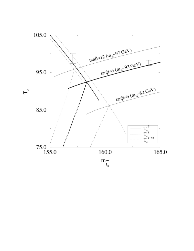
Figure 3: The critical temperatures of the three transitions as a function of $m_{\tilde{t}_{R}}$ for $\tan\!\beta=3,12$ (thin lines) and $\tan\!\beta=5$ (thick lines). The two-stage transition would take place to the left of the crossing point of the three critical curves; it is seen that a two-stage transition is possible, but there is not very much parameter space for it. The continuations of $T^{\phi}_{c}$ to the left of the crossing point, and $T^{\chi}_{c}$ to the right of it, roughly represent the region of metastability of the transition with a higher $T_{c}$. Error bars indicate the dependences on $\bar{\mu},\xi,\zeta$ (for $\tan\!\beta=5$), as explained in the text; the actual curves correspond to the Landau gauge and $\bar{\mu}=T$. In terms of the parameter $m_{U}^{2}=m_{\tilde{t}_{R}}^{2}-m_{t}^{2}$, the $x$-axis is from $-(70$ GeV)² to $-(40$ GeV)².

The dependence of the critical temperatures on $m_{\tilde{t}_{R}}$ and $\tan\!\beta$ is also shown in Fig. 3. The general pattern is the following: For a given $\tan\!\beta$, there is a certain critical value of $m_{\tilde{t}_{R}}$, for instance $m_{\tilde{t}_{R},c}=158.3$ GeV for $\tan\!\beta=5$. If $m_{\tilde{t}_{R}}>m_{\tilde{t}_{R},c}$, the critical temperature $T_{c}^{\phi}$ of the normal ($0\to\phi$) EW phase transition is higher than the critical temperature $T_{c}^{\chi}$ of the CCB transition ($0\to\chi$). In this case the EW phase transition proceeds in the normal way when the universe has cooled down to $T_{c}^{\phi}$. If $m_{\tilde{t}_{R}}<m_{\tilde{t}_{R},c}$, on the contrary, then $T_{c}^{\chi}>T_{c}^{\phi}$ and the universe ends up in the CCB minimum (provided that the first order phase transition is weak enough compared with the expansion rate of the universe). However, for the parameter values we are using, we find that the CCB minimum is not the global one at much lower temperatures. Instead, there is another first order phase transition at $T_{c}^{\chi\to\phi}<T_{c}^{\chi}$ in which the normal EW minimum becomes the global one. Thus, if this latter transition is weak enough to take place within the cosmological time scales available, one ends up finally in the normal EW minimum. The vacuum expectation value $\phi_{\rm min}$ can easily be large $\phi_{\rm min}/T_{c}\gg 1$ after the latter transition (Fig. 4), so that the sphaleron rate would be very effectively switched off.

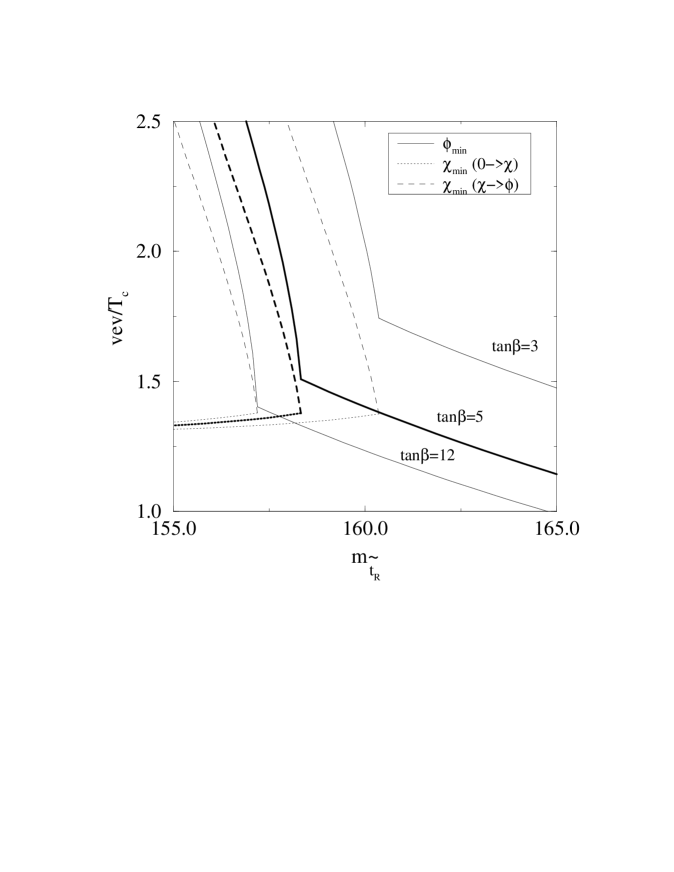
Figure 4: The expectation values $\phi_{\rm min}/T_{c}$, $\chi_{\rm min}/T_{c}$ of the three transitions (see Fig. 3) in the Landau gauge as a function of $m_{\tilde{t}_{R}}$ for $\tan\!\beta=3,5,12$. The broken phase transition from $\chi_{\rm min}>0$ to $\phi_{\rm min}>0$ is seen to easily lead to very large values of $\phi_{\rm min}$. For clarity the metastable branches are not shown here.

In Fig. 3 we have also shown the metastable branches of the EW ($0\to\phi$) and CCB ($0\to\chi$) transitions. These could be relevant if the transition with the higher $T_{c}$ is so strong that it has not taken place before the temperature has cooled down to the $T_{c}$ of the lower transition (see Sec. 5). When one goes far enough into the metastability region, then the higher transition definitely does take place since it would have reached the barrier temperature by the time of the lower $T_{c}$.

5 Real-time history

In the previous Section, we demonstrated that the phase diagram of the EW matter described by the MSSM may be such that the cosmological EW phase transition could take place in two stages. However, the transitions occurring would be of first order, so one has to discuss the amount of supercooling taking place and the possible reheating due to the latent heat released, as well, to see how the transitions would really proceed in the early universe. We will here make some simple estimates on the presumable real-time events.

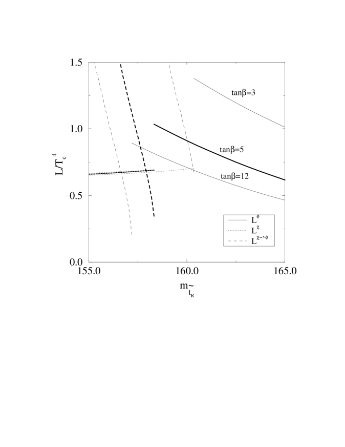
Figure 5: The latent heats of the transitions as a function of $m_{\tilde{t}_{R}}$ for $\tan\!\beta=3,5,12$. Note that at $m_{\tilde{t}_{R},c}$, $L^{\chi\to\phi}=L^{\phi}-L^{\chi}$. For smaller $m_{\tilde{t}_{R}}$, $L^{\chi\to\phi}$ grows rapidly. Metastable branches are not shown.

The parameters needed for the real-time estimates are the latent heat $L$ and the surface tension $\sigma$, scaled with powers of $T_{c}$: $\hat{L}\equiv L/T_{c}^{4}$, $\hat{\sigma}\equiv\sigma/T_{c}^{3}$. Indeed, the small supercooling formula [29, 30] for the nucleation temperature $\hat{T}_{n}=T_{n}/T_{c}$ is

$$1-\hat{T}_{n}\sim 0.4\frac{\hat{\sigma}^{3/2}}{\hat{L}},$$ (5.1)

assuming that in the high temperature phase $p(T)\propto T^{4}$. This formula can be expected to be valid only when $1-\hat{T}_{n}\ll 1$, and it usually breaks down by underestimating the value of $1-\hat{T}_{n}$. Another quantity of interest is the amount of heating that takes place after nucleation as the latent heat is released. Since the bubbles tend to fill the universe in a time scale very small compared with the time scale of expansion [24, 30], the reheating temperature $T_{r}$ can be estimated from

$$e_{h}(T_{n})=e_{l}(T_{r}),$$ (5.2)

where $e_{h}(T),e_{l}(T)$ are the energy densities in the high and low temperature phases, respectively. From (5.2) one finds that reheating to the critical temperature ($T_{r}>T_{c}$) takes place roughly if $\hat{L}\mathop{\raise 1.29167pt\hbox{$>$\kern-7.5pt\raise-4.73611pt\hbox{$\sim$}}}8\hat{\sigma}^{3/4}$, assuming that the effective number of massless degrees of freedom is $\sim 110$.

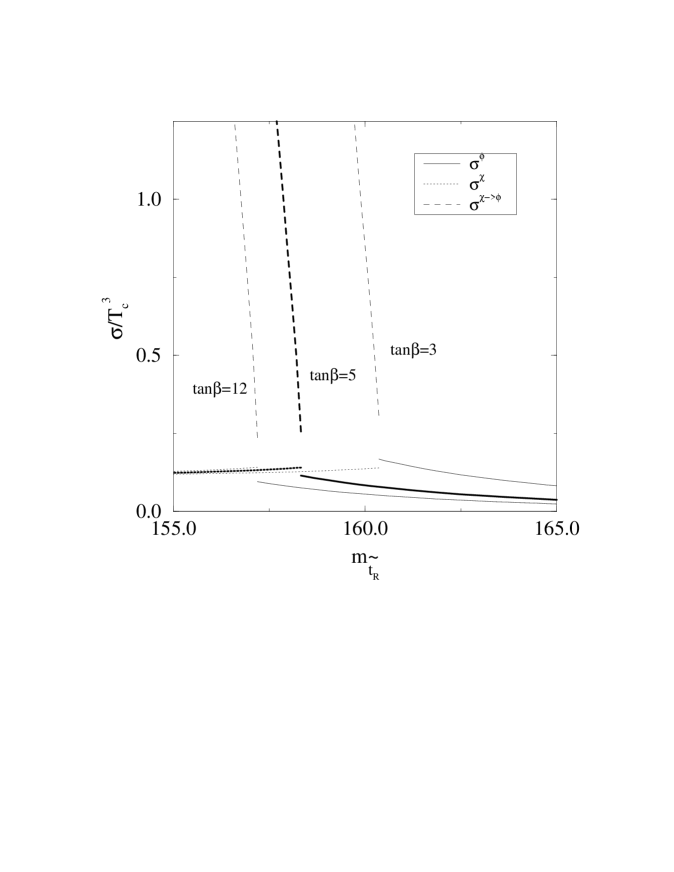
Figure 6: The surface tensions of the transitions as a function of $m_{\tilde{t}_{R}}$ for $\tan\!\beta=3,5,12$. The curves for the broken phase $\chi\to\phi$ transition represent an upper bound obtained as explained in the text. Note that at $m_{\tilde{t}_{R},c}$, $\sigma^{\chi\to\phi}=\sigma^{\phi}+\sigma^{\chi}$. It is seen that for the broken phase transition, the surface tension becomes rapidly very large. Metastable branches are not shown.

Results for the latent heat from (3.5) as a function of $\tan\!\beta,m_{\tilde{t}_{R}}$ are shown in Fig. 5.

To compute the surface tension (3.6) one has to find the path in $(\phi,\chi)$ space which minimizes the integral. Near $m_{\tilde{t}_{R}}=m_{\tilde{t}_{R},c}$ the mass parameters of the 3d theory are small. Then the effective potential is dominated by the term $\gamma_{3}\phi^{2}\chi^{2}/4$ in the tree level potential for $\phi,\chi\neq 0$ (see Fig. 1). Therefore the path which minimizes (3.6) for the transition $\chi\to\phi$ is close to the rectangular path which first goes from $(0,\chi_{\rm min})$ to $(0,0)$ and then from $(0,0)$ to $(\phi_{\rm min},0)$. We have used this path for estimating $\sigma^{\chi\to\phi}$ in Fig. 6. The corresponding values are therefore an upper limit for the surface tension. At lower critical temperatures $T_{c}^{\chi\to\phi}$, corresponding to smaller values of $m_{\tilde{t}_{R}}$, the 3d mass parameters decrease and our simple approximation becomes less reliable. We have used different trial paths and compared the results for $\sigma^{\chi\to\phi}$ with those from the rectangular path. From this we estimate the error as at most 10% for the parameter range shown in Fig. 6. This error estimate, of course, does not contain the effects of higher-loop and non-perturbative contributions, which might make $\sigma^{\chi\to\phi}$ much smaller.

Based on Figs. 5, 6 and on Eqs. (5.1), (5.2), one can say the following:

1. The EW ($0\to\phi$) and CCB ($0\to\chi$) transitions seem to proceed in the normal manner: there is at most a few percent supercooling, and the latent heat released after the nucleation period reheats the matter considerably. Especially for larger Higgs masses in the EW phase transition, one might even reheat back to $T_{c}^{\phi}$.

2. For the broken phase transition ($\chi\to\phi$), the supercooling is considerably larger. For instance, at the point $m_{\tilde{t}_{R},c}$ the latent heat is smaller ($L^{\chi\to\phi}=L^{\phi}-L^{\chi}$) and the surface tension is larger ($\sigma^{\chi\to\phi}=\sigma^{\phi}+\sigma^{\chi}$) than for the EW transition characterized by $L^{\phi},\sigma^{\phi}$. Both effects increase the supercooling. The small supercooling formula (5.1) gives numbers of the order of 10%, but the true supercooling might be even larger. Moreover, when one goes to smaller $m_{\tilde{t}_{R}}$ the surface tension seems to grow more rapidly than the latent heat, so that one may end up in a situation where the lifetime of the metastable CCB minimum is comparable with cosmological time scales. This is clearly unacceptable. There is also no barrier temperature for the broken phase transition [21]. Of course it might happen that some other nucleation mechanism enters, in which case the transition could proceed after all; or the non-perturbative surface tension might be much smaller than our simple estimate.

3. If one happens to be very close to $m_{\tilde{t}_{R},c}$, then things may become complicated. For instance, the supercooling for the CCB transition is generally somewhat larger than for the EW transition, so it is not excluded that at $m_{\tilde{t}_{R}}\mathop{\raise 1.29167pt\hbox{$<$\kern-7.5pt\raise-4.73611pt\hbox{$\sim$}}}m_{\tilde{t}_{R},c}$ one supercools so much that the metastable branch of $T_{c}^{\phi}$ in Fig. 3 becomes relevant. Then the EW transition might take place first. But after it has taken place, the CCB minimum is still the global one until $T=T_{c}^{\chi\to\phi}$, so that in principle two other transitions (first to the CCB minimum and then back to the EW minimum at $T<T_{c}^{\chi\to\phi}$) could occur. However, this possibility clearly requires fine tuning.

6 Discussion and conclusions

We have studied the electroweak phase transition in MSSM with $m_{\tilde{t}_{R}}<m_{t}$ at the 2-loop level of perturbation theory. It was found that in principle there is the possibility that the EW phase transition takes place in two stages. The first part, the colour breaking transition, would delay and strengthen the transition to the standard electroweak minimum. The sphaleron rate should not be significantly switched off in the colour breaking minimum since the $U$-field is an SU(2) singlet, but it would be very effectively switched off after the transition to the standard electroweak minimum for Higgs masses up to 100 GeV (in the standard minimum normal electroweak sphaleron estimates apply [31]). Our calculations were performed in a particular region of the parameter space, with a relatively large CP-odd Higgs mass $m_{A}$ and a relatively small left-handed third generation squark mass $m_{Q}\sim 300$ GeV, but it appears that relaxing these assumptions does not immediately change the qualitative pattern observed.

The problem with the two stage scenario is that the parameter region in $m_{\tilde{t}_{R}}$ allowing for a two stage transition is rather small, $m_{\tilde{t}_{R}}\sim 155-160$ GeV. There is always the danger that even though the CCB minimum becomes metastable, the first order transition to the standard EW minimum becomes so strong that the lifetime of the metastable state is comparable with cosmological time scales. Thus one may also interpret our result as a lower bound $m_{\tilde{t}_{R}}\mathop{\raise 1.29167pt\hbox{$>$\kern-7.5pt\raise-4.73611pt\hbox{$\sim$}}}155$ GeV for the right-handed stop mass. This particular number is valid for small squark mixing parameters.

Finally, it should be remembered that our study was based on 2-loop perturbation theory. In fact, already the large gauge and $\bar{\mu}$-dependence of our results indicates that higher-loop perturbative (and possibly non-perturbative) effects could be much larger than in the SU(2)+Higgs model which is relevant for the Standard Model and has been studied on the lattice. If the right-handed stop mass turns out to be such that the scenario studied could be realized, then one should probably consider lattice simulations in the 3d SU(3)$\times$SU(2) effective theory.

Appendix Appendix A

In this Appendix, we discuss in some detail how the parameters in (2.1) can be fixed at 1-loop (and partly 2-loop) level.

$T=0$ parameters

Since our main point is studying 3d IR phenomena and since an accurate derivation of the 3d theory with the whole MSSM mass spectrum included would be somewhat complicated, we will consider a rather simple special case here. The final effective theory (2.1) will be the same in many other cases as well, but the expressions for the parameters will be different. We consider the case of vanishing mixing in the squark mass matrix and a heavy CP-odd Higgs particle ($m_{A}\mathop{\raise 1.29167pt\hbox{$>$\kern-7.5pt\raise-4.73611pt\hbox{$\sim$}}}300$ GeV) so that only one Higgs doublet remains; this is the most favourable case for baryogenesis [14]. Neither of these assumptions affects the form of the final effective theory. For instance, for two Higgs doublets one can diagonalize the Higgs mass matrix close to $T_{c}$ and integrate the heavy doublet out [7, 9, 10, 11]. We mostly neglect the U(1) gauge coupling, which should be a good approximation with respect to the other uncertainties in the calculation. Finally, we assume that the only sparticles light enough to enter the calculation are the squarks in the third generation. Adding light fermionic degrees of freedom would again not change the form of the final effective theory, only its parameters (see [10] for the typical corrections arising).

We shall for definiteness consider a scenario with a relatively light left-handed squark mass parameter $m_{Q}\sim 300$ GeV. This is at the lower end of the phenomenological constraints obtained with a realistic top mass [13, 14], and at the same time still allows the high-temperature expansion for $T\sim 100$ GeV (we also take the right-handed sbottom mass parameter to be $m_{D}\sim 300$ GeV, although this has little effect). A much heavier $m_{Q}^{2}$ does not change the pattern we are investigating qualitatively, but the formulas to be used simplify as the $m_{Q}^{2}$-corrections decouple. The mass parameter $m_{U}^{2}$ is supposed to be relatively small, and its effects are discussed in the main text.

The most important renormalization effects of the $T=0$ vacuum theory with respect to our calculation concern the $\overline{\mbox{\rm MS}}$ mass parameters $m_{H}^{2}(\bar{\mu})$, $m_{U}^{2}(\bar{\mu})$ (we work throughout in the $\overline{\mbox{\rm MS}}$ scheme with the scale parameter $\bar{\mu}$). Calculating the pole Higgs mass $m_{H}$ to 1-loop order, one finds that $m_{H}^{2}(\bar{\mu})$ can be expressed in terms of physical quantities as

$$m_{H}^{2}(\bar{\mu})=-\frac{m_{H}^{2}}{2}+\frac{3}{16\pi^{2}}h_{t}^{2}\sin^{2}\!\beta\,m_{Q}^{2}\biggl{(}2\ln\frac{\bar{\mu}}{m_{\tilde{t}_{L}}}+1\biggr{)},$$ (A.1)

where only the dominant terms are kept. For instance, there is another term with $m_{Q}^{2}\to m_{U}^{2}$ and $m_{\tilde{t}_{L}}\to m_{\tilde{t}_{R}}$, but this is much less important for the parameter values we are considering. For the relation between $\tan\!\beta$ and $m_{H}$, we use the standard 1-loop formula containing the leading correction,

$$m_{H}^{2}=m_{Z}^{2}\cos^{2}\!2\beta+\frac{3g_{W}^{2}}{8\pi^{2}}\frac{m_{t}^{4}}{m_{W}^{2}}\ln\frac{m_{\tilde{t}_{R}}m_{\tilde{t}_{L}}}{m_{t}^{2}}.$$ (A.2)

Here, in the absence of mixing,

$$m_{\tilde{t}_{R}}^{2}=m_{U}^{2}+m_{t}^{2},\quad m_{\tilde{t}_{L}}^{2}=m_{Q}^{2}+m_{t}^{2}+{\frac{1}{2}}m_{Z}^{2}\cos\!2\beta\,.$$ (A.3)

We take $m_{t}=170$ GeV so that $m_{t}^{\rm pole}\sim 175$ GeV according to $m_{t}^{\rm pole}\sim m_{t}(1+\frac{4\alpha_{S}}{3\pi})$. The bottom Yukawa coupling is neglected.

Similarly, the dominant term in the expression for $m_{U}^{2}(\bar{\mu})$ is

$$m_{U}^{2}(\bar{\mu})=m_{U}^{2}+\frac{1}{8\pi^{2}}h_{t}^{2}m_{Q}^{2}\biggl{(}2\ln\frac{\bar{\mu}}{m_{\tilde{t}_{L}}}+1\biggr{)},$$ (A.4)

where $m_{U}^{2}$ is expressed in terms of physical masses through (A.3).

Step 1: dimensional reduction

Next we go to finite temperature. After integration over non-zero Matsubara frequencies, the effective theory for the thermodynamics of the electroweak phase transition contains only bosonic $n=0$ Matsubara modes [5–11,32]. The form of the effective theory can be written down immediately using 3d gauge invariance (only the terms coupled to $H,U,A^{a}_{i},C^{A}_{i}$ are shown explicitly below):

$$L = {\frac{1}{4}}F^{a}_{ij}F^{a}_{ij}+{\frac{1}{4}}G^{A}_{ij}G^{A}_{ij}+(D_{i}^{w}H)^{\dagger}(D_{i}^{w}H)+m_{H3}^{2}H^{\dagger}H+\lambda_{H3}(H^{\dagger}H)^{2}$$ (A.5)

$$+ (D_{i}^{s}U^{*})^{\dagger}(D_{i}^{s}U^{*})+m_{U3}^{2}U^{\dagger}U+\lambda_{U3}(U^{\dagger}U)^{2}+\gamma_{3}H^{\dagger}HU^{\dagger}U$$

$$+ (D^{ws}_{i}Q)^{\dagger}(D^{ws}_{i}Q)+(D^{s}_{i}D^{*})^{\dagger}(D^{s}_{i}D^{*})+m_{Q3}^{2}Q_{\alpha}^{\dagger}Q_{\alpha}+m_{D3}^{2}D_{\alpha}^{*}D_{\alpha}$$

$$+ h_{t3}^{2}\Bigl{(}Q^{*}_{i\alpha}U^{*}_{\alpha}Q_{i\beta}U_{\beta}+\sin^{2}\!\beta\,\tilde{H}^{\dagger}Q_{\alpha}Q^{\dagger}_{\alpha}\tilde{H}\Bigr{)}$$

$$+ {\frac{1}{4}}g_{W3}^{2}Q^{*}_{i\alpha}Q_{j\alpha}\Bigl{[}\sin^{2}\!\beta\,H^{*}_{k}H_{l}+\cos^{2}\!\beta\,\tilde{H}^{*}_{k}\tilde{H}_{l}\Bigr{]}(2\delta_{il}\delta_{jk}-\delta_{ij}\delta_{kl})$$

$$+ {\frac{1}{6}}g_{S3}^{2}U_{\alpha}U^{*}_{\beta}\Bigl{[}D_{\gamma}D^{*}_{\delta}-Q^{*}_{j\gamma}Q_{j\delta}\Bigr{]}(3\delta_{\alpha\delta}\delta_{\beta\gamma}-\delta_{\alpha\beta}\delta_{\gamma\delta})$$

$$+ {\frac{1}{2}}(D_{i}^{w}A_{0}^{a})^{2}+{\frac{1}{2}}m_{A_{0}}^{2}A_{0}^{a}A_{0}^{a}+{\frac{1}{2}}(D_{i}^{s}C_{0}^{A})^{2}+{\frac{1}{2}}m_{C_{0}}^{2}C_{0}^{A}C_{0}^{A}$$

$$+ {\frac{1}{4}}g_{W3}^{2}H^{\dagger}HA_{0}^{a}A_{0}^{a}+{\frac{1}{4}}g_{S3}^{2}C_{0}^{A}C_{0}^{B}(U^{*})^{\dagger}\lambda^{A}\lambda^{B}U^{*},$$

where $D_{i}^{w}A_{0}^{a}=\partial_{i}A_{0}^{a}+g_{W3}\epsilon^{abc}A^{b}_{i}A^{c}_{0}$ and correspondingly for $D_{i}^{s}C_{0}^{A}$, and $\tilde{H}=i\tau_{2}H^{*}$. We recall that, after trivial rescaling with $T$, the dimension of bosonic fields in 3d is GeV^1/2 and that of the quartic couplings is GeV. In the interactions involving the fields $Q,D,A^{a}_{0},C^{A}_{0}$ which are to be integrated out shortly, we take the parameters only at tree-level. What then remains to be discussed are the values of the gauge couplings, the scalar couplings $\lambda_{H3},\lambda_{U3},\gamma_{3}$, and the mass parameters.

The gauge coupling in the dimensionally reduced SU($N$) gauge theory with $N_{S}$ scalars and $N_{f}$ fermions is [7, 33]

$$g_{3}^{2}=Tg^{2}(\bar{\mu})\biggl{\{}1+\frac{g^{2}(\bar{\mu})}{48\pi^{2}}\biggl{[}(22N-N_{S})\frac{L_{b}(\bar{\mu})}{2}-4N_{f}\frac{L_{f}(\bar{\mu})}{2}+N\biggr{]}\biggr{\}},$$ (A.6)

where

$$g^{2}(\bar{\mu})=\frac{48\pi^{2}}{(22N-N_{S}-4N_{f})\ln(\bar{\mu}/\Lambda)},$$ (A.7)

and the standard logarithmic corrections from bosonic and fermionic integrals are

$$L_{b}(\bar{\mu}) = 2\ln\frac{\bar{\mu}e^{\gamma_{E}}}{4\pi T}\approx 2\ln\frac{\bar{\mu}}{7.0555T},$$

$$L_{f}(\bar{\mu}) = 2\ln\frac{\bar{\mu}e^{\gamma_{E}}}{\pi T}\approx 2\ln\frac{\bar{\mu}}{1.7639T}.$$ (A.8)

With the mass spectrum we are considering, for SU(3) the constants are $N=3$, $N_{S}\equiv N_{S}^{s}=4$ (four scalar triplets: $U$, $D$ and the two components of $Q$), $N_{f}=6$. For SU(2) we have $N=2$, $N_{S}\equiv N_{S}^{w}=4$ (one Higgs doublet and the three components of $Q$), $N_{f}=6$ (three families, each with four chiral doublets).

The coupling $g_{3}^{2}$ is independent of $\bar{\mu}$ to the order it has been calculated, but it depends on the temperature. To make this dependence simple, we rewrite (A.6) as

$$g_{3}^{2}=T\biggl{[}g_{0}^{2}+\frac{g_{0}^{4}}{48\pi^{2}}(22N-N_{S}-4N_{f})\ln\frac{T_{0}}{T}\biggr{]},$$ (A.9)

where $T_{0}\equiv 100$ GeV and $g_{0}^{2}$ is $g_{3}^{2}/T$ at the temperature $T_{0}$. For SU(3) with $\alpha_{S}(m_{Z})\approx 0.12$ we get $g_{S0}^{2}\sim 1.1$, and for SU(2) with $g_{W}(m_{Z})\approx 2/3$ we get $g_{W0}^{2}\sim 0.42$. The effects of the U(1) gauge coupling are small and will hence be approximated by $g^{\prime}=1/3$. We denote $\hat{g}_{S3}^{2}=g_{S3}^{2}/T$, $\hat{g}_{W3}^{2}=g_{W3}^{2}/T$.

For the scalar self-coupling we only include the dominant $h_{t}^{4}$-correction, arising from the incomplete cancellation of bosonic and fermionic integrals at finite temperature:

$$\frac{\lambda_{H3}}{T} = {\frac{1}{8}}(g_{W}^{2}+g^{\prime 2})\cos^{2}\!2\beta\;+\frac{3}{16\pi^{2}}h_{t}^{4}\sin^{4}\!\beta\;\Bigl{(}L_{f}(\bar{\mu})-L_{b}(\bar{\mu})\Bigr{)}$$ (A.10)

$$= {\frac{1}{8}}(g_{W}^{2}+g^{\prime 2})\cos^{2}\!2\beta\;+\frac{3}{4\pi^{2}}h_{t}^{4}\sin^{4}\!\beta\;\ln 2.$$

For $\gamma_{3}$, $\lambda_{U3}$, it is more difficult to give the dominant radiative corrections. If one calculates the first corrections with the particle spectrum we are using, then, for instance, one finds logarithmic terms in $\lambda_{U3}$ which are not the same as for the gauge coupling $g_{S3}^{2}$ related directly to the gauge fields, although at tree-level $\lambda_{U3}\propto g_{S3}^{2}$. This is because supersymmetry has been broken by the particle masses and would be restored only at a higher scale. However, the relative effect of these corrections is smaller in $\gamma_{3},\lambda_{U3}$ than in $\lambda_{H3}$, since the leading term is itself proportional to a large coupling. Hence it is sufficient for the present purpose to use the tree-level values

$$\lambda_{U3}={\frac{1}{6}}g_{S3}^{2},\quad\gamma_{3}=h_{t}^{2}\sin^{2}\!\beta\,T,$$ (A.11)

where $h_{t}^{2}\sin^{2}\!\beta\,=g_{W}^{2}m_{t}^{2}/(2m_{W}^{2})$.

The Higgs sector mass parameter $m_{H3}^{2}$ gets modified by the standard thermal screening terms (e.g. [17]), and by a logarithmic $L_{b}(\bar{\mu})$-term cancelling the running in (A.1):

$$m_{H3}^{2} = -\frac{m_{H}^{2}}{2}+\frac{3}{16\pi^{2}}h_{t}^{2}\sin^{2}\!\beta\,m_{Q}^{2}\biggl{(}2\ln\frac{7.06T}{m_{\tilde{t}_{L}}}+1\biggr{)}$$ (A.12)

$$+ \biggl{(}\frac{1}{16}(g_{W}^{2}+g^{\prime 2})\cos^{2}\!2\beta\;+\frac{3}{16}g_{W}^{2}+\frac{1}{16}g^{\prime 2}+{\frac{3}{4}}h_{t}^{2}\sin^{2}\!\beta\,\biggr{)}T^{2}.$$

The logarithmic running is numerically very significant, since it is proportional to the large parameter $m_{Q}^{2}\gg m_{H}^{2}$. The scale at which the couplings in the screening part are evaluated can only be fixed with a 2-loop calculation, but since it is established by the same $L_{b}(\bar{\mu})$ and $L_{f}(\bar{\mu})$ functions as for the gauge coupling in (A.6), we shall use the numerical values of $\hat{g}_{S3}^{2}$, $\hat{g}_{W3}^{2}$ for $g_{S}^{2},g_{W}^{2}$ everywhere in the finite temperature formulas.

Similarly, $m_{U3}^{2}$ is

$$m_{U3}^{2}=m_{U}^{2}+\frac{1}{8\pi^{2}}h_{t}^{2}m_{Q}^{2}\biggl{(}2\ln\frac{7.06T}{m_{\tilde{t}_{L}}}+1\biggr{)}+\biggl{(}{\frac{4}{9}}g_{S}^{2}+{\frac{1}{6}}h_{t}^{2}(1+\sin^{2}\!\beta\,)\biggr{)}T^{2}.$$ (A.13)

Again the logarithmic running is numerically significant.

For the other mass parameters we only include the leading screening terms:

$$m_{Q3}^{2} = m_{Q}^{2}+\biggl{(}{\frac{1}{4}}g_{W}^{2}+{\frac{4}{9}}g_{S}^{2}+\frac{1}{12}h_{t}^{2}(1+\sin^{2}\!\beta\,)\biggr{)}T^{2},$$ (A.14)

$$m_{D3}^{2} = m_{D}^{2}+{\frac{4}{9}}g_{S}^{2}T^{2},$$ (A.15)

$$m_{A_{0}}^{2} = g_{W}^{2}\biggl{(}{\frac{2}{3}}+\frac{N_{f}}{6}+\frac{N_{S}^{w}}{6}\biggr{)}T^{2},$$ (A.16)

$$m_{C_{0}}^{2} = g_{S}^{2}\biggl{(}1+\frac{N_{f}}{6}+\frac{N_{S}^{s}}{6}\biggr{)}T^{2},$$ (A.17)

where $N_{f}=6$ (see the explanation below (A.8)). Note, in particular, that there are similar logarithmic runnings in (A.14), (A.15) as in (A.12). However, for $m_{Q}^{2}$ and $m_{D}^{2}$ these are not that important, as the parameters are themselves large.

When is step 1 accurate?

There are two basic requirements for the construction of the effective theory in (A.5) to be accurate. First, the perturbative expansion for the parameters of the effective theory should converge. This expansion is free of IR-problems and thus proceeds just as perturbation theory at zero temperature, except that the mass scale is $\sim 2\pi T$. Thus there should be no problems in the $\tan\!\beta$ region considered. Second, the higher-order operators neglected in (A.5) should be insignificant. Such operators arise from the mass hierarchy of the scales kept and integrated out, in other words from the high-temperature expansion. Thus the effects are small provided that $m^{2}/(2\pi T)^{2}\ll 1$, where $m$ symbolizes the mass scales in the Lagrangian (A.5). This requirement is satisfied when the transition is not exceedingly strong.

Step 2: heavy scale integrations

To simplify (A.5), we will integrate out the 3d scales which are heavy at the transition point, namely $Q,D,A_{0},C_{0}$ [9, 10, 11]. Afterwards, we make the replacement $U^{*}\to U$. The result is the action in (2.1).

The 1-loop relations between the parameters in (2.1) and (A.5) are straightforward to derive using the techniques in [7, 9, 10, 11]. For the gauge couplings, one gets

$$g_{W3}^{2(\rm new)} = g_{W3}^{2}\biggl{[}1-\frac{2g_{W3}^{2}}{48\pi m_{A_{0}}}-\frac{3g_{W3}^{2}}{48\pi m_{Q3}}\biggr{]},$$ (A.18)

$$g_{S3}^{2(\rm new)} = g_{S3}^{2}\biggl{[}1-\frac{3g_{S3}^{2}}{48\pi m_{C_{0}}}-\frac{2g_{S3}^{2}}{48\pi m_{Q3}}-\frac{g_{S3}^{2}}{48\pi m_{D3}}\biggr{]}.$$ (A.19)

Here the coefficient in the numerator of the first correction term is $N$, and in the subsequent terms it is the number of components of the corresponding fields.

The mass parameters and couplings change to be

$$m_{H3}^{2{({\rm new})}} = m_{H3}^{2}-\frac{3}{16\pi}g_{W3}^{2}m_{A_{0}}-\frac{3}{4\pi}h_{t3}^{2}\sin^{2}\!\beta\,m_{Q3},$$ (A.20)

$$m_{U3}^{2{({\rm new})}} = m_{U3}^{2}-\frac{1}{3\pi}g_{S3}^{2}m_{C_{0}}-\frac{1}{2\pi}h_{t3}^{2}m_{Q3},$$ (A.21)

$$\lambda_{H3}^{({\rm new})} = \lambda_{H3}-\frac{3}{16}\frac{g_{W3}^{4}}{8\pi m_{A_{0}}}$$ (A.22)

$$- \frac{3}{16}\frac{1}{8\pi m_{Q3}}\Bigl{(}g_{W3}^{4}\cos^{2}\!2\beta+4g_{W3}^{2}h_{t3}^{2}\cos\!2\beta\sin^{2}\!\beta\,+8h_{t3}^{4}\sin^{4}\!\beta\Bigr{)},$$

$$\lambda_{U3}^{({\rm new})} = \lambda_{U3}-\frac{13}{36}\frac{g_{S3}^{4}}{8\pi m_{C_{0}}}-\frac{1}{12}\frac{g_{S3}^{4}}{8\pi m_{D3}}$$ (A.23)

$$- \frac{1}{6}\frac{1}{8\pi m_{Q3}}\Bigl{(}g_{S3}^{4}-4g_{S3}^{2}h_{t3}^{2}+6h_{t3}^{4}\Bigr{)},$$

$$\gamma_{3}^{({\rm new})} = \gamma_{3}-\frac{h_{t3}^{4}\sin^{2}\!\beta\,}{8\pi m_{Q3}}.$$ (A.24)

When is step 2 accurate?

The requirements for the integration in step 2 to be accurate are the same as for the dimensional reduction step. First, the perturbative expansion for the parameters should converge. The expansion parameters were estimated in [11], and are roughly

$$\frac{g_{W3}^{2}}{4\pi m_{A_{0}}},\quad\frac{g_{S3}^{2}}{\pi m_{C_{0}}}$$ (A.25)

for the integration over $A_{0}$, $C_{0}$, and

$$\frac{g_{S3}^{2}}{\pi m_{Q3}},\quad\frac{h_{t3}^{2}}{\pi m_{Q3}}$$ (A.26)

for the integration over $Q$, $D$ (for $D$, $m_{Q3}\to m_{D3}$). Evaluating the numerical values, one can see that when the 1-loop corrections are kept, the neglected 2-loop terms are small. Still, if the critical temperature is needed very precisely, the 2-loop corrections to the mass parameters would be needed (see below).

The second requirement is that neglected higher-order operators should give small contributions. Such operators arise in particular from the expansion of the masses of the fields in (A.5) in the background $\langle H^{\dagger}H\rangle=\phi^{2}/2$, $\langle U^{\dagger}U\rangle=\chi^{2}/2$, in terms of the background fields. Typical 1-loop terms to be expanded are

$$-\frac{1}{4\pi}\Bigl{(}m_{A_{0}}^{2}+g_{W}^{2}\phi^{2}/4\Bigr{)}^{3/2},\quad-\frac{1}{3\pi}\Bigl{(}m_{C_{0}}^{2}+g_{S}^{2}\chi^{2}/4\Bigr{)}^{3/2},$$

$$-\frac{1}{6\pi}\Bigl{[}m_{Q3}^{2}+(4h_{t}^{2}\sin^{2}\!\beta\,+g_{W}^{2}\cos\!2\beta\,)\phi^{2}/8+(3h_{t}^{2}-g_{S}^{2})\chi^{2}/6\Bigr{]}^{3/2},$$

$$-\frac{1}{6\pi}\Bigl{(}m_{D3}^{2}+g_{S}^{2}\chi^{2}/6\Bigr{)}^{3/2}.$$ (A.27)

The higher-order operators arise from the fourth terms in the expansions. In (A.27), the couplings and fields are for simplicity in 4d units. Taking the actual parameter values one can see that the expansion is valid for $\phi/T\mathop{\raise 1.29167pt\hbox{$<$\kern-7.5pt\raise-4.73611pt\hbox{$\sim$}}}3$, $\chi/T\mathop{\raise 1.29167pt\hbox{$<$\kern-7.5pt\raise-4.73611pt\hbox{$\sim$}}}3$.

2-loop mass parameters

So far we have discussed the mass parameters in (2.1) at the 1-loop level ($\sim g_{S}^{2}T^{2}$). However, we are calculating the effective potential in 3d at the 2-loop level, and then the mass parameters get renormalized. In fact, the renormalized parts of the mass parameters in the $\overline{\mbox{\rm MS}}$ scheme turn out to be of the form

$$m_{H3}^{2}(\bar{\mu})\!\! = \!\!m_{H3}^{2}+\frac{1}{16\pi^{2}}\Bigl{(}\frac{51}{16}g_{W3}^{4}+9\lambda_{H3}g_{W3}^{2}-12\lambda_{H3}^{2}-3\gamma_{3}^{2}+8g_{S3}^{2}\gamma_{3}\Bigr{)}\ln\frac{\Lambda_{H3}}{\bar{\mu}},\hskip 22.76228pt$$ (A.28)

$$m_{U3}^{2}(\bar{\mu})\!\! = \!\!m_{U3}^{2}+\frac{1}{16\pi^{2}}\Bigl{(}8g_{S3}^{4}+\frac{64}{3}\lambda_{U3}g_{S3}^{2}-16\lambda_{U3}^{2}-2\gamma_{3}^{2}+3g_{W3}^{2}\gamma_{3}\Bigr{)}\ln\frac{\Lambda_{U3}}{\bar{\mu}},$$ (A.29)

where $m_{H3}^{2},m_{U3}^{2}$ are the 1-loop expressions in (A.20), (A.21). To fix $\Lambda_{H3}$, $\Lambda_{U3}$ would require a 2-loop derivation of the mass parameters (this is essentially a 2-loop calculation of the effective potential in 4d; this is the only place where a 2-loop calculation in 4d gives information not contained in a 2-loop calculation in 3d [6, 7]). We will not make the 2-loop derivation here but shall instead take the order of magnitude estimate

$$\Lambda_{H3}\sim\Lambda_{U3}\sim 7T.$$ (A.30)

This estimate arises from the typical mass scales of integrated-out degrees of freedom and can be confirmed in the case of the Standard Model, where a 2-loop derivation of the mass parameters has been made [7]. The uncertainty from the choice of $\Lambda$’s affects the critical temperatures, but does not affect the conclusions concerning the 2-loop effects on dimensionless ratios like $\phi/T_{c}$, $\chi/T_{c}$, $\hat{L}=L/T_{c}^{4}$, $\hat{\sigma}=\sigma/T_{c}^{3}$, where $L$ is the latent heat and $\sigma$ is the surface tension. The estimated uncertainty in $T_{c}$ is on the level of few ($\mathop{\raise 1.29167pt\hbox{$<$\kern-7.5pt\raise-4.73611pt\hbox{$\sim$}}}2-3$) percent.

This concludes the derivation of the parameters in the effective theory (2.1).

Appendix Appendix B

In this Appendix, we present some details of the calculation of the 2-loop effective potential $V(\phi,\chi)$ in the theory defined by (2.1) (with SU(3) replaced by SU($N$)). To compactify the expressions, we denote $g_{W3}\to g_{W},g_{S3}\to g_{S},\lambda_{H3}\to\lambda_{H},\lambda_{U3}\to\lambda_{U}$.

To derive $V(\phi,\chi)$, one has to shift the fields $H$ and $U$ by the constants $\hat{H}$ and $\hat{U}$ and then to calculate all the vacuum diagrams in the shifted theory [34]. Here we are using the notation

$$\hat{H}^{\dagger}\hat{H}=\frac{\phi^{2}}{2},\quad\hat{U}^{\dagger}\hat{U}=\frac{\chi^{2}}{2}.$$ (B.1)

For simplicity, we shall assume the shifts $\hat{H}$ and $\hat{U}$ to be real but otherwise arbitrary (the assumption of realness enters in the scalar propagators). We use the background field gauge fixing conditions (the applicability of these has been discussed in [22]),

$$G^{a} = \partial_{i}A_{i}^{a}+\frac{i}{2}\xi g_{W}\Bigl{(}\hat{H}^{\dagger}\tau^{a}H-H^{\dagger}\tau^{a}\hat{H}\Bigr{)},$$ (B.2)

$$G^{A} = \partial_{i}C_{i}^{A}+\frac{i}{2}\zeta g_{S}\Bigl{(}\hat{U}^{\dagger}\lambda^{A}U-U^{\dagger}\lambda^{A}\hat{U}\Bigr{)},$$ (B.3)

where $\tau^{a}$ are the Pauli matrices and $\lambda^{A}$ are SU($N$) generators, normalized such that $\mathop{\rm Tr}\lambda^{A}\lambda^{B}=2\delta^{AB}$. The terms added to the action are

$$\frac{1}{2\xi}G^{a}G^{a},\quad\frac{1}{2\zeta}G^{A}G^{A},$$ (B.4)

supplemented by the corresponding ghost terms. The limit $\xi\to 0$, $\zeta\to 0$, which we use for most of the numerical evaluations, gives the usual Landau gauge.

The shift of $H$, $U$ is made by writing the original fields as

$$H = \hat{H}+\tilde{H},\quad\tilde{H}_{i}=\frac{1}{\sqrt{2}}(h_{i}+i\pi_{i}),\quad i=1,2,$$

$$U = \hat{U}+\tilde{U},\quad\tilde{U}_{\alpha}=\frac{1}{\sqrt{2}}(u_{\alpha}+i\omega_{\alpha}),\quad\alpha=1,\ldots,N.$$ (B.5)

The gauge fields are not shifted. In the shifted theory, the mass spectrum is such that the (non-vanishing) gauge bosons masses are

$$m_{W}^{2}={\frac{1}{4}}g_{W}^{2}\phi^{2},\quad m_{G}^{2}={\frac{1}{4}}g_{S}^{2}\chi^{2},\quad\overline{m}_{G}^{2}=\frac{2(N-1)}{N}m_{G}^{2},$$ (B.6)

and the Goldstone boson masses are

$$m_{\pi}^{2} = m_{H3}^{2}+\lambda_{H}\phi^{2}+{\frac{1}{2}}\gamma_{3}\chi^{2}+\xi m_{W}^{2},$$

$$m_{\omega}^{2} = m_{U3}^{2}+\lambda_{U}\chi^{2}+{\frac{1}{2}}\gamma_{3}\phi^{2}+\zeta m_{G}^{2},$$

$$\overline{m}_{\omega}^{2} = m_{U3}^{2}+\lambda_{U}\chi^{2}+{\frac{1}{2}}\gamma_{3}\phi^{2}+\zeta\overline{m}_{G}^{2}.$$ (B.7)

In the Higgs sector there is mixing, so that the eigenstates are

$$m_{\pm}^{2}={\frac{1}{2}}\biggl{[}m_{h}^{2}+m_{u}^{2}\pm\sqrt{(m_{h}^{2}-m_{u}^{2})^{2}+4\gamma_{3}^{2}\phi^{2}\chi^{2}}\biggr{]},$$ (B.8)

where

$$m_{h}^{2}=m_{H3}^{2}+3\lambda_{H}\phi^{2}+{\frac{1}{2}}\gamma_{3}\chi^{2},\quad m_{u}^{2}=m_{U3}^{2}+3\lambda_{U}\chi^{2}+{\frac{1}{2}}\gamma_{3}\phi^{2}.$$ (B.9)

We denote the mixing angles by

$$s^{2}=\frac{m_{+}^{2}-m_{h}^{2}}{m_{+}^{2}-m_{-}^{2}},\quad c^{2}=\frac{m_{h}^{2}-m_{-}^{2}}{m_{+}^{2}-m_{-}^{2}},\quad cs=-\frac{\gamma_{3}\phi\chi}{m_{+}^{2}-m_{-}^{2}}.$$ (B.10)

The propagators in the shifted theory are as follows. Let

$$T_{\alpha\beta}=\delta_{\alpha\beta}-\frac{\hat{U}_{\alpha}\hat{U}_{\beta}}{\hat{U}^{\dagger}\hat{U}},\quad L_{\alpha\beta}=\frac{\hat{U}_{\alpha}\hat{U}_{\beta}}{\hat{U}^{\dagger}\hat{U}},$$ (B.11)

and correspondingly for the $\hat{H}$-direction. Then

$$\langle h_{i}h_{j}\rangle = \frac{T_{ij}}{k^{2}+m_{\pi}^{2}}+\biggl{(}\frac{c^{2}}{k^{2}+m_{+}^{2}}+\frac{s^{2}}{k^{2}+m_{-}^{2}}\biggr{)}L_{ij},$$ (B.12)

$$\langle\pi_{i}\pi_{j}\rangle = \frac{\delta_{ij}}{k^{2}+m_{\pi}^{2}},$$ (B.13)

$$\langle u_{\alpha}u_{\beta}\rangle = \frac{T_{\alpha\beta}}{k^{2}+m_{\omega}^{2}}+\biggl{(}\frac{s^{2}}{k^{2}+m_{+}^{2}}+\frac{c^{2}}{k^{2}+m_{-}^{2}}\biggr{)}L_{\alpha\beta},$$ (B.14)

$$\langle\omega_{\alpha}\omega_{\beta}\rangle = \frac{T_{\alpha\beta}}{k^{2}+m_{\omega}^{2}}+\frac{L_{\alpha\beta}}{k^{2}+\overline{m}_{\omega}^{2}},$$ (B.15)

$$\langle h_{i}u_{\alpha}\rangle = \frac{\hat{H}_{i}\hat{U}_{\alpha}}{\sqrt{\hat{H}^{\dagger}\hat{H}\hat{U}^{\dagger}\hat{U}}}\biggl{(}\frac{cs}{k^{2}+m_{-}^{2}}-\frac{cs}{k^{2}+m_{+}^{2}}\biggr{)}.$$ (B.16)

For the vector and ghost propagators, we define the projection operators

$$P_{1}^{AB} = \delta^{AB}+{\frac{1}{2}}\biggl{(}\frac{N-2}{N-1}\biggr{)}\frac{\hat{U}^{\dagger}\lambda^{A}\hat{U}}{\hat{U}^{\dagger}\hat{U}}\frac{\hat{U}^{\dagger}\lambda^{B}\hat{U}}{\hat{U}^{\dagger}\hat{U}}-{\frac{1}{2}}\frac{\hat{U}^{\dagger}\lambda^{\{A}\lambda^{B\}}\hat{U}}{\hat{U}^{\dagger}\hat{U}},$$ (B.17)

$$P_{2}^{AB} = -\frac{\hat{U}^{\dagger}\lambda^{A}\hat{U}}{\hat{U}^{\dagger}\hat{U}}\frac{\hat{U}^{\dagger}\lambda^{B}\hat{U}}{\hat{U}^{\dagger}\hat{U}}+{\frac{1}{2}}\frac{\hat{U}^{\dagger}\lambda^{\{A}\lambda^{B\}}\hat{U}}{\hat{U}^{\dagger}\hat{U}},$$ (B.18)

$$P_{3}^{AB} = {\frac{1}{2}}\frac{N}{N-1}\frac{\hat{U}^{\dagger}\lambda^{A}\hat{U}}{\hat{U}^{\dagger}\hat{U}}\frac{\hat{U}^{\dagger}\lambda^{B}\hat{U}}{\hat{U}^{\dagger}\hat{U}},$$ (B.19)

based on $\lambda^{A}_{\alpha\beta}\lambda^{A}_{\gamma\delta}=2(\delta_{\alpha\delta}\delta_{\beta\gamma}-\delta_{\alpha\beta}\delta_{\gamma\delta}/N)$ and satisfying $\sum_{n=1}^{3}P_{n}^{AB}=\delta^{AB}$. Then

$$\langle C^{A}_{i}C^{B}_{j}\rangle = \biggl{(}\delta_{ij}-\frac{k_{i}k_{i}}{k^{2}}\biggr{)}\biggl{(}\frac{P_{1}^{AB}}{k^{2}}+\frac{P_{2}^{AB}}{k^{2}+m_{G}^{2}}+\frac{P_{3}^{AB}}{k^{2}+\overline{m}_{G}^{2}}\biggr{)}$$ (B.20)

$$+\zeta\frac{k_{i}k_{i}}{k^{2}}\biggl{(}\frac{P_{1}^{AB}}{k^{2}}+\frac{P_{2}^{AB}}{k^{2}+\zeta m_{G}^{2}}+\frac{P_{3}^{AB}}{k^{2}+\zeta\overline{m}_{G}^{2}}\biggr{)},$$

$$\langle\overline{c}^{A}c^{B}\rangle = -\biggl{(}\frac{P_{1}^{AB}}{k^{2}}+\frac{P_{2}^{AB}}{k^{2}+\zeta m_{G}^{2}}+\frac{P_{3}^{AB}}{k^{2}+\zeta\overline{m}_{G}^{2}}\biggr{)}.$$ (B.21)

Here $\overline{c}^{A},c^{B}$ are the ghost fields. For SU(2), $P_{1}^{AB}=0$ and $m_{G}^{2},\overline{m}_{G}^{2}\to m_{W}^{2}$; Eqs. (B.20), (B.21) then reduce to the standard isospin diagonal ($\delta^{ab}$) propagators.

The 1-loop potential of the theory can be easily calculated. Using $P_{2}^{AA}=2(N-1)$, $P_{3}^{AA}=1$, the result is

$$V_{\rm 1-l}(\phi,\chi) = {\frac{1}{2}}m_{H3}^{2}\phi^{2}+{\frac{1}{4}}\lambda_{H}\phi^{4}+{\frac{1}{2}}m_{U3}^{2}\chi^{2}+{\frac{1}{4}}\lambda_{U}\chi^{4}+{\frac{1}{4}}\gamma_{3}\phi^{2}\chi^{2}$$ (B.22)

$$- \frac{1}{12\pi}\biggl{[}m_{+}^{3}+m_{-}^{3}+3m_{\pi}^{3}+2(N-1)m_{\omega}^{3}+\overline{m}_{\omega}^{3}$$

$$+ 3(2-\xi^{3/2})m_{W}^{3}+2(N-1)(2-\zeta^{3/2})m_{G}^{3}+(2-\zeta^{3/2})\overline{m}_{G}^{3}\biggr{]}.$$

For the 2-loop potential, we need a number of integrals. Let

$$S(k^{2},m^{2}) = \frac{1}{k^{2}+m^{2}},$$ (B.23)

$$V^{\zeta}_{ij}(k^{2},M^{2}) = \frac{\delta_{ij}-k_{i}k_{j}/k^{2}}{k^{2}+M^{2}}+\zeta\frac{k_{i}k_{j}/k^{2}}{k^{2}+\zeta M^{2}},$$ (B.24)

$$F_{ijk}(p,q,r) = \delta_{ik}(p_{j}-r_{j})+\delta_{kj}(r_{i}-q_{i})+\delta_{ji}(q_{k}-p_{k}).$$ (B.25)

Then we define the following integrals [35, 6], in terms of which the 2-loop potential can be written:

$$D^{\zeta}_{\rm VVV}(M_{1}^{2},M_{2}^{2},M_{3}^{2}) = \!\!\int\!dp\,dq\,V^{\zeta}_{il}(p^{2},M_{1}^{2})V^{\zeta}_{jm}(q^{2},M_{2}^{2})V^{\zeta}_{kn}(r^{2},M_{3}^{2})$$ (B.26)

$$\quad\quad\times F_{ijk}(p,q,r)F_{lmn}(p,q,r),$$

$$D^{\zeta}_{\rm VVS}(M_{1}^{2},M_{2}^{2},m^{2}) = \!\!\int\!dp\,dq\,V^{\zeta}_{il}(p^{2},M_{1}^{2})V^{\zeta}_{jm}(q^{2},M_{2}^{2})S(r^{2},m^{2})4\delta_{ij}\delta_{lm},$$ (B.27)

$$D^{\zeta}_{\rm SSV}(m_{1}^{2},m_{2}^{2},M^{2}) = \!\!\int\!dp\,dq\,S(p^{2},m_{1}^{2})S(q^{2},m_{2}^{2})V^{\zeta}_{ij}(r^{2},M^{2})(p_{i}-q_{i})(p_{j}-q_{j}),\hskip 28.45274pt$$ (B.28)

$$D^{\zeta}_{\rm GGV}(m_{1}^{2},m_{2}^{2},M^{2}) = \!\!\int\!dp\,dq\,S(p^{2},m_{1}^{2})S(q^{2},m_{2}^{2})V^{\zeta}_{ij}(r^{2},M^{2})(-p_{i}q_{j}),$$ (B.29)

$$H(m_{1}^{2},m_{2}^{2},m_{3}^{2}) = \!\!\int\!dp\,dq\,S(p^{2},m_{1}^{2})S(q^{2},m_{2}^{2})S(r^{2},m_{3}^{2}),$$ (B.30)

$$I^{\zeta}_{V}(M^{2}) = \!\!\int\!dp\,V^{\zeta}_{ij}(p^{2},M^{2})\delta_{ij}=(d-1)I_{S}(M^{2})+\zeta I_{S}(\zeta M^{2}),$$ (B.31)

$$I_{S}(m^{2}) = \!\!\int\!dp\,S(p^{2},m^{2}),$$ (B.32)

where $r=-p-q$, $d$ is the space dimension, and

$$dp=\frac{d^{d}p}{(2\pi)^{d}}.$$ (B.33)

All the $D$-integrals in (B.26)–(B.29) can be reduced to combinations of $H$- and $I_{S}$-functions defined in (B.30), (B.32). In the Landau gauge, this reduction can be found in [35, 6], and in the general gauge for mass combinations relevant for SU(2) in [22] (note that in [6], $D_{\rm VVV}$ is $-1/4$ and $D_{\rm VVS}$ is $1/4$ of our corresponding expression). In the general gauge with mass combinations relevant for SU($N$), we have done the reduction using symbolic manipulation packages. We do not present the final formulas here since some of them are rather lengthy. As an example, let us give the most complicated Landau gauge result needed. For $d=3-2\epsilon$, $\zeta=0$,

$$D^{\zeta=0}_{\rm VVV}(M^{2},M^{2},m^{2}) = \frac{1}{16\pi^{2}}\biggl{(}\frac{23}{3}M^{2}-m^{2}+\frac{11}{6}mM+\frac{5}{2}\frac{m^{3}}{M}-{\frac{1}{2}}\frac{M^{3}}{m}-{\frac{1}{4}}\frac{m^{4}}{M^{2}}\biggr{)}$$ (B.34)

$$+ H(m^{2},M^{2},M^{2})\biggl{(}-8M^{2}-10m^{2}+2\frac{m^{4}}{M^{2}}+{\frac{1}{4}}\frac{m^{6}}{M^{4}}\biggr{)}$$

$$+ H(m^{2},M^{2},0)\biggl{(}-2M^{2}+5m^{2}-2\frac{m^{4}}{M^{2}}-{\frac{1}{2}}\frac{m^{6}}{M^{4}}-{\frac{1}{2}}\frac{M^{4}}{m^{2}}\biggr{)}$$

$$+ H(m^{2},0,0)\frac{m^{6}}{4M^{4}}+H(M^{2},0,0)\frac{M^{4}}{2m^{2}},$$

where we have used that

$$I_{S}(m^{2})=-\frac{m}{4\pi}.$$ (B.35)

For the general gauge, let us give just the divergent parts of the $D$-integrals:

$$D^{\zeta}_{\rm VVV}(M_{1}^{2},M_{2}^{2},M_{3}^{2}) \to \frac{1}{16\pi^{2}}\frac{1}{4\epsilon}\biggl{[}-(5+\zeta)(M_{1}^{2}+M_{2}^{2}+M_{3}^{2})\biggr{]},$$ (B.36)

$$D^{\zeta}_{\rm VVS}(M_{1}^{2},M_{2}^{2},m^{2}) \to \frac{1}{16\pi^{2}}\frac{1}{4\epsilon}\biggl{[}6+4\zeta+2\zeta^{2}\biggr{]},$$ (B.37)

$$D^{\zeta}_{\rm SSV}(m_{1}^{2},m_{2}^{2},M^{2}) \to \frac{1}{16\pi^{2}}\frac{1}{4\epsilon}\biggl{[}M^{2}-2m_{1}^{2}-2m_{2}^{2}\biggr{]},$$ (B.38)

$$D^{\zeta}_{\rm GGV}(m_{1}^{2},m_{2}^{2},M^{2}) \to \frac{1}{16\pi^{2}}\frac{1}{4\epsilon}\biggl{[}{\frac{1}{4}}M^{2}(1+\zeta^{2})-{\frac{1}{2}}(m_{1}^{2}+m_{2}^{2})\biggr{]}.$$ (B.39)

These arise from the 3d $H$-integral [6] defined in (B.30),

$$H(m_{1}^{2},m_{2}^{2},m_{3}^{2})=\frac{1}{16\pi^{2}}\biggl{(}\frac{1}{4\epsilon}+\ln\frac{\bar{\mu}}{m_{1}+m_{2}+m_{3}}+{\frac{1}{2}}\biggr{)}.$$ (B.40)

Using the $D$-integrals, one can write down the 2-loop graphs. Let us start with the nonabelian graphs, which we give for the SU($N$) sector; the SU(2) sector is a special case of this. There are the sunset graphs (PPP) and the figure-8 graphs (PP) (see, e.g., [22, 35]), containing vectors (P$\to$V), scalars (P$\to$S) and ghosts (P$\to$G):

$$({\rm VVV}) = -g_{S}^{2}\frac{N}{12}\biggl{[}(N-1)(N-2)D^{\zeta}_{\rm VVV}(0,0,0)+3(N-2)D^{\zeta}_{\rm VVV}(m_{G}^{2},m_{G}^{2},0)$$ (B.41)

$$+3D^{\zeta}_{\rm VVV}(m_{G}^{2},m_{G}^{2},\overline{m}_{G}^{2})\biggr{]},$$

$$({\rm GGV}) = g_{S}^{2}\frac{N}{2}\biggl{[}(N-1)(N-2)D^{\zeta}_{\rm GGV}(0,0,0)+2(N-2)D^{\zeta}_{\rm GGV}(0,\zeta m_{G}^{2},m_{G}^{2})$$ (B.42)

$$+(N-2)D^{\zeta}_{\rm GGV}(\zeta m_{G}^{2},\zeta m_{G}^{2},0)+2D^{\zeta}_{\rm GGV}(\zeta m_{G}^{2},\zeta\overline{m}_{G}^{2},m_{G}^{2})$$

$$+D^{\zeta}_{\rm GGV}(\zeta m_{G}^{2},\zeta m_{G}^{2},\overline{m}_{G}^{2})\biggr{]},$$

$$({\rm VVS}) = -g_{S}^{2}\frac{m_{G}^{2}}{8}\biggl{[}(N-1)D^{\zeta}_{\rm VVS}(m_{G}^{2},m_{G}^{2},m_{u}^{2})+2\frac{(N-1)^{2}}{N^{2}}D^{\zeta}_{\rm VVS}(\overline{m}_{G}^{2},\overline{m}_{G}^{2},m_{u}^{2})$$ (B.43)

$$+N(N-2)D^{\zeta}_{\rm VVS}(0,m_{G}^{2},m_{\omega}^{2})+\frac{(N-2)^{2}}{N}D^{\zeta}_{\rm VVS}(m_{G}^{2},\overline{m}_{G}^{2},m_{\omega}^{2})\biggr{]},$$

$$({\rm SSV}) = -g_{S}^{2}\frac{1}{4}\biggl{[}(N-1)D^{\zeta}_{\rm SSV}(m_{\omega}^{2},\overline{m}_{\omega}^{2},m_{G}^{2})+(N-1)D^{\zeta}_{\rm SSV}(m_{\omega}^{2},m_{u}^{2},m_{G}^{2})$$ (B.44)

$$+\frac{N-1}{N}D^{\zeta}_{\rm SSV}(\overline{m}_{\omega}^{2},m_{u}^{2},\overline{m}_{G}^{2})+\frac{1}{N}D^{\zeta}_{\rm SSV}(m_{\omega}^{2},m_{\omega}^{2},\overline{m}_{G}^{2})$$

$$+N(N-2)D^{\zeta}_{\rm SSV}(m_{\omega}^{2},m_{\omega}^{2},0)\biggr{]},$$

$$({\rm GGS}) = -\zeta^{2}g_{S}^{2}m_{G}^{2}\frac{N-1}{4}\biggl{[}H(\zeta m_{G}^{2},\zeta m_{G}^{2},\overline{m}_{\omega}^{2})-H(\zeta m_{G}^{2},\zeta m_{G}^{2},m_{u}^{2})$$ (B.45)

$$+{\frac{4}{N}}H(\zeta m_{G}^{2},\zeta\overline{m}_{G}^{2},m_{\omega}^{2})-\frac{2(N-1)}{N^{2}}H(\zeta\overline{m}_{G}^{2},\zeta\overline{m}_{G}^{2},m_{u}^{2})\biggr{]},$$

$$({\rm VV}) = g_{S}^{2}\frac{N}{4}\frac{d-1}{d}\biggl{[}(N-1)(N-2)I^{\zeta}_{V}(0)I^{\zeta}_{V}(0)+2(N-2)I^{\zeta}_{V}(0)I^{\zeta}_{V}(m_{G}^{2})$$ (B.46)

$$+2I^{\zeta}_{V}(m_{G}^{2})I^{\zeta}_{V}(\overline{m}_{G}^{2})+(N-1)I^{\zeta}_{V}(m_{G}^{2})I^{\zeta}_{V}(m_{G}^{2})\biggr{]},$$

$$({\rm SV}) = g_{S}^{2}{\frac{1}{4}}\biggl{\{}2N(N-2)I^{\zeta}_{V}(0)I_{S}(m_{\omega}^{2})$$ (B.47)

$$+(N-1)I^{\zeta}_{V}(m_{G}^{2})\Bigl{[}2I_{S}(m_{\omega}^{2})+I_{S}(\overline{m}_{\omega}^{2})+I_{S}(m_{u}^{2})\Bigr{]}$$

$$+{\frac{1}{N}}I^{\zeta}_{V}(\overline{m}_{G}^{2})\Bigl{[}2I_{S}(m_{\omega}^{2})+(N-1)I_{S}(\overline{m}_{\omega}^{2})+(N-1)I_{S}(m_{u}^{2})\Bigr{]}\biggr{\}}.$$

The integrals with all arguments zero vanish in the $\overline{\mbox{\rm MS}}$ scheme (in a general scheme they give vacuum terms). We have also used the conventions

$$f(\ldots,m_{u}^{2},\ldots) \equiv s^{2}f(\ldots,m_{+}^{2},\ldots)+c^{2}f(\ldots,m_{-}^{2},\ldots),$$ (B.48)

$$f(\ldots,m_{h}^{2},\ldots) \equiv c^{2}f(\ldots,m_{+}^{2},\ldots)+s^{2}f(\ldots,m_{-}^{2},\ldots),$$ (B.49)

$$f(\ldots,m_{x}^{2},\ldots) \equiv cs\Bigl{[}f(\ldots,m_{-}^{2},\ldots)-f(\ldots,m_{+}^{2},\ldots)\Bigr{]}.$$ (B.50)

The last one is needed below.

It is a useful check of (B.41)–(B.47) to sum up the divergent parts using (B.36)–(B.39), and to verify that the result is gauge-independent. Indeed, the sum is

$$\frac{1}{16\pi^{2}}\frac{1}{4\epsilon}(N^{2}-1)\biggl{[}g_{S}^{2}m_{U3}^{2}+\frac{\phi^{2}}{2}g_{S}^{2}\gamma_{3}+\frac{\chi^{2}}{2}\biggl{(}g_{S}^{4}\frac{4N^{2}-N+3}{4N^{2}}+2\lambda_{U}g_{S}^{2}\frac{N+1}{N}\biggr{)}\biggr{]}.$$ (B.51)

The field independent part of this expression can be cancelled with a vacuum counterterm, and the rest is cancelled by the mass counterterms (see below).

What remains is to write down the scalar graphs. The integrals appearing are simple, but the result is complicated by the mixing of the two Higgs fields. To simplify the formulas, we employ (B.48)–(B.50). A scalar line involving the fields $h,\pi$ is denoted by $H$, a line involving $u,\omega$ is denoted by $U$, and a line involving the mixed propagator (B.16) is denoted by $X$. We also leave out the subscript from the integral $I_{S}$ defined in (B.32). Then the results are:

$$({\rm UUU})\!\! = \!\!-\lambda_{U}^{2}\chi^{2}\Bigl{[}3H(m_{u}^{2},m_{u}^{2},m_{u}^{2})+2(N-1)H(m_{u}^{2},m_{\omega}^{2},m_{\omega}^{2})$$ (B.52)

$$\quad+H(m_{u}^{2},\overline{m}_{\omega}^{2},\overline{m}_{\omega}^{2})\Bigr{]},$$

$$({\rm HHH})\!\! = \!\!-\lambda_{H}^{2}\phi^{2}\Bigl{[}3H(m_{h}^{2},m_{h}^{2},m_{h}^{2})+3H(m_{h}^{2},m_{\pi}^{2},m_{\pi}^{2})\Bigr{]},$$ (B.53)

$$({\rm HUU})\!\! = \!\!-{\frac{1}{4}}\gamma_{3}^{2}\phi^{2}\Bigl{[}H(m_{h}^{2},m_{u}^{2},m_{u}^{2})+2(N-1)H(m_{h}^{2},m_{\omega}^{2},m_{\omega}^{2})$$ (B.54)

$$\quad+H(m_{h}^{2},\overline{m}_{\omega}^{2},\overline{m}_{\omega}^{2})\Bigr{]},$$

$$({\rm UHH})\!\! = \!\!-{\frac{1}{4}}\gamma_{3}^{2}\chi^{2}\Bigl{[}H(m_{u}^{2},m_{h}^{2},m_{h}^{2})+3H(m_{u}^{2},m_{\pi}^{2},m_{\pi}^{2})\Bigr{]},$$ (B.55)

$$({\rm UXX})\!\! = \!\!-\Bigl{(}{\frac{1}{2}}\gamma_{3}^{2}\phi^{2}+3\lambda_{U}\gamma_{3}\chi^{2}\Bigr{)}H(m_{u}^{2},m_{x}^{2},m_{x}^{2}),$$ (B.56)

$$({\rm HXX})\!\! = \!\!-\Bigl{(}{\frac{1}{2}}\gamma_{3}^{2}\chi^{2}+3\lambda_{H}\gamma_{3}\phi^{2}\Bigr{)}H(m_{h}^{2},m_{x}^{2},m_{x}^{2}),$$ (B.57)

$$({\rm UUX})\!\! = \!\!-\lambda_{U}\gamma_{3}\phi\chi\Bigl{[}3H(m_{u}^{2},m_{u}^{2},m_{x}^{2})+2(N-1)H(m_{\omega}^{2},m_{\omega}^{2},m_{x}^{2})$$ (B.58)

$$\quad+H(\overline{m}_{\omega}^{2},\overline{m}_{\omega}^{2},m_{x}^{2})\Bigr{]},$$

$$({\rm HHX})\!\! = \!\!-\lambda_{H}\gamma_{3}\phi\chi\Bigl{[}3H(m_{h}^{2},m_{h}^{2},m_{x}^{2})+3H(m_{\pi}^{2},m_{\pi}^{2},m_{x}^{2})\Bigr{]},$$ (B.59)

$$({\rm UHX})\!\! = \!\!-\gamma_{3}^{2}\phi\chi H(m_{u}^{2},m_{h}^{2},m_{x}^{2}),$$ (B.60)

$$({\rm XXX})\!\! = \!\!-\Bigl{(}{\frac{1}{2}}\gamma_{3}^{2}+6\lambda_{U}\lambda_{H}\Bigr{)}\phi\chi H(m_{x}^{2},m_{x}^{2},m_{x}^{2}),$$ (B.61)

$$({\rm UU})\!\! = \!\!{\frac{1}{4}}\lambda_{U}\Bigl{[}3I(m_{u}^{2})I(m_{u}^{2})+4(N-1)I(m_{u}^{2})I(m_{\omega}^{2})+2I(m_{u}^{2})I(\overline{m}_{\omega}^{2})$$ (B.62)

$$\!\!+4N(N-1)I(m_{\omega}^{2})I(m_{\omega}^{2})+4(N-1)I(m_{\omega}^{2})I(\overline{m}_{\omega}^{2})+3I(\overline{m}_{\omega}^{2})I(\overline{m}_{\omega}^{2})\Bigr{]},\hskip 22.76228pt$$

$$({\rm HH})\!\! = \!\!{\frac{1}{4}}\lambda_{H}\Bigl{[}3I(m_{h}^{2})I(m_{h}^{2})+6I(m_{h}^{2})I(m_{\pi}^{2})+15I(m_{\pi}^{2})I(m_{\pi}^{2})\Bigr{]},$$ (B.63)

$$({\rm UH})\!\! = \!\!{\frac{1}{4}}\gamma_{3}\Bigl{[}I(m_{u}^{2})+2(N-1)I(m_{\omega}^{2})+I(\overline{m}_{\omega}^{2})\Bigr{]}\Bigl{[}I(m_{h}^{2})+3I(m_{\pi}^{2})\Bigr{]},$$ (B.64)

$$({\rm XX})\!\! = \!\!{\frac{1}{2}}\gamma_{3}I(m_{x}^{2})I(m_{x}^{2}).$$ (B.65)

The complete 2-loop contribution to $V(\phi,\chi)$ is obtained by summing these scalar graphs together with the nonabelian graphs in (B.41)–(B.47), evaluated both for SU(2) and SU($N$).

The divergent part of the sum of the scalar graphs is

$$-\frac{1}{16\pi^{2}}\frac{1}{4\epsilon}\biggl{[}\frac{\chi^{2}}{2}\biggl{(}4(N+1)\lambda_{U}^{2}+2\gamma_{3}^{2}\biggr{)}+\frac{\phi^{2}}{2}\biggl{(}12\lambda_{H}^{2}+N\gamma_{3}^{2}\biggr{)}\biggr{]}.$$ (B.66)

When one sums this (for $N=3$) with (B.51), evaluated both for SU(2) and SU(3), one gets exactly the divergences which after cancellation by the mass counterterms, leave for the renormalized mass parameters the $\bar{\mu}$-dependences seen in (A.28), (A.29).

References

- [1] V.A. Rubakov and M.E. Shaposhnikov, Usp. Fiz. Nauk 166 (1996) 493 [hep-ph/9603208].
- [2] K. Rummukainen, IUHET-341 [hep-lat/9608079]; M.E. Shaposhnikov, CERN-TH/96-280 [hep-ph/9610247]; W. Buchmüller, DESY 96-216 [hep-ph/9610335]; B. Bergerhoff and C. Wetterich, HD-THEP-96-51 [hep-ph/9611462].
- [3] V.A. Kuzmin, V.A. Rubakov, and M.E. Shaposhnikov, Phys. Lett. B 155 (1985) 36; M.E. Shaposhnikov, Nucl. Phys. B 287 (1987) 757.
- [4] K. Kajantie, M. Laine, K. Rummukainen and M. Shaposhnikov, Nucl. Phys. B 466 (1996) 189; Phys. Rev. Lett. 77 (1996) 2887.
- [5] P. Ginsparg, Nucl. Phys. B 170 (1980) 388; T. Appelquist and R. Pisarski, Phys. Rev. D 23 (1981) 2305; S. Nadkarni, Phys. Rev. D 27 (1983) 917.
- [6] K. Farakos, K. Kajantie, K. Rummukainen and M. Shaposhnikov, Nucl. Phys. B 425 (1994) 67.
- [7] K. Kajantie, M. Laine, K. Rummukainen and M. Shaposhnikov, Nucl. Phys. B 458 (1996) 90.
- [8] E. Braaten and A. Nieto, Phys. Rev. D 51 (1995) 6990; 53 (1996) 3421.
- [9] J.M. Cline and K. Kainulainen, CERN-TH/96-76 [hep-ph/9605235].
- [10] M. Losada, RU-96-25 [hep-ph/9605266]; hep-ph/9612337; G.R. Farrar and M. Losada, RU-96-26 [hep-ph/9612346].
- [11] M. Laine, Nucl. Phys. B 481 (1996) 43 [hep-ph/9605283].
- [12] S. Myint, Phys. Lett. B 287 (1992) 325; G.F. Giudice, Phys. Rev. D 45 (1992) 3177.
- [13] J.R. Espinosa, M. Quirós and F. Zwirner, Phys. Lett. B 307 (1993) 106.
- [14] A. Brignole, J.R. Espinosa, M. Quirós and F. Zwirner, Phys. Lett. B 324 (1994) 181.
- [15] M. Carena, M. Quirós and C.E.M. Wagner, Phys. Lett. B 380 (1996) 81.
- [16] D. Delepine, J.-M. Gérard, R. Gonzalez Felipe and J. Weyers, Phys. Lett. B 386 (1996) 183.
- [17] J.R. Espinosa, Nucl. Phys. B 475 (1996) 273.
- [18] D. Land and E.D. Carlson, Phys. Lett. B 292 (1992) 107; A. Hammerschmitt, J. Kripfganz and M.G. Schmidt, Z. Phys. C 64 (1994) 105.
- [19] E.-M. Ilgenfritz, J. Kripfganz, H. Perlt and A. Schiller, Phys. Lett. B 356 (1995) 561; M. Gürtler, E.-M. Ilgenfritz, J. Kripfganz, H. Perlt and A. Schiller, hep-lat/9512022; hep-lat/9605042.
- [20] F. Csikor, Z. Fodor, J. Hein, A. Jaster and I. Montvay, Nucl. Phys. B 474 (1996) 421.
- [21] A. Kusenko, P. Langacker and G. Segre, Phys. Rev. D 54 (1996) 5824.
- [22] J. Kripfganz, A. Laser and M.G. Schmidt, Phys. Lett. B 351 (1995) 266.
- [23] K. Farakos, K. Kajantie, K. Rummukainen and M. Shaposhnikov, Nucl. Phys. B 442 (1995) 317; W. Buchmüller, Z. Fodor and A. Hebecker, Nucl. Phys. B 447 (1995) 317.
- [24] D. Bödeker, W. Buchmüller, Z. Fodor, and T. Helbig, Nucl. Phys. B 423 (1994) 171.
- [25] J. Kripfganz, A. Laser and M.G. Schmidt, HD-THEP-95-53 [hep-ph/9512340].
- [26] F. Karsch, T. Neuhaus, A. Patkós and J. Rank, Nucl. Phys. B 474 (1996) 217.
- [27] O. Philipsen, M. Teper and H. Wittig, Nucl. Phys. B 469 (1996) 445.
- [28] H.-G. Dosch, J. Kripfganz, A. Laser and M.G. Schmidt, Phys. Lett. B 365 (1996) 213.
- [29] K. Kajantie, Phys. Lett. B 285 (1992) 331; J. Ignatius, K. Kajantie, H. Kurki-Suonio and M. Laine, Phys. Rev. D 50 (1994) 3738.
- [30] K. Enqvist, J. Ignatius, K. Kajantie and K. Rummukainen, Phys. Rev. D 45 (1992) 3415.
- [31] J.M. Moreno, D.H. Oaknin and M. Quirós, IEM-FT-127/96 [hep-ph/9605387]; IEM-FT-146/96 [hep-ph/9612212].
- [32] A. Jakovác, K. Kajantie and A. Patkós, Phys. Rev. D 49 (1994) 6810; A. Jakovác and A. Patkós, Phys. Lett. B 334 (1994) 391.
- [33] S.-Z. Huang and M. Lissia, Nucl. Phys. B 438 (1995) 54.
- [34] R. Jackiw, Phys. Rev. D 9 (1974) 1686; R. Fukuda and E. Kyriakopoulos, Nucl. Phys. B 85 (1975) 354.
- [35] P. Arnold and O. Espinosa, Phys. Rev. D 47 (1993) 3546; 50 (1994) 6662 (E).