KA–TP–29–1996
MPI–PhT/96–129
PM/96–36
hep-ph/9612363

Supersymmetric Contributions to Electroweak
Precision Observables: QCD Corrections
A. Djouadi^1,2, P. Gambino³, S. Heinemeyer², W. Hollik²,
C. Jünger² and G. Weiglein^2
1 Physique Mathématique et Théorique, Université de Montpellier II,
F–34095 Montpellier Cedex 5, France
² Institut für Theoretische Physik, Universität Karlsruhe, D–76128 Karlsruhe, Germany
³ Max–Planck Institut für Physik, Werner Heisenberg Institut, D–80805 Munich, Germany

Abstract

We calculate the two–loop QCD correction to the scalar quark contributions to the electroweak gauge boson self–energies at zero momentum–transfer in the supersymmetric extension of the Standard Model. We then derive the ${\cal O}(\alpha_{s})$ correction to the contribution of the scalar top and bottom quark loops to the $\rho$ parameter, which is the most sizable supersymmetric contribution to the electroweak mixing angle and the $W$–boson mass. The two–loop corrections modify the one–loop contribution by up to 30%; the gluino decouples for large masses. Contrary to the SM case where the QCD corrections are negative and screen the one–loop value, the corresponding corrections in the supersymmetric case are in general positive, increasing the sensitivity in the search for scalar quarks through their virtual effects in high–precision electroweak observables.

Supersymmetric theories (SUSY) [1] are the best motivated extensions of the Standard Model (SM) of the electroweak and strong interactions. They provide an elegant way to break the electroweak symmetry and to stabilize the huge hierarchy between the GUT and the Fermi scales, and allow for a consistent unification of the gauge coupling constants as well as a natural solution of the Dark Matter problem; for recent reviews see Ref. [2].

Supersymmetry predicts the existence of scalar partners to each SM fermion, and spin–1/2 partners to the gauge and Higgs bosons. So far, the direct search of SUSY particles at colliders has not been successful, and under some assumptions one can only set lower bounds of ${\cal O}(100)$ GeV on their masses [3]. The search can be extended to slightly larger values at LEP2 and the upgraded Tevatron; higher energy hadron or $e^{+}e^{-}$ colliders will be required to sweep the entire range of the SUSY particle masses up to the TeV scale.

An alternative way to probe SUSY is to search for the virtual effects of the additional particles. Indeed, now that the top–quark mass — the measured value of which being in remarkable agreement with the predicted one — is known [3], one can use the high–precision electroweak data to search for the quantum effects of the SUSY particles: sfermions, charginos/neutralinos and gluinos.

In the Minimal Supersymmetric Standard Model (MSSM) it is well known that, besides the rare decay $b\to s\gamma$ [4], there are two possibilities for the virtual effects of SUSY particles to be large enough to be detected in present high–precision experiments. The first possibility is that charginos and scalar top quarks are light enough to affect the decay width of the $Z$ boson into $b$–quarks [5]; however, for masses beyond the LEP2 or Tevatron reach, these effects become too small to be observable [6].

The second possibility is the contribution of the scalar top and bottom quark loops to the electroweak gauge–boson self–energies [7]: if there is a large splitting between the masses of these particles, the contribution will grow with the mass of the heaviest scalar quark and can be sizable. This is similar to the SM case, where the top/bottom weak isodoublet generates a quantum correction that grows as $m_{t}^{2}$. This contribution enters the electroweak observables via the $\rho$ parameter [8], which measures the relative strength of the neutral to charged current processes at zero momentum–transfer. It is mainly from this contribution that the top–quark mass has been successfully predicted from the measurement of the effective electroweak mixing angle at the $Z$–boson resonance and the $W$–boson mass at hadron colliders [3], a triumph for the electroweak theory.

In order to treat the SUSY loop contributions to the electroweak observables at the same level of accuracy as the standard contribution, higher order corrections should be incorporated. In particular the QCD corrections, which because of the large value of the strong coupling constant can be rather important, must be known. It is the purpose of this report to provide the two–loop QCD corrections to the scalar quark contributions to the electroweak precision observables. As a first step, we will consider here only the contributions to the $\rho$ parameter; more detailed results will be given elsewhere [9].

The $\rho$ parameter, in terms of the transverse parts of the $W$– and $Z$–boson self–energies at zero momentum–transfer, is given by

$$\rho=\frac{1}{1-\Delta\rho}\ ;\ \Delta\rho=\frac{\Pi_{ZZ}(0)}{M_{Z}^{2}}-\frac{\Pi_{WW}(0)}{M_{W}^{2}}\ .$$ (1)

In the SM, the contribution of a fermion isodoublet $(u,d)$ to $\Delta\rho$ reads at one–loop order

$$\Delta\rho_{0}^{\rm SM}=\frac{N_{c}G_{F}}{8\sqrt{2}\pi^{2}}F_{0}\left(m_{u}^{2},m_{d}^{2}\right)\ ,$$ (2)

with the color factor $N_{c}$ and the function $F_{0}$ given by

$$F_{0}(x,y)=x+y-\frac{2xy}{x-y}\log\frac{x}{y}\ .$$ (3)

The function $F_{0}$ vanishes if the $u$– and $d$–type quarks are degenerate in mass: $F_{0}(m_{q}^{2},m_{q}^{2})=0$; in the limit of large quark mass splitting it becomes proportional to the heavy quark mass squared: $F_{0}(m_{q}^{2},0)=m_{q}^{2}$. Therefore, in the SM the only relevant contribution is due to the top/bottom weak isodoublet. Because $m_{t}\gg m_{b}$, one obtains $\Delta\rho^{\rm SM}_{0}=3G_{F}m_{t}^{2}/(8\sqrt{2}\pi^{2})$, a large contribution which allowed for the prediction of $m_{t}$. However, in order that the predicted value agrees with the experimental one, QCD corrections have to be included. These two–loop corrections have been calculated ten years ago, leading to a result [10]: $\Delta\rho^{\rm SM}_{1}=-\Delta\rho_{0}^{\rm SM}\cdot\frac{2}{3}\frac{\alpha_{s}}{\pi}(1+\pi^{2}/3)$. For the value $\alpha_{s}\simeq 0.12$, the QCD correction [11] decreases the one–loop result by approximately $10\%$ and shifts $m_{t}$ upwards by an amount of $\sim 10$ GeV.

In SUSY theories, the scalar partners of each SM quark will induce additional contributions. The current eigenstates, $\tilde{q}_{L}$ and $\tilde{q}_{R}$, mix to give the mass eigenstates. The mixing angle is proportional to the quark mass and therefore is important only in the case of the third generation scalar quarks [12]. In particular, due to the large value of $m_{t}$, the mixing angle $\theta_{\tilde{t}}$ between $\tilde{t}_{L}$ and $\tilde{t}_{R}$ can be very large and lead to a scalar top quark $\tilde{t}_{1}$ much lighter than the $t$–quark and all the scalar partners of the light quarks [12]. The mixing in the $\tilde{b}$–quark sector can be sizable only in a small area of the SUSY parameter space.

The contribution of a scalar quark doublet $(\tilde{u},\tilde{d})$ to the transverse parts of the $W/Z$–boson self–energies at zero momentum–transfer [Fig. 1] can be written as [7]

$$\Pi_{WW}(0) = -\frac{3G_{F}M_{W}^{2}}{8\sqrt{2}\pi^{2}}\,\sum_{i,j=1,2}\left(a^{\tilde{u}}_{i}a^{\tilde{d}}_{j}\right)^{2}\,F_{0}\left(m_{\tilde{u}_{i}}^{2},m_{\tilde{d}_{j}}^{2}\right),$$ (4)

$$\Pi_{ZZ}(0) = -\frac{3G_{F}M_{Z}^{2}}{8\sqrt{2}\pi^{2}}\,\frac{1}{2}\sum_{\tilde{q}=\tilde{u},\tilde{d}\atop i,j=1,2}(a_{i}^{\tilde{q}}a_{j}^{\tilde{q}})^{2}F_{0}\left(m_{\tilde{q}_{i}}^{2},m_{\tilde{q}_{j}}^{2}\right),$$ (5)

where the factors $a_{i}^{\tilde{q}}$ are given in terms of the scalar quark mixing angle $\theta_{\tilde{q}}$ as $a_{1}^{\tilde{q}}=\cos\theta_{\tilde{q}}$ and $a_{2}^{\tilde{q}}=\sin\theta_{\tilde{q}}$.

As can be seen from $F_{0}$ in eq. (3), the contribution of a scalar quark doublet vanishes if all masses are degenerate. This means that in most SUSY scenarios, where the scalar partners of the light quarks are almost mass degenerate, only the third generation will contribute. Neglecting the mixing in the $\tilde{b}$ sector, $\Delta\rho$ is given at one–loop order by the simple expression

$$\Delta\rho^{\rm SUSY}_{0} = \frac{3G_{F}}{8\sqrt{2}\pi^{2}}\left[-\sin^{2}\theta_{\tilde{t}}\cos^{2}\theta_{\tilde{t}}F_{0}\left(m_{\tilde{t}_{1}}^{2},m_{\tilde{t}_{2}}^{2}\right)\right.$$ (7)

$$\left.+\cos^{2}\theta_{\tilde{t}}F_{0}\left(m_{\tilde{t}_{1}}^{2},m_{\tilde{b}_{L}}^{2}\right)+\sin^{2}\theta_{\tilde{t}}F_{0}\left(m_{\tilde{t}_{2}}^{2},m_{\tilde{b}_{L}}^{2}\right)\right].$$

In a large area of the parameter space, the scalar top mixing angle is either very small $\theta_{t}\sim 0$ or maximal, $\theta_{t}\sim-\pi/4$. The contribution $\Delta\rho_{0}^{\rm SUSY}$ is shown in Fig. 2 as a function of the common scalar mass $m_{\tilde{q}}=m_{\tilde{t}_{L,R}}=m_{\tilde{b}_{L}}$ for these two scenarios. The contribution can be at the level of a few per mille and therefore within the range of the experimental observability. Relaxing the assumption of a common scalar quark mass, the corrections can become even larger [7].

At ${\cal O}(\alpha\alpha_{s})$, the two–loop Feynman diagrams contributing to the $\rho$ parameter in SUSY [Fig. 3] consist of two sets which, at vanishing external momentum and after the inclusion of the counterterms, are separately ultraviolet finite and gauge-invariant. The first one has diagrams involving only gluon exchange, Fig. 3a; in this case the calculation is similar to the SM, although technically more complicated due to the larger number of diagrams and the presence of $\tilde{q}$ mixing. The diagrams involving the quartic scalar–quark interaction in Fig. 3a will either contribute only to the longitudinal component of the self–energies or can be absorbed into the $\tilde{q}$ mass and mixing angle renormalization as will be discussed later. The second set consists of diagrams involving scalar quarks, gluinos as well as quarks, Fig. 3b; in this case the calculation becomes very complicated due to the even larger number of diagrams and to the presence of up to 5 particles with different masses in the loops.

We have calculated the two–loop contribution of a complete quark/squark generation to the vacuum polarization functions of the electroweak gauge bosons at zero momentum–transfer, taking into account general mixing between scalar quarks and allowing for all particles to have different masses. In the following, we summarize the main features of the calculation [13].

Our results have been derived by two independent calculations using different methods. In one method, the unrenormalized self–energies together with the mass and mixing angle counterterms were calculated with the help of the program ProcessDiagram [14], while in the other case the packages FeynArts [15] [in which the relevant part of the MSSM has been implemented] and TwoCalc [16] were used to generate and evaluate the full set of Feynman diagrams and counterterms. The two independent calculations allowed for thorough checks of the final results.

The two–loop Feynman diagrams of Fig. 3 have to be supplemented by the corresponding counterterm insertions into the one–loop diagrams. By virtue of the Ward identity, the vertex and wave–function renormalization constants cancel each other. The mass renormalization has been performed in the on–shell scheme, where the mass is defined as the pole of the propagator. The mixing angle renormalization is performed in such a way that all transitions from $\tilde{q}_{i}\leftrightarrow\tilde{q}_{j}$ which do not depend on the loop–momenta in the two–loop diagrams are canceled; this renormalization condition is equivalent to the one proposed in Ref. [17] for scalar quark decays. With this choice of the mass and mixing angle renormalization, the pure scalar quark diagrams in Fig. 3a that contribute to the transverse parts of the gauge–boson self–energies are canceled.

In order to discuss our results, let us first concentrate on the contribution of the gluonic corrections, Fig. 3a, and the corresponding counterterms. At the two–loop level, the results for the electroweak gauge boson self–energies at zero momentum–transfer have very simple analytical expressions. In the case of an isodoublet $(\tilde{u},\tilde{d})$ where general mixing is allowed, the structure is similar to eq. (4) with the $a_{i}^{\tilde{q}}$ as given previously:

$$\Pi_{WW}(0) = -\frac{G_{F}M_{W}^{2}\alpha_{s}}{4\sqrt{2}\pi^{3}}\,\sum_{i,j=1,2}\left(a^{\tilde{u}}_{i}a^{\tilde{d}}_{j}\right)^{2}\,F_{1}\left(m_{\tilde{u}_{i}}^{2},m_{\tilde{d}_{j}}^{2}\right),$$ (8)

$$\Pi_{ZZ}(0) = -\frac{G_{F}M_{Z}^{2}\alpha_{s}}{8\sqrt{2}\pi^{3}}\sum_{\tilde{q}=\tilde{u},\tilde{d}\atop i,j=1,2}(a_{i}^{\tilde{q}}a_{j}^{\tilde{q}})^{2}\,F_{1}\left(m_{\tilde{q}_{i}}^{2},m_{\tilde{q}_{j}}^{2}\right).$$ (9)

The two–loop function $F_{1}(x,y)$ is given in terms of dilogarithms by

$$F_{1}(x,y) = x+y-2\frac{xy}{x-y}\log\frac{x}{y}\left[2+\frac{x}{y}\log\frac{x}{y}\right]$$ (11)

$${}+\frac{(x+y)x^{2}}{(x-y)^{2}}\log^{2}\frac{x}{y}-2(x-y){\rm Li}_{2}\left(1-\frac{x}{y}\right).$$

This function is symmetric in the interchange of $x$ and $y$. As in the case of the one–loop function $F_{0}$, it vanishes for degenerate masses, $F_{1}(x,x)=0$, while in the case of large mass splitting it increases with the heavy scalar quark mass squared: $F_{1}(x,0)=x(1+\pi^{2}/3)$.

From the previous expressions, the contribution of the $(\tilde{t},\tilde{b})$ doublet to the $\rho$ parameter, including the two–loop gluon exchange and pure scalar quark diagrams are obtained straightforwardly. In the case where the $\tilde{b}$ mixing is neglected, the SUSY two–loop contribution is given by an expression similar to eq. (5):

$$\Delta\rho^{\rm SUSY}_{1} = \frac{G_{F}\alpha_{s}}{4\sqrt{2}\pi^{3}}\left[-\sin^{2}\theta_{\tilde{t}}\cos^{2}\theta_{\tilde{t}}F_{1}\left(m_{\tilde{t}_{1}}^{2},m_{\tilde{t}_{2}}^{2}\right)\right.$$ (13)

$$\left.+\cos^{2}\theta_{\tilde{t}}F_{1}\left(m_{\tilde{t}_{1}}^{2},m_{\tilde{b}_{L}}^{2}\right)+\sin^{2}\theta_{\tilde{t}}F_{1}\left(m_{\tilde{t}_{2}}^{2},m_{\tilde{b}_{L}}^{2}\right)\right].$$

The two–loop gluonic SUSY contribution to $\Delta\rho$ is shown in Fig. 4 as a function of the common scalar mass $m_{\tilde{q}}$, for the two scenarios discussed previously: $\theta_{\tilde{t}}=0$ and $\theta_{\tilde{t}}\simeq-\pi/4$. As can be seen, the two–loop contribution is of the order of 10 to 15% of the one–loop result. Contrary to the SM case [and to many QCD corrections to electroweak processes in the SM, see Ref. [18] for a review] where the two–loop correction screens the one–loop contribution, $\Delta\rho_{1}^{\rm SUSY}$ has the same sign as $\Delta\rho_{0}^{\rm SUSY}$. For instance, in the case of degenerate $\tilde{t}$ quarks with masses $m_{\tilde{t}}\gg m_{\tilde{b}}$, the result is the same as the QCD correction to the $(t,b)$ contribution in the SM, but with opposite sign. The gluonic correction to the contribution of scalar quarks to the $\rho$ parameter will therefore enhance the sensitivity in the search of the virtual effects of scalar quarks in high–precision electroweak measurements.

The analytical expressions of the contribution of the two–loop diagrams with gluino exchange, Fig. 3b, to the electroweak gauge boson self–energies are very complicated even at zero momentum–transfer. Besides the fact that the scalar quark mixing leads to a large number of contributing diagrams, this is mainly due to the presence of up to five particles with different masses in the loops. The lengthy expressions will be given elsewhere [9]. It turned out that in general the gluino exchange diagrams give smaller contributions compared to gluon exchange. Only for gluino and scalar quark masses close to the experimental lower bounds they compete with the gluon exchange contributions. In this case, the gluon and gluino contributions add up to $\sim 30\%$ of the one–loop value for maximal mixing [Fig. 5]. For larger values of $m_{\tilde{g}}$, the contribution decreases rapidly since the gluinos decouple for high masses.

Finally, let us note that for the diagrams in Fig. 3a analytical expressions for arbitrary momentum–transfer can be obtained as will be discussed in Ref. [9]. With the present computational knowledge of two–loop radiative corrections, analytical exact results for the diagrams involving gluino exchange, Fig. 3b, cannot be obtained for arbitrary $q^{2}$; either approximations like heavy mass expansions or numerical methods have to be applied.

In summary, we have calculated the two–loop ${\cal O}(\alpha_{s})$ correction to the scalar quark contributions to the weak gauge boson self–energies at zero momentum–transfer in SUSY theories, and derived the QCD correction to the $\rho$ parameter. The gluonic corrections are of ${\cal O}(10\%)$: they are positive and increase the sensitivity in the search for scalar quarks through their virtual effects in high–precision electroweak observables. The gluino contributions are in general smaller except for relatively light gluinos and scalar quarks; the contribution vanishes for large gluino masses. The phenomenological implications of our results will be discussed in a forthcoming paper.

FIG. 1.: Feynman diagrams for the contribution of scalar quark loops to the gauge boson self–energies at one–loop.

FIG. 2.: One–loop contribution of the $(\tilde{t},\tilde{b})$ doublet to $\Delta\rho$ as a function of the common mass $m_{\tilde{q}}$, for $\theta_{\tilde{t}}=0$ and $\theta_{\tilde{t}}\sim-\pi/4$ [with $\tan\beta=1.6$ and $m_{\rm LR}=0$ and 200 GeV, respectively, where $m_{\rm LR}$ is the off–diagonal term in the $\tilde{t}$ mass matrix].

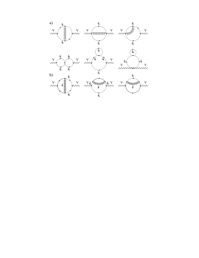
FIG. 3.: Typical Feynman diagrams for the contribution of scalar quarks and gluinos to the $W/Z$–boson self–energies at the two–loop level.

FIG. 4.: Gluon exchange contribution to the $\rho$ parameter at two–loop as a function of $m_{\tilde{q}}$ for the scenarios of Fig. 2.

FIG. 5.: Contribution of the gluino exchange diagrams to $\Delta\rho_{1}^{\rm SUSY}$ for two values of $m_{\tilde{g}}$ in the scenarios of Fig. 2.

REFERENCES

- [1] For reviews see: H.P. Nilles, Phys. Rep. 110, 1 (1984); H.E. Haber and G.L. Kane, Phys. Rep. 117, 75 (1985).
- [2] J. Ellis, hep-ph/9611254; S. Dawson, hep-ph/9612229.
- [3] Particle Data Group, Phys. Rev. D54, 1 (1996).
- [4] S. Bertolini et al., Nucl. Phys. B353, 591 (1991); R. Barbieri and G. Giudice, Phys. Lett. B309, 86 (1993).
- [5] A. Djouadi, G. Girardi, W. Hollik, F. Renard and C. Verzegnassi, Nucl. Phys. B349, 48 (1991); M. Boulware and D. Finnell, Phys. Rev. D44, 2054 (1991).
- [6] See e.g., W. de Boer et al., hep-ph/9609209.
- [7] R. Barbieri et al., Nucl. Phys. B224, 32 (1983); M. Drees and K. Hagiwara, Phys. Rev. D42, 1709 (1990); P. Chankowski et al., Nucl. Phys. B417, 101 (1994).
- [8] M. Veltman, Nucl. Phys. B123, 89 (1977).
- [9] A. Djouadi et al., in preparation.
- [10] A. Djouadi and C. Verzegnassi, Phys. Lett. B195, 265 (1987); A. Djouadi, Nuovo Cim. A100, 357 (1988).
- [11] The three–loop result is also available: K. Chetyrkin, J. Kühn and M. Steinhauser, Phys. Rev. Lett. 75, 3394 (1995); L. Avdeev et al., Phys. Lett. B336, 560 (1994).
- [12] J. Ellis and S. Rudaz, Phys. Lett. B128, 248 (1983).
- [13] We have calculated these contributions in the dimensional regularization scheme. The results should be the same in the dimensional reduction scheme if the electroweak couplings are shifted appropriately, see S.P. Martin and M.T. Vaughn, Phys. Lett. B318, 331 (1993). This will be discussed in detail in Ref. [9].
- [14] G. Degrassi, S. Fanchiotti, P. Gambino, in preparation.
- [15] J. Küblbeck, M. Böhm and A. Denner, Comput. Phys. Commun. 60, 165 (1990).
- [16] G. Weiglein, R. Scharf and M. Böhm, Nucl. Phys. B416, 606 (1994).
- [17] H. Eberl, A. Bartl and W. Majerotto, hep–ph/9603206; A. Djouadi, W. Hollik and C. Jünger, hep–ph/9609419; W. Beenakker et al., hep-ph/9610313.
- [18] B. Kniehl, Int. J. Mod. Phys. A10, 443 (1995).