1 Introduction

The principal interest in the studies of $B$ decays in the context of the standard model (SM) [1] lies in that they provide valuable information on the weak rotation matrix - the Cabibbo-Kobayashi-Maskawa (CKM) matrix [2, 3]. In fact, $B$ decays determine five of the nine CKM matrix elements: $V_{cb},V_{ub},V_{td},V_{ts}$, and $V_{tb}$. The dominant decays of $b$-quark stem from the direct $bcW^{-}$ coupling; then there are decay modes which stem from the CKM-suppressed $buW^{-}$ coupling. These two classes represent the direct charged current (CC) transitions. The electromagnetic penguins and particle-antiparticle mixing(s), representing the so-called flavour changing neutral current processes (FCNC) which have been observed in $B$ decays, are induced as higher order effects (loops) as the SM does not allow direct couplings of the form $bsX$ or $bdX$, where $X=\gamma,Z,H^{0},q\bar{q}$ or a gluon. The effective induced couplings in the SM are governed by the GIM mechanism [4] and are dominated by the intermediate (virtual) top quark contribution - the quark with the largest Yukawa coupling - through the transitions $b\rightarrow tW\rightarrow s$ and $b\rightarrow tW\rightarrow d$. Their quantitative measurements therefore provide information about the properties of the top quark, such as its mass and its weak mixing matrix elements $V_{td},V_{ts}$, and $V_{tb}$.

To extract the CKM matrix elements from the hadronic transitions, one needs to implement the QCD perturbative corrections and calculate the hadronic decay form factors and decay functions for the inclusive and exclusive decays, respectively. A lot of work has gone into calculating the perturbative QCD corrections in $B$ decays and this will be discussed in some detail here. The aspects having to do with non-perturbative physics are not yet under quantitative control, though important advances have been made and partial answers are available. In principle, non-perturbative aspects in $B$ decays can all be calculated in the Lattice-QCD framework. In practice, the impact of this technique is limited due to the inadequacy of the present computer technology which restricts direct computation of the $B$ decay properties involving the $b$-quark with a typical mass of $O(5~{}\mbox{GeV})$. However, useful information on some form factors and coupling constants has been obtained by simulation of the charmed hadron systems and extrapolating to the $b$-quark mass, often also using the constraints from the limiting behaviour of QCD in the $m_{Q}\rightarrow\infty$ limit. There exist other non-perturbative theoretical tools such as the heavy quark effective theory HQET, the QCD sum rules, and the good old potential models, which have been put to good use in the quantitative analyses of experimental results in $B$ decays. We shall review here some representative applications of each of these methods. They, in particular the HQET techniques, have enabled us to determine the two mentioned matrix elements $V_{cb}$ and $V_{ub}$.

The CKM matrix elements $V_{ti};~{}i=d,s,b$ are, in principle, also measurable in the production and decays of the top quark [5]. We note that first measurements of $|V_{tb}|$ have been reported by the CDF collaboration [6], through the ratio $R_{tb}$,

$$R_{tb}\equiv\frac{{\cal B}(t\rightarrow bW)}{\sum_{q=d,s,b}{\cal B}(t\rightarrow qW)}=0.94\pm 0.27(\mbox{stat})\pm 0.13(\mbox{syst})~{}.$$ (1)

Assuming three generations, this yields

$$|V_{tb}|=0.97\pm 0.15\pm 0.07~{},$$ (2)

which is consistent with unity but within experimental errors also consistent with a value which is considerably less than unity, namely at $95\%$ C.L. one gets $|V_{tb}|>0.58$. This measurement is expected to improve significantly in future. A precision of $\delta|V_{tb}|/|V_{tb}|\simeq 12\%$ is projected at the Fermilab Tevatron with an integrated luminosity of $2(fb)^{-1}$, expected to be collected at the turn of this century [6]. Eventually, $|V_{tb}|$ will be measured in experiments at the linear collider(s) with a precision $\delta|V_{tb}|/|V_{tb}|=O(1-2)\%$ from the anticipated accuracy of $\delta\Gamma(t)/\Gamma(t)\simeq 1\%$ on the top quark decay width [7]. However, it will be difficult in the foreseeable future to get quantitatively useful information on $V_{td}$ and $V_{ts}$ from direct decays of the top quark, both due to the anticipated small branching ratios involving these matrix elements,

$${\cal B}(t\rightarrow sW)=O(10^{-3}),~{}~{}~{}{\cal B}(t\rightarrow dW)=O(10^{-4}),$$ (3)

and, more importantly, due to the (present) low efficiency of tagging light-quark jets. This is somewhat discomforting as the direct determination of the CKM matrix elements in top quark decays and their inferred values from FCNC processes, such as the ones from $B$ decays being discussed in these lectures, would have given very stringent constraints on possible new physics or perhaps would have established its existence. It is likely that the FCNC processes in $B$ (and to a lesser extent in $K$) decays will remain the major source of information on $V_{td}$ and $V_{ts}$. We will discuss the present quantitative determinations of these matrix elements and their possible improved measurements at the forthcoming $B$ facilities, such as the $B$ factories, HERA-B, and the hadron colliders (Tevatron and LHC), using rare $B$ decays, $\Delta M_{d}$ and $\Delta M_{s}$.

The weak interaction phase responsible for CP violation in the SM resides dominantly in the matrix elements $V_{td}$ and $V_{ub}$. This is manifest in the Wolfenstein parameterization [8] of the CKM matrix. Hence $B$ decays and mixings involving one or both of these matrix elements are potentially the most promising means to measure CP violation. Since the information on the CP violating phase is rather sparse, essentially confined at present to the decay $K_{L}\rightarrow\pi\pi$, the CP violating asymmetries in $B$ decays will be very welcome and perhaps decisive input in testing the CKM paradigm for CP violation. We shall give a profile of these CP violating asymmetries in $B$ decays and the underlying CKM unitarity triangle based on fitting the present data [9] and will discuss measurements at future facilities which will go a long way in reducing the present uncertainties in the CKM parameter space. These experiments (and the anticipated theoretical progress) have the possibility of putting the quark flavour physics at a comparable precision level as the present electroweak physics in the post-LEPI era.

This writeup is organized as follows: In section 2, we introduce the CKM matrix and the unitarity triangle(s) using the Wolfenstein parametrization for this matrix. In section 3, we discuss the dominant $B$ decay modes, which determine the bulk quantities such as the semileptonic branching ratio ${\cal B}_{SL}(B)$, the average number of charmed particles per $B$ decay $\langle n_{c}\rangle$, and the individual $B$ hadron lifetimes. The present determination of the matrix elements $|V_{cb}|$ and $|V_{ub}|$ from semileptonic $B$ decays is also discussed in this section, using the HQET methods for the former. In section 4, we take up the discussion of the electromagnetic penguins and rare $B$ decays in the SM and make comparison with data in terms of the branching ratio and the photon energy spectrum. This measurement determines the ratio of the CKM matrix elements $|V_{ts}|/|V_{cb}|$ which we quantify. The CKM-suppressed radiative rare decays $B\rightarrow X_{d}+\gamma$ and the corresponding exclusive decays $B\rightarrow(\rho,\omega)\gamma$ are discussed in section 5. Their role in determining the CKM matrix element $|V_{td}|$ (equivalently the CKM-Wolfenstein parameters $\rho$ and $\eta$) is reviewed. The success of this proposal depends in a crucial way on reliable calculations of the so-called long distance (LD) contributions and we discuss some existing estimates of the same. In this section, we also take up the FCNC semileptonic decay $B\rightarrow X_{s}\ell^{+}\ell^{-}$ in the SM model, discussing first the QCD-improved rates and distributions from the short-distance (SD) contribution, including leading power corrections. A quantitative understanding of these decays requires reliable estimates of the LD and non-perturbative effects which we also discuss. In section 6, we give an update of the CKM matrix and the unitarity triangle (UT), taking into account the present measurements and theoretical estimates in a number of $B$ decays and $|\epsilon|$, the CP violating parameter in the kaon sector. The constraints on the CKM parameters from the present LEP bound on $\Delta M_{s}$ are also analyzed. In section 7 we briefly discuss some representative CP-violating asymmetries in $B$ decays and summarize their expected ranges and correlations in the SM. We conclude with a brief summary in section 8. Some of the topics discussed here have also been reviewed in [10].

2 CKM Matrix and the Unitarity Triangle

We start by discussing the flavour changing transitions in the SM. Since QCD is manifestly flavour-diagonal, the only possibility of FCNC transitions is in the electroweak sector. Writing in terms of the physical boson $(W_{\mu}^{\pm},~{}Z_{\mu}^{0},~{}A_{\mu})$ and fermion fields, it is easy to show that the neutral current part of the standard electroweak model is also manifestly flavour-diagonal. Denoting the quarks and leptons by $f_{i}(i=1...6)$, the neutral current in the SM is given by:

$$J_{\mu}^{NC}=\sum_{i}\bar{f}_{i}\bigg{[}\frac{e}{\sin\theta_{W}\cos\theta_{W}}Z_{\mu}\left({I_{3}}_{L}-Q\sin{{}^{2}}\theta_{W}\right)_{i}+eA_{\mu}Q_{i}\bigg{]}f_{i},$$ (4)

where $(I_{3})_{L}=(1-\gamma_{5})/2(I_{3})$ with $I_{3}=+1/2$ for $u_{i}$ and $\nu_{i}$ and $-1/2$ for $d_{i}$ and charged leptons $\ell_{i}$, and $Q_{i}$ is the electric charge of the fermion $f_{i}$ in units of the electron charge, i.e., $Q_{e}=+1$. The electroweak mixing angle in $J_{\mu}^{NC}$, denoted by $\theta_{W}$, has its origin in the diagonalization of the gauge boson mass matrix, and it has the usual definition $\cos\theta_{W}=g_{2}/\sqrt{g_{1}^{2}+g_{2}^{2}}$, with the electric charge defined as $e\equiv g_{2}\sin\theta_{W}$. Concerning the Higgs Yukawa couplings - a potential source of FCNC transitions in general - it is known that the unitary transformations which diagonalize the quark mass matrix also diagonalize the Higgs Yukawa sector in the SM. This is most easily seen by writing the Yukawa sector of the SM Lagrangian, which after spontaneous symmetry breaking has the form

$${\cal L}_{\mbox{Yukawa}}=-\left[\bar{u}_{iL}M^{u}_{ij}u_{jR}+\bar{d}_{iL}M^{d}_{ij}d_{jR}+\bar{\ell}_{iL}M^{\ell}_{ij}\ell_{jR}\right]\left(1+\frac{H}{v_{0}}\right)+h.c.~{},$$ (5)

where the absence of the neutrino mass matrix is conspicuous and represents the SM choice of treating the neutrino massless (equivalently, the absence of the right-handed neutrinos $v_{iR}$). In the basis where the quark masses are diagonal, this takes the form

$${\cal L}_{\mbox{Yukawa}}=-\sum_{i}m_{i}\bar{f}_{i}f_{i}\left(1+\frac{H}{v_{0}}\right)~{},$$ (6)

where $H$ is the Higgs field and $v_{0}$ is the Higgs vacuum expectation value. This manifest flavour diagonal form of ${\cal L}_{\mbox{Yukawa}}$ in general is not maintained in multi-Higgs models and one has to impose discrete symmetries on the Higgs and fermion fields to forbid FCNC couplings in ${\cal L}_{\mbox{Yukawa}}$, as emphasized by Glashow and Weinberg quite some time ago [11]. The absence of such couplings in the SM owes itself to the choice of a single Higgs doublet.

The charged current $J_{\mu}^{CC}$ in the SM, which couples to the $W^{\pm}$, is

$$J_{\mu}^{CC}=\frac{e}{\sqrt{2}\sin\theta_{W}}\left(\bar{u},\bar{c},\bar{t}\right)_{L}\gamma_{\mu}V_{\mbox{\footnotesize CKM}}\left(\begin{array}[]{c}d\\ s\\ b\end{array}\right)_{L},$$ (7)

where $V_{\mbox{\footnotesize CKM}}\equiv V_{L}^{\rm up}V_{L}^{{\rm down}{\dagger}}$ is a $(3\times 3)$ unitary matrix in flavour space, first written down by Kobayashi and Maskawa in 1973 [3]. The matrices $V_{L}^{\rm up}$ and $V_{L}^{\rm down}$ diagonalize the up-type and down type quark mass matrices, respectively. The matrix $V_{\mbox{\footnotesize CKM}}$ is a generalization of the Cabibbo rotation [2] for the three-quark-flavour $(u,d,s)$ case, invented to keep the universality of weak interactions, which took the form of a $(2\times 2)$ matrix by the inclusion of $c$-quark with the GIM construction [4], and is called the Cabibbo-Kobayashi-Maskawa (CKM) matrix. There are no FCNC transitions in the SM at the tree level by construction. They are induced by higher order CC transitions and the resulting FCNC amplitudes are determined by the masses of the intermediate quarks, i.e. they reflect the flavour dependence of the Higgs Yukawa couplings, weighted with the appropriate CKM prefactors.

The charged current in the SM has a $(V-A)$ structure, hence it violates P and C maximally, conserves the electric charge and the lepton- and baryon-number separately, but otherwise there are no restrictions on it except that $V_{\mbox{\footnotesize CKM}}^{{\dagger}}V_{\mbox{\footnotesize CKM}}=1$. In general, ${\cal L}^{CC}$ violates CP due to the possibility of a non-trivial phase in $V_{\mbox{\footnotesize CKM}}$.
Symbolically the matrix $V_{\mbox{\footnotesize CKM}}$ can be written as:

$$V_{\mbox{\footnotesize CKM}}\equiv\left(\begin{array}[]{lll}V_{ud}&V_{us}&V_{ub}\\ V_{cd}&V_{cs}&V_{cb}\\ V_{td}&V_{ts}&V_{tb}\end{array}\right).$$ (8)

For quantitative discussions we need a parametrization of the CKM matrix. The original parametrization due to Kobayashi and Maskawa [3] was constructed from the rotation matrices in the flavour space involving the angles $\theta_{i}~{}(i=1,2,3)$ and a phase $\delta$,

$$V_{\mbox{\footnotesize KM}}=R_{23}(\theta_{3},\delta)R_{12}(\theta_{1},0)R_{23}(\theta_{2},0),$$ (9)

where $0\leq\theta_{i}\leq\pi/2,\,\,0\leq\delta\leq 2\pi$, and $R_{ij}(\theta,\phi)$ denotes a unitary rotation in the $(i,j)$ plane by the angle $\theta$ and the phase $\phi$. The resulting representation is:

$$V_{\mbox{\footnotesize KM}}=\left(\begin{array}[]{lll}c_{1}&-s_{1}c_{3}&-s_{1}s_{3}\\ s_{1}c_{2}&c_{1}c_{2}c_{3}-s_{2}s_{3}e^{i\delta}&c_{1}c_{2}s_{3}+s_{2}c_{3}e^{i\delta}\\ s_{1}s_{2}&c_{1}s_{2}c_{3}+c_{2}s_{3}e^{i\delta}&c_{1}s_{2}s_{3}-c_{2}c_{3}e^{i\delta}\end{array}\right),$$ (10)

with $c_{i}=\cos\theta_{i},s_{i}=\sin\theta_{i}$. This reduces to the usual Cabibbo form for $\theta_{2}=\theta_{3}=0$, with the angle $\theta_{1}$, identified (up to a sign) with the Cabibbo angle. In the PDG review [12], however, another parametrization is advocated which differs from $V_{\mbox{\footnotesize KM}}$ in assigning the complex phases (dominantly) to the (1,3) and (3,1) matrix elements of $V_{\mbox{\footnotesize CKM}}$. An approximate but very useful form of the matrix $V_{\mbox{\footnotesize CKM}}$ is due to Wolfenstein [8]:

$$V_{\mbox{\footnotesize Wolfenstein}}=\left(\begin{array}[]{lll}1-\frac{1}{2}\lambda^{2}&\lambda&A\lambda^{3}(\rho-i\eta)\\ -\lambda&1-\frac{1}{2}\lambda^{2}&A\lambda^{2}\\ A\lambda^{3}(1-\rho-i\eta)&-A\lambda^{2}&1\end{array}\right),$$ (11)

with $\lambda\equiv\sin\theta_{c}\simeq 0.221$. Like other representations, $V_{\footnotesize{\mbox{Wolfenstein}}}$ has also three real parameters called $A$, $\lambda$ and $\rho$, and a phase $\eta$. Since we shall be making extensive use of this parametrization, we write some relations involving the matrix elements of interest in this representation:

$$\frac{|V_{ub}|}{|V_{cb}|}=\lambda\sqrt{\rho^{2}+\eta^{2}},~{}~{}~{}\frac{|V_{td}|}{|V_{cb}|}=\lambda\sqrt{(1-\rho)^{2}+\eta^{2}},\\$$

$$\frac{|V_{td}|}{|V_{ub}|}=\sqrt{\frac{(1-\rho)^{2}+\eta^{2}}{\rho^{2}+\eta^{2}}},~{}~{}~{}\frac{|V_{ts}|}{|V_{cb}|}=1~{},$$ (12)

and the dominant phases are:

$$\Im(V_{ub})=\Im(V_{td})=-A\lambda^{3}\eta.$$ (13)

It should be recalled that the Wolfenstein parameterization given in Eq. (11) is an approximation and in certain situations in the future it may become mandatory to specify the matrix by taking into account the dropped terms in $O(\lambda^{4})$ in $V_{\footnotesize{\mbox{Wolfenstein}}}$. For the present experimental and theoretical accuracy, the representation (11) is entirely adequate and we shall restrict ourselves to this form. Further discussions on this point and suggestions on improved treatment to include higher order terms in $\lambda$ can be seen in [13].

2.1 The CKM unitarity triangles

The CKM matrix elements obey unitarity constraints, which state that any pair of rows, or any pair of columns, of the CKM matrix are orthogonal. This leads to six orthogonality conditions which can be depicted as six triangles in the complex plane of the CKM parameter space [14]. The constraint stemming from the orthogonality condition on the first and third row of $V_{\mbox{\footnotesize CKM}}$,

$$V_{ud}V_{td}^{*}+V_{us}V_{ts}^{*}+V_{ub}V_{tb}^{*}=0$$ (14)

has received considerable attention. Since, as discussed in the introduction, present measurements are consistent with $V_{ud}\simeq 1,~{}V_{tb}\simeq 1$ and $V_{ts}^{*}\simeq-V_{cb}$, the unitarity relation (14) simplifies to:

$$V_{ub}+V_{td}^{*}=V_{us}V_{cb},$$ (15)

which can be conveniently depicted as a triangle relation in the complex plane, as shown in Fig. 1. We shall refer to it as the unitarity triangle (UT). Thus, knowing the sides of the UT, the three angles of this triangle $\alpha,\beta$ and $\gamma$ are determined. These angles are all related to the Kobayashi-Maskawa phase $\delta$ (equivalently the phase $\delta_{13}$ in $V_{\mbox{\footnotesize PDG}}$ or the phase $\eta$ in $V_{\mbox{\footnotesize Wolfenstein}}$), and they can, in principle, be independently measured in various CP-violating $B$ decays. Restricting to the Wolfenstein representation in which the dominant phases reside in the $(13)$ and $(31)$ matrix elements, these angles are defined as follows:

$$\sin 2\alpha = \arg\left(\frac{V_{ub}V_{td}}{V_{ub}^{*}V_{td}^{*}}\right)=\frac{2\eta(\eta^{2}+\rho^{2}-\rho)}{(\rho^{2}+\eta^{2})((1-\rho)^{2}+\eta^{2})}~{},$$

$$\sin 2\beta = \arg\left(-\frac{V_{td}}{V_{td}^{*}}\right)=\frac{2\eta(1-\rho)}{(1-\rho)^{2}+\eta^{2}}~{},$$

$$\sin 2\gamma = \arg\left(-\frac{V_{ub}}{V_{ub}^{*}}\right)=\frac{2\eta\rho}{\rho^{2}+\eta^{2}}~{}.$$ (16)

Some estimates of the angles $\alpha,\beta$ and $\gamma$, and hence CP asymmetries in $B$ decays, can be obtained at present by constraining the parameters of the CKM matrix $\rho$ and $\eta$. Conversely, knowing the CP asymmetries, the parameters $\rho$ and $\eta$ of the CKM matrix can be determined.

As already stated, the matrix elements $V_{cb}$ and $V_{ub}$ are known from the CC $B$ decays. With more data and improved theory (in particular for the so-called heavy-to-light transitions $b\rightarrow u\ell\nu_{\ell}$) one would be able to determine these matrix elements rather precisely. The matrix element $V_{td}$ can, in principle, be determined from the rare decays $b\rightarrow d+~{}\gamma$, $b\rightarrow d+~{}l^{+}l^{-}$, $b\rightarrow d+\nu\bar{\nu}$ (and the corresponding exclusive decays), and $B_{d}^{0}$–$B_{d}^{0}$ mixing. The mass difference $\Delta M_{d}$ already provides a first measurement of $|V_{td}|$. This set of measurements, which involves decay rates and mixing frequencies but not CP-violating asymmetries, then provides another way of determining the triangle, namely by measuring its sides. The lengths of these sides in the Wolfenstein approximation are

$$R_{b} \equiv \frac{1}{\lambda}|\frac{V_{ub}}{V_{cb}}|~{},$$

$$R_{t} \equiv \frac{1}{\lambda}|\frac{V_{td}}{V_{cb}}|~{}.$$ (17)

The CP asymmetries in $B$ decays related to the angles $\alpha,\beta$ and $\gamma$ and the sides of the unitarity triangle obey the geometric relations:

$$R_{b} = \frac{\sin\beta}{\sin\alpha}=\frac{\sin(\alpha+\gamma)}{\sin\alpha}=\frac{\sin\beta}{\sin(\alpha+\beta)}~{},$$

$$R_{t} = \frac{\sin\gamma}{\sin\alpha}=\frac{\sin(\alpha+\beta)}{\sin\alpha}=\frac{\sin\gamma}{\sin(\gamma+\beta)}~{}.$$ (18)

By measuring both the sides and the angles, the UT will be overconstrained which is one of the principal goals of the current and forthcoming experiments in $B$ physics. Before leaving this topic, we note that including the $O(\lambda^{5})$ terms in the imaginary part of the CKM matrix, an additional phase emerges in the matrix element combination $\arg(-V_{cs}^{*}V_{cb}/V_{cb}^{*}V_{cd})$. This phase, being equal to $\lambda^{2}\eta$ is bounded from the CKM fits to be less than $0.025$ and hence very small. However, showing that this CP violating phase is indeed small is both a test of the SM and belongs on the agenda of the forthcoming experiments in $B$ decays.

Figure 1: The unitarity triangle. The angles $\alpha$, $\beta$ and $\gamma$ can be measured via CP violation in the $B$ system and the sides from the CC- and FCNC-induced $B$ decays.

Obviously, there exists a large number of different parametrizations of the CKM matrix. However, since the phases of the quark fields are unphysical quantities, the different parametrizations, emerging from specific choices of these phases, must all be equivalent. The parametrization independent quantities are the absolute values of the matrix elements $|V_{ij}|$ (hence also the angles of the unitarity triangles) and the area of the unitarity triangles, which is the same for all six triangles and is an invariant measure of CP violation. This can be expressed as

$$\mbox{area}[\Delta\mbox{(CKM)}]=\frac{1}{2}A\lambda^{6}\eta$$ (19)

for the Wolfenstein parametrizations of $V_{\mbox{\footnotesize CKM}}$. The Jarlskog invariant denoted by the symbol $J$ [15] is twice this area, which in the standard model is typically of $O(10^{-5})$. It is being debated if the intrinsic smallness of $J$ in the standard model is a serious problem in explaining the measured baryon asymmetry of the universe (BAU), whose quantitative measure is the ratio of the baryon number density to entropy density,

$$\Delta_{B}=\frac{\rho(B)}{s},$$ (20)

with $\Delta_{B}=(0.6-1)\times 10^{-10}$ [12]. Relating the Jarlskog constant to $\Delta B$ is a profound problem and a topic of intense theoretical research. It is an interesting question if $B$ decays will lead to some helpful clues towards understanding this connection. Recent studies indicate that baryogenesis in the SM at the electroweak scale is unlikely [16] due to the LEP constraints on the Higgs boson mass. Very probably, the baryon number violation (as well as the lepton number violation) is governed by the physics at the grand unification scale, which has then little direct influence on $B$ decays. Experiments in $B$ physics will, however, provide an answer to the question if additional CP violating phases in the flavour changing sector are present. These experiments, together with the searches of CP violation in the flavour diagonal sector such as the electric dipole moment of the neutron, will determine the effective low energy theory of CP violation.

3 Dominant $B$ Decays in the Standard Model

We now turn to the mainstream $B$ physics and discuss the dominant decay rates which determine the lifetimes of the $B$ hadrons $\tau_{B}$, the semileptonic branching ratios ${\cal B}_{SL}$, and the charm quark multiplicity in $B$ decays $\langle n_{c}\rangle$ - a quantity which has become an important ingredient in understanding the semileptonic branching ratios.

The effective lowest-order weak interaction Hamiltonian can be expressed in terms of $J_{\mu}^{CC}$, introduced earlier,

$${\cal{H}}_{W}=\frac{G_{F}}{2\sqrt{2}}\left(J_{\mu}^{CC}J^{\mu{\dagger}CC}+\mbox{h.c.}\right),$$ (21)

where $G_{F}$ is the Fermi coupling constant. The calculational framework that is used is QCD and we concentrate first on perturbative QCD improvements of the decay rates and distributions in $B$ decays. The leading order (in $\alpha_{s}$) perturbative QCD improvements using ${\cal{H}_{W}}$ have been worked out in semileptonic processes in [17] - [23], which are modeled on the electromagnetic radiative corrections in the decay of the $\mu$-lepton [24]. For the non-leptonic decays, perturbative QCD corrections are calculated in the effective Hamiltonian approach using the renormalization group techniques [25]$-$[28]. The underlying theoretical framework and its numerous applications in weak decays of the $K$ and $B$ mesons have been reviewed in a comprehensive paper by Buchalla, Buras and Lautenbacher [29], to which we refer for details and confine ourselves here to some selected topics.

Apart from these perturbative QCD improvements, resulting in the so-called QCD-improved quark-parton model, one could also improve the quark-parton model itself by including power corrections in $1/m_{Q}$. The method that is used in discussing such corrections is based on the heavy quark limit of QCD which allows one to do a systematic expansion of decay amplitudes in $1/m_{Q}$, where $m_{Q}\gg\Lambda_{QCD}$, and $\Lambda_{QCD}$ is the QCD scale parameter which is typically of $O(200$ MeV) [12]. This technique [30] - [36] has the satisfying feature that the parton model for heavy quark inclusive decays emerges as the leading term in the expansion of the decay amplitudes. These methods can also be applied to calculate the energy-momentum spectra of the decay products except in the end-point region, where the heavy quark expansion breaks down. Here, one has at present little choice other than smearing the (theoretical and experimental) spectra with weight functions to make meaningful comparison or modeling the non-perturbative effects. We shall return to the discussions of these topics later.

3.1 Inclusive semileptonic decay rates of the $B$ hadrons

We start with the assumption that the inclusive decays of $B$ hadrons can be modeled on the QCD-improved quark model decays. More specifically, while calculating rates, we shall be equating the partial and total decay rates of the $B$ hadrons to the corresponding expressions obtained in the parton model, relying on the heavy quark expansion [30] - [36]:

$$\Gamma(B\rightarrow X)=\Gamma(b\rightarrow x)+O(1/m_{b}^{2})~{}.$$ (22)

For $b$ quark semileptonic decays, one has two partonic CC transitions:

$$b \longrightarrow c\ell^{-}\bar{\nu}_{\ell}~{},$$

$$\longrightarrow u\ell^{-}\bar{\nu}_{\ell}~{}.$$

There exists a close analogy between the $b$ quark decays and $\mu$ decay, $\mu^{-}\longrightarrow e^{-}\bar{\nu}_{e}\nu_{\mu}$, with the identification:

$$[b,(c,u),\bar{\nu}_{\ell},\ell^{-}]\leftrightarrow[\mu^{-},e^{-},\bar{\nu}_{e},\nu_{\mu}].$$ (24)

This analogy holds also at the one loop level; $O(\alpha$) QED corrections to $\mu^{-}$ decay and $O(\alpha_{s}$) QCD corrections to $b$ semileptonic decays are related by simply replacing [17, 18, 19]

$$\alpha\longrightarrow\ \frac{1}{3}\alpha_{s}Tr\sum_{i=1}^{8}\lambda_{i}\lambda_{i}=\frac{4}{3}\alpha_{s},$$ (25)

where $\lambda_{i}$ are the Gell-Mann $SU(3)$ matrices, and $\alpha_{s}$ is the lowest order QCD effective coupling constant,

$$\alpha_{s}=\frac{12\pi}{(33-2n_{f})\ln(\frac{m_{b}^{2}}{\Lambda_{\small{\mbox{QCD}}}^{2}})}\;\;,$$ (26)

where $n_{f}$ is the number of effective quarks. The semileptonic decay rates can then be read off the expression for the $O(\alpha$) radiatively corrected $\mu$-decay rate [24]. The rates for $b\longrightarrow(u,c)\ell\nu_{\ell}$ decays, setting $m_{\ell}=m_{\nu_{\ell}}=0$, are given by the expression:

$$\Gamma_{SL}(b\longrightarrow(u,c)\ell\nu_{\ell})=\Gamma_{0}f(r_{i})\left[1-\frac{2}{3}\frac{\alpha_{s}(m_{b}^{2})}{\pi}g(r_{i})\right],$$ (27)

with $\Gamma_{0}$ being the normalization factor in the lowest-order rate

$$\Gamma_{0}=\frac{G_{F}^{2}}{192\pi^{3}}\mid V_{ib}\mid^{2}m_{b}^{5},$$ (28)

$r_{i}=m_{i}/m_{b}~{}(i=u,b)$, and

$$f(r)=1-8r^{2}+8r^{6}-r^{8}-24r^{4}\ln r.$$ (29)

The function $g(r)$ has the normalization $g(0)=\pi^{2}-\frac{25}{4}$, and numerically $g(0.3)\simeq 2.51$, relevant for the $b\rightarrow u$ and $b\rightarrow c$ transitions, respectively [17, 18, 19]. With $\Lambda_{\mbox{\small QCD}}\simeq 200$ MeV and $n_{f}=5$, this gives about $(15)\%$ corrections to the semileptonic decay widths involving $\ell=e,\mu$, reducing $\Gamma_{SL}$ compared to the lowest order result $\Gamma_{SL}^{(0)}=\Gamma_{0}f(r)$. The corresponding decrease in the decay width for the semileptonic decay $b\rightarrow c\tau\nu_{\tau}$ is obtained by an expression very similar to the above one in which the $\tau$-mass effects are included in the phase space and in the QCD corrections.

$$\Gamma(b\rightarrow c\tau\nu_{\tau})=\Gamma_{0}P(x_{c},x_{\tau},0)\left[1+\frac{2\alpha_{s}(\mu)}{3\pi}g(x_{c},x_{\tau},0)\right]$$ (30)

where $P(x_{1},x_{2},x_{3})$ is the well known three-body phase space factor given for arbitrary masses $x_{i}=m_{i}/m_{b}$ in [37]. The function $g(x_{1},x_{2},x_{3})$ has been calculated for arbitrary arguments in [21] in terms of a one-dimensional integral. The functions $P(x_{1},0,0)$ and $g(x_{c},0,0)$ go over to the functions $f(r)$ and $(-)g(r)$, respectively, given above for the massless lepton case. The numerical values for $g(x_{c},x_{\tau},0)$ and $g(x_{c},0,0)$ are tabulated in [38]. For the default value $x_{c}=0.3$, one has $g(x_{c},x_{\tau},0)=-2.08$, yielding about a 12 % decrease in $\Gamma(b\rightarrow c\tau\nu_{\tau})$ compared to $\Gamma_{SL}^{(0)}(b\rightarrow c\tau\nu_{\tau})$ as a result of the leading order QCD corrections [21]. For more modern calculations of the decay rate $\Gamma_{SL}(b\rightarrow c\tau\nu_{\tau})$, see [22].

3.2 Inclusive non-leptonic decay rates of the $B$ hadrons

The dominant CC-induced non-leptonic and semileptonic decays of $B$ hadrons are governed by the effective Lagrangian,

$${\cal L}_{eff}=-4\frac{G_{F}}{\sqrt{2}}V_{ud}^{*}V_{cb}\left[C_{1}(\mu){\cal O}_{1}(\mu)+C_{2}(\mu){\cal O}_{2}(\mu)\right]$$

$$-4\frac{G_{F}}{\sqrt{2}}V_{us}^{*}V_{cb}\left[C_{1}(\mu){\cal O}_{1}^{\prime}(\mu)+C_{2}(\mu){\cal O}_{2}^{\prime}(\mu)\right]$$

$$-4\frac{G_{F}}{\sqrt{2}}V_{cb}\left[\sum_{\ell=e,\mu,\tau}\bar{\ell}_{L}\gamma_{\mu}\nu_{\ell}\bar{c}_{L}\gamma^{\mu}b_{L}\right]+h.c.~{},$$ (31)

and we have just discussed the $O(\alpha_{s})$ renormalization effects to the matrix elements of the semileptonic piece in ${\cal L}_{eff}$. Here ${\cal O}_{1}$ and ${\cal O}_{2}$ are the colour-octet and colour-singlet four-Fermi operators, respectively ($\alpha$ and $\beta$ are colour indices),

$${\cal O}_{1} = (\bar{d}_{\alpha}u_{\beta})_{L}(\bar{c}_{\beta}b_{\alpha})_{L},$$

$${\cal O}_{2} = (\bar{d}_{\alpha}u_{\alpha})_{L}(\bar{c}_{\beta}b_{\beta})_{L},$$ (32)

and $q_{L}=1/2(1-\gamma_{5})$ denotes a left-handed quark field. The operators ${\cal O}_{i}^{\prime}$ are related to the corresponding fields ${\cal O}_{i}$ by the relacement $\bar{d}\rightarrow\bar{s}$. The octet-octet $({\cal O}_{1})$ and singlet-singlet $({\cal O}_{2})$ operators emerge due to a single gluon exchange between the weak current lines (quark fields) and follow from the colour charge matrix $(T^{a}_{ij})$ algebra:

$$T_{ik}^{a}T_{jl}^{a}=-\frac{1}{2N_{c}}\delta_{ik}\delta_{jl}+\frac{1}{2}\delta_{il}\delta_{jk}~{}.$$ (33)

Here, $N_{c}=3$ for QCD. The Wilson coefficients $C_{i}(\mu)$ are calculated at the scale $\mu=m_{W}$ and then scaled down to the scale typical for $B$ decays, $\mu=O(m_{b})$, using the renormalization group equations, which brings to the fore the influence of strong interactions on the dynamics of weak non-leptonic decays. Without QCD corrections, the two Wilson coefficients have the values $C_{1}(m_{W})=0,~{}C_{2}(m_{W})=1$. Since the operators ${\cal O}_{1}$ and ${\cal O}_{2}$ mix under QCD renormalization, it is convenient to introduce the operators ${\cal O}_{\pm}\equiv({\cal O}_{2}\pm{\cal O}_{1})/2$ having the Wilson coefficients $C_{\pm}$ which renormalize multiplicatively [25]. The results are now known to two-loop accuracy [28]:

$$C_{\pm}(\mu)=L_{\pm}(\mu)\left[1+\frac{\alpha_{s}(m_{W})-\alpha_{s}(\mu)}{4\pi}\frac{\gamma_{\pm}^{(0)}}{2\beta_{0}}\bigg{(}\frac{\gamma_{\pm}^{(1)}}{\gamma_{\pm}^{(0)}}-\frac{\beta_{1}}{\beta_{0}}\bigg{)}+\frac{\alpha_{s}(m_{W})}{4\pi}B_{\pm}\right],$$ (34)

where the multiplicative factor in this expression represents the solution of the RG equations in the leading order QCD [25],

$$L_{\pm}(\mu)=\left[\frac{\alpha_{s}(M_{W})}{\alpha_{s}(\mu)}\right]^{d_{\pm}}~{},$$ (35)

and the exponents have the values $d_{+}=\gamma_{+}^{(0)}/(2\beta_{0})$, $d_{-}=\gamma_{-}^{(0)}/(2\beta_{0})$. The quantities $\gamma_{\pm}^{(i)}$ are the coefficients of the anomalous dimensions involving the operators ${\cal O}_{\pm}$ (and ${\cal O}_{\pm}^{\prime}$),

$$\gamma_{\pm}=\gamma_{\pm}^{(0)}\frac{\alpha_{s}}{4\pi}+\gamma_{\pm}^{(1)}(\frac{\alpha_{s}}{4\pi})^{2}+O(\alpha_{s}^{3}),$$ (36)

with

$$\gamma_{+}^{(0)}=4,~{}~{}\gamma_{-}^{(0)}=-8,~{}~{}\gamma_{+}^{(1)}=-7+\frac{4}{9}n_{f},~{}~{}\gamma_{-}^{(1)}=-14-\frac{8}{9}n_{f},$$ (37)

in the naive dimensional regularization (NDR) scheme, i.e., with anticommuting $\gamma_{5}$. The $\beta_{i}$ are the first two coefficients of the QCD $\beta$-function, and they have the values

$$\beta_{0}=11-\frac{2}{3}n_{f},~{}~{}~{}\beta_{1}=102-\frac{38}{3}n_{f}~{}.$$ (38)

Finally, the functions $B_{\pm}$ are the matching conditions obtained by demanding the equality of the matrix elements of the effective Lagrangian calculated at the scale $\mu=m_{W}$ and in the full theory (i.e., SM) up to terms of $O(\alpha_{s}(m_{W}^{2}))$. They have the values:

$$B_{\pm}=\pm B\frac{N_{c}\mp 1}{2N_{c}},$$ (39)

The constant $B$ and the two-loop anomalous dimension $\gamma_{\pm}^{(1)}$ are both regularization-scheme dependent. In the NDR scheme one has $B=11$. Following [28], we define a scheme-independent quantity $R_{\pm}$,

$$R_{\pm}=B_{\pm}+\frac{\gamma_{\pm}^{(0)}}{2\beta_{o}}\bigg{(}\frac{\gamma_{\pm}^{(1)}}{\gamma_{\pm}^{(0)}}-\frac{\beta_{1}}{\beta_{0}}\bigg{)},$$ (40)

in terms of which the Wilson coefficients read

$$C_{\pm}(\mu)=L_{\pm}(\mu)\left[1+\frac{\alpha_{s}(m_{W})-\alpha_{s}(\mu)}{4\pi}R_{\pm}+\frac{\alpha_{s}(\mu)}{4\pi}B_{\pm}\right].$$ (41)

In this form all the scheme-dependence resides in the coefficients $B_{\pm}$ which is to be cancelled by the scheme-dependence of the matrix elements of the corresponding operators.

In addition to the decays $b\rightarrow c+\bar{u}d,~{}b\rightarrow c+\bar{u}s$ and $b\rightarrow c+\ell\nu_{\ell}$, which are described by the effective Lagrangian (3.2), there are other decays involving the CC transitions $b\rightarrow uX$, $b\rightarrow(c,u)+\bar{c}s$ and $b\rightarrow(c,u)+\bar{c}d$, which are not included in this Lagrangian. In a systematic treatment involving QCD renormalization, one has to enlarge the operator basis to include these transitions and the so-called penguin operators. We shall return to a discussion of this part of the Lagrangian later in these lectures as we discuss rare $B$-decays, where the operator basis will be enlarged and the corresponding Wilson coefficients calculated in the leading logarithmic approximation.

We now discuss the semileptonic branching ratio ${\cal B}_{\mbox{\small SL }}$ for the $B$ mesons and to be specific will consider the case $\ell=e,\mu$. This branching ratio is to a large extent free of the CKM matrix element uncertainties but requires a QCD-improved calculation of the inclusive decay rates, $\Gamma_{\mbox{SL }}$, discussed above, and $\Gamma_{\mbox{tot}}$,

$${\cal B}_{\mbox{SL }}\equiv\frac{\Gamma(B\rightarrow Xe\nu_{e})}{\Gamma_{\mbox{tot}}(B)},$$ (42)

with

$$\Gamma_{\mbox{tot}}(B) = \sum_{\ell=e,\mu,\tau}\Gamma(B\rightarrow X\ell\nu_{\ell})+\Gamma(B\rightarrow X_{c}X)+\Gamma(B\rightarrow X_{c\bar{c}}X)$$ (43)

$$+ \Gamma(B\rightarrow X_{u}X)+\Gamma(B)(\mbox{Penguins})~{}.$$

In the spirit of the parton model, we shall equate $\Gamma(B\rightarrow X_{c}X)=\Gamma(b\rightarrow c\bar{u}d)+~{}\Gamma(b\rightarrow c\bar{u}s)$, noting that the so-called $W$-annihilation and $W$-exchange two-body decays are expected to be small in inclusive $B$ decays. This will be quantified later as we discuss the lifetime differences among $B$ hadrons which arise from the matrix elements of the operators representing these contributions. The corrections for the decay widths $\Gamma(b\rightarrow c\bar{u}d)$ and $\Gamma(b\rightarrow c\bar{u}s)$ are identical neglecting $m_{u}$ and $m_{s}$, and so their contributions can be described by similar functions. The resulting next-to-leading order QCD corrected sum can be expressed as:

$$\Gamma(b\rightarrow c\bar{u}d)+\Gamma(b\rightarrow c\bar{u}s) = \Gamma_{0}P(x_{c},0,0)$$ (44)

$$\times \left[2L(\mu)^{2}_{+}+L(\mu)^{2}_{-}+\frac{\alpha_{s}(M_{W})-\alpha_{s}(\mu)}{2\pi}(2L(\mu)^{2}_{+}R_{+}+L(\mu)^{2}_{-}R_{-})\right.$$

$$+ \frac{2\alpha_{s}(\mu)}{3\pi}\left(\frac{3}{4}(L(\mu)_{+}-L(\mu)_{-})^{2}c_{11}(x_{c})+\frac{3}{4}(L(\mu)_{+}+L(\mu)_{-})^{2}c_{22}(x_{c})\right.$$

$$+\left.\left.\frac{1}{2}(L(\mu)^{2}_{+}-L(\mu)^{2}_{-})(c_{12}(x_{c},\mu)-12\ln\frac{\mu}{m_{b}})\right)\right]$$

$$\equiv 3\Gamma_{0}\eta(\mu)J(x_{c},\mu)~{},$$

with $\eta(\mu)$ representing the leading order QCD corrections. The scheme independent $R_{\pm}$ come from the NLO renormalization group evolution and are given by [28]

$$R_{+} = \frac{10863-1278n_{f}+80n_{f}^{2}}{6(33-2n_{f})^{2}},$$

$$R_{-} = -\frac{15021-1530n_{f}+80n_{f}^{2}}{3(33-2n_{f})^{2}}$$ (45)

For $n_{f}=5$, $R_{+}=6473/3174$, $R_{-}=-9371/1587$. Note that the leading dependence of $L(\mu)_{\pm}$ on the renormalization scale $\mu$ is canceled to ${\cal O}(\alpha_{s})$ by the explicit $\mu$-dependence in the $\alpha_{s}$-correction terms. Virtual gluon and Bremsstrahlung corrections to the matrix elements of four fermion operators are contained in the mass dependent functions $c_{ij}(x)$. The analytic expressions for the functions $c_{11}(x),c_{12}(x),c_{22}(x)$ are given in [38] where also their numerical values are tabulated. Lumping together all the perturbative and finite charm quark corrections in a multiplicative factor $\Delta_{c}(m_{b},x_{c},\alpha_{s}(m_{Z}))$, the perturbatively corrected decay width can be expressed as:

$$\Gamma(b\rightarrow c\bar{u}d)+\Gamma(b\rightarrow c\bar{u}s)=3\Gamma_{0}P(x_{c},0,0)\left[1+\Delta_{c}(x_{c},m_{b},\alpha_{s}(m_{Z}))\right].$$ (46)

For the central values of the parameters used here ($m_{b}=4.8$ GeV, $x_{c}=0.3$, $\mu=m_{b}$ and $\alpha_{s}(m_{Z})=0.117$), the QCD corrections lead to an enhancement [38]:

$$\Delta_{c}(m_{b},x_{c},\alpha_{s}(m_{Z}))=0.17.$$ (47)

Out of this, the bulk is contributed by the leading log factor

$$\eta(\mu)-1=\frac{1}{3}\left(2L_{+}^{2}+L_{-}^{2}\right)-1=0.10~{}.$$ (48)

Next, we equate $\Gamma(B\rightarrow X_{c\bar{c}})=\Gamma(b\rightarrow c\bar{c}s)+\Gamma(b\rightarrow c\bar{c}d)$ and discuss the perturbative QCD corrections to the decay width $\Gamma(b\rightarrow c\bar{c}s)$ and $\Gamma(b\rightarrow c\bar{c}d)$. Neglecting $m_{d}$ and $m_{s}$, an assumption which has been found to be valid to a high accuracy in [39], the corrections in the two decay widths are identical and the result can be written in close analogy with the ones for the decay widths $\Gamma(b\rightarrow c\bar{u}s)$ discussed above.

$$\Gamma(b\rightarrow c\bar{c}s)+\Gamma(b\rightarrow c\bar{c}d) = \Gamma_{0}P(x_{c},x_{c},x_{s})$$ (49)

$$\times \left[2L(\mu)^{2}_{+}+L(\mu)^{2}_{-}+\frac{\alpha_{s}(M_{W})-\alpha_{s}(\mu)}{2\pi}(2L(\mu)^{2}_{+}R_{+}+L(\mu)^{2}_{-}R_{-})\right.$$

$$+ \frac{2\alpha_{s}(\mu)}{3\pi}\left(\frac{3}{4}(L(\mu)_{+}-L(\mu)_{-})^{2}k_{11}(x_{c},\mu)+\frac{3}{4}(L_{+}+L_{-})^{2}k_{22}(x_{c})\right.$$

$$+\left.\left.\frac{1}{2}(L^{2}_{+}-L^{2}_{-})(k_{12}(x_{c})-12\ln\frac{\mu}{m_{b}})\right)\right].$$

The functions $k_{ij}(m_{b},x_{c},\alpha_{s}(m_{Z}))$ have been calculated and their numerical values are tabulated in [40]. Again, lumping together all the perturbative and finite charm quark corrections in a multiplicative factor $\Delta_{cc}(m_{b},x_{c},\alpha_{s}(m_{Z}))$, the perturbatively corrected decay width can be expressed as:

$$\Gamma(b\rightarrow c\bar{c}s)=3\Gamma_{0}P(x_{c},x_{c},x_{s})\left[1+\Delta_{cc}(x_{c},m_{b},\alpha_{s}(m_{Z}))\right].$$ (50)

With the values of the parameters used above, the QCD corrections lead to the following enhancement [39, 40]:

$$\Delta_{cc}(m_{b},x_{c},\alpha_{s}(m_{Z}))=0.37.$$ (51)

This is by far the largest correction to the inclusive rates we have discussed so far. Using pole quark masses and the renormalization scale $\mu=m_{b}$, one gets [39]:

$$\frac{\Gamma(b\rightarrow c\bar{c}s)(NLO)}{\Gamma(b\rightarrow c\bar{c}s)(LO)}=1.32\pm 0.07~{}.$$ (52)

The NLO corrections go in the right direction in bringing theoretical estimates closer to the experimental value for the semileptonic branching ratio. However, this will also lead to enhanced charmed quark multiplicity $\langle n_{c}\rangle$ in $B$ decays, as discussed a little later.

The CKM-suppressed and penguin transitions contribute at a smaller rate to $\Gamma_{\mbox{tot}}(B)$. They are of two kinds:

• $\Gamma(B\rightarrow X_{u}+X)$, which is suppressed due to the CKM matrix element $|V_{ub}|$, with the rate depending on $|V_{ub}|^{2}$, and

• $\Gamma(B)(\mbox{Penguin})$: The so-called penguin transitions $b\rightarrow s+X$, where $X=c\bar{c}$ and $X=g$ (QCD penguins), $X=\gamma$ (electromagnetic penguins), $X=\ell^{+}\ell^{-},\nu\bar{\nu}$ (electroweak penguins).

There are also transitions involving $b\rightarrow d+X$, as well as a host of other rare decays, which can all be neglected. The dominant contributions in the SM add up to [10]:

$$\Gamma(B\rightarrow X_{u}+X)+\Gamma(B)(\mbox{Penguins)}\simeq 1.25\times 10^{-2}\Gamma_{0}~{},$$ (53)

and hence not of much consequence for the semileptonic branching ratio or the $B$ hadron lifetime estimates.

3.3 Power corrections in $\Gamma_{SL}(B)$ and $\Gamma_{NL}(B)$

Before we discuss the numerical results for ${\cal B}_{\mbox{\small SL}}$, we include the $O(1/m_{b}^{2})$ power corrections in the inclusive partonic decay widths. They constitute the first non-trivial corrections to the parton model results and have been calculated using the operator product expansion techniques [30]- [35].

In HQET, the $b$-quark field is represented by a four-velocity-dependent field, denoted by $b_{v}(x)$. To first order in $1/m_{b}$, the $b$-quark field in QCD $b(x)$ and the HQET-field $b_{v}(x)$ are related through:

$$b(x)=e^{-im_{b}v.x}\left[1+i\frac{\not\!\!D}{2m_{b}}\right]b_{v}(x)$$ (54)

The QCD Lagrangian for the $b$ quark in HQET in this order is:

$${\cal L}^{\mbox{\small HQET}}=\bar{b}_{v}iv.\not\!\!Db_{v}+\bar{b}_{v}\frac{i(\not\!\!D)^{2}}{2m_{b}}b_{v}-Z_{b}\bar{b}_{v}\frac{gG_{\alpha\beta}\sigma^{\alpha\beta}}{4m_{b}}b_{v}+O\left[\frac{1}{m_{b}^{2}}\right],$$ (55)

where $Z_{b}$ is a renormalization factor, with $Z_{b}(\mu=m_{b})=1$ and $\not\!\!D=D_{\mu}\gamma^{\mu}$, with $D_{\mu}$ being the covariant derivative. The operator $\bar{b}_{v}(i\not\!\!D)^{2}b_{v}/2m_{b}$ is not renormalized due to the symmetries of HQET. (In technical jargon, this is termed as a consequence of the reparametrization invariance of ${\cal L}^{\mbox{\small HQET}}$.) With this Lagrangian, it has been shown in [30] - [31] that in the heavy quark expansion in order $(1/m_{b}^{2})$, the hadronic corrections can be expressed in terms of two matrix elements

$$\langle B^{(*)}|\bar{b}_{v}(iD)^{2}b_{v}|B^{(*)}\rangle=2m_{B^{(*)}}\lambda_{1},$$

$$\langle B^{(*)}|\bar{b}_{v}\frac{g}{2}\sigma_{\mu\nu}F^{\mu\nu}b_{v}|B^{(*)}\rangle=2d_{B^{(*)}}m_{B^{(*)}}\lambda_{2},$$ (56)

where $F^{\mu\nu}$ is the gluonic field strength tensor, and the constants $d_{B^{(*)}}$ have the value 3 and $-1$ for $B$ and $B^{*}$, respectively. The constant $\lambda_{2}$ can be related to the hyperfine splitting in the $B$ mesons, which gives:

$$\lambda_{2}\simeq\frac{1}{4}(m_{B^{*}}^{2}-m_{B}^{2})=0.12~{}\mbox{GeV}^{2}.$$ (57)

The other quantity $\lambda_{1}$ is the average kinetic energy of the $b$ quark inside a $B$ meson and has been estimated in various ways, using the QCD sum rule approach [41], the virial theorem [42], lattice QCD [43] and data [44]. A range

$$\lambda_{1}=-(0.5\pm 0.3)~{}\mbox{GeV}^{2}$$ (58)

is compatible with most estimates. (For a recent compilation of $\lambda_{1}$ estimates, see [43].) Taking into account these corrections, the semileptonic and non-leptonic decay rates of a $B$ meson $B\rightarrow X\ell\nu_{\ell}$ and $B\rightarrow X_{c}X$ can be written as [31, 32]:

$$\Gamma(B\longrightarrow X_{c}\ell\nu_{\ell}) = \Gamma^{(0)}f(r_{c})\bigg{[}\left(1-\frac{2}{3}\frac{\alpha_{s}(m_{b}^{2})}{\pi}g(r_{c})\right)\left(1+\frac{\lambda_{1}}{2m_{b}^{2}}+\frac{3\lambda_{2}}{2m_{b}^{2}}-\frac{6(1-r_{c})^{4}}{f(r_{c})}\frac{\lambda_{2}}{m_{b}^{2}}\right)$$ (59)

$$\mbox{}+O(\alpha_{s}^{2},\frac{\alpha_{s}}{m_{b}^{2}},\frac{1}{m_{b}^{3}})\bigg{]},$$

and

$$\Gamma(B\longrightarrow X_{c}X) = 3\Gamma^{(0)}\bigg{[}\eta(\mu)J(\mu)\left(1+\frac{\lambda_{1}}{2m_{b}^{2}}+\frac{3\lambda_{2}}{2m_{b}^{2}}-\frac{6(1-r_{c})^{4}}{f(r_{c})}\frac{\lambda_{2}}{m_{b}^{2}}\right)$$ (60)

$$\mbox{}-\left(L_{+}(\mu)^{2}-L_{-}(\mu)^{2}\right)\frac{4(1-r_{c})^{3}}{f(r_{c})}\frac{\lambda_{2}}{m_{b}^{2}}+O(\alpha_{s}^{2},\frac{\alpha_{s}}{m_{b}^{2}},\frac{1}{m_{b}^{3}})\bigg{]},$$

where the product $\eta(\mu)J(\mu)$ denotes the NLO corrected result for the partonic decay discussed above in (44), to which Eq. (60) reduces in the limit $\lambda_{1}=\lambda_{2}=0$.

The decay rates depend on the quark masses, which unlike lepton masses, do not appear as poles in the $S$-matrix nor do the quarks exist as asymptotic states. They are parameters of an interacting theory and hence subject to renormalization effects. Consequently, they require a regularization scheme, such as the $\overline{MS}$ scheme, and a scale, where they are normalized, to become well-defined quantities. For example, the quark masses in the so-called $\overline{MS}$ scheme and the pole masses (OS scheme) are related in the leading order [45],

$$\overline{m}_{Q}(m_{Q})=m_{Q}\left[1-4\frac{\alpha_{s}(m_{Q})}{(3\pi)}+...\right]~{}.$$ (61)

In HQET, quark masses can be expressed in terms of the heavy meson masses $m_{M}$ and the parameters $\lambda_{1},~{}\lambda_{2}$ and a quantity called $\bar{\Lambda}$, where

$$m_{M}=m_{Q}+\bar{\Lambda}-\frac{\lambda_{1}+d_{M}\lambda_{2}}{2m_{Q}}+...$$ (62)

This yields

$$m_{b}-m_{c}=m_{B}-m_{D}+\frac{\lambda_{1}+3\lambda_{2}}{2}(\frac{1}{m_{b}}-\frac{1}{m_{c}})+O(\frac{1}{m^{2}}),$$ (63)

and the quark mass differences can then be calculated knowing $\lambda_{1}$ and $\lambda_{2}$, giving $(m_{b}-m_{c})=(3.4\pm 0.03\pm 0.03)$ GeV [46]. This difference, which determines the inclusive rates and shape of the lepton energy spectrum in semileptonic decays, has also been determined from an analysis of the experimental lepton energy spectrum in $B$ decays, yielding $(m_{b}-m_{c})=3.39\pm 0.01$ GeV for the pole masses [44], in excellent agreement with the QCD sum rule based estimates.

3.4 Numerical estimates of ${\cal B}_{SL}(B)$ and $\langle n_{c}\rangle$

The theoretical framework described in the previous section can now be used to predict two important quantities in $B$ decays ${\cal B}_{SL}(B)$ and $\langle n_{c}\rangle$, which have been measured. Concerning ${\cal B}_{SL}(B)$, there is some discrepancy between the two set of experiments performed at the $\Upsilon(4S)$ and at the $Z^{0}$ resonance, although it must be stressed that these experiments measure a different mixture of $B$ hadrons. The present measurements give:

$${\cal B}_{SL}(B) = (10.37\pm\pm 0.30)\%~{}~{}~{}\mbox{at}~{}\Upsilon(4S)~{}\cite[cite]{[\@@bibref{}{Tomasz95}{}{}]},$$

$${\cal B}_{SL}(B) = (11.11\pm 0.23)\%~{}~{}~{}~{}~{}~{}\mbox{at}~{}Z^{0}~{}\cite[cite]{[\@@bibref{}{Perret95}{}{}]},$$

$$\langle n_{c}\rangle = 1.16\pm 0.05~{}~{}~{}\mbox{at}~{}\Upsilon(4S)~{}\cite[cite]{[\@@bibref{}{Tomasz95}{}{}]}\,$$

$$\langle n_{c}\rangle = 1.23\pm 0.07~{}~{}~{}\mbox{at}~{}Z^{0}~{}\cite[cite]{[\@@bibref{}{Calderini96}{}{}]},$$ (64)

where the number for $\langle n_{c}\rangle$ at the $Z^{0}$ is from the ALEPH collaboration. We use the following average in which the error on ${\cal B}_{SL}(B)$ is inflated to bridge the gap in the experimental measurements [50]:

$${\cal B}_{SL}(B) = (10.90\pm\pm 0.46)\%~{}\,$$

$$\langle n_{c}\rangle = 1.18\pm 0.04~{}.$$ (65)

The theoretical predictions for these quantities have been updated by Bagan et al. [39], and more recently by Neubert and Sachrajda [50], using the same theoretical input. We shall use here the numerical results from [50] where the following ranges of parameters have been used:

$$m_{b}(\mbox{pole})=4.8\pm 0.2~{}\mbox{GeV};~{}~{}~{}\alpha_{s}(m_{Z})=0.117\pm 0.004,~{}~{}~{}m_{b}/2<\mu<2m_{b},\\$$

and $0.25\leq m_{c}/m_{b}\leq 0.33$. Here $m_{b}$ is the pole mass defined to one-loop order in perturbation theory. At order $1/m_{b}^{2}$ in the heavy quark expansion, non-perturbative effects are described by the parameter $\lambda_{2}$, as the dependence on the parameter $\lambda_{1}$ cancels out in calculating ${\cal B}_{SL}(B)$ and $\langle n_{c}\rangle$. This analysis leads to the following values using the pole masses (OS scheme)[50]:

$${\cal B}_{SL} = (12.0\pm 1.0)\%~{}~{}(\mbox{for}~{}\mu=m_{b}),~{}~{}(10.9\pm 1.0)\%~{}~{}(\mbox{for}~{}\mu=m_{b}/2)~{},$$

$$\langle n_{c}\rangle = 1.20\mp 0.06~{}~{}~{}~{}~{}(\mbox{for}~{}\mu=m_{b}),~{}~{}~{}1.21\mp 0.06~{}~{}~{}~{}(\mbox{for}~{}\mu=m_{b}/2).$$ (66)

One could also use, following Bagan et al. [39], the $\overline{\mbox{MS}}$ scheme and the results in this scheme are as follows [50]

$${\cal B}_{SL}(\overline{\mbox{MS}}) = (10.9\pm 0.9)\%~{}~{}(\mbox{for}~{}\mu=m_{b}),~{}~{}(10.3\pm 0.9)\%~{}~{}(\mbox{for}~{}\mu=m_{b}/2)~{},$$

$$\langle n_{c}\rangle = 1.25\mp 0.05~{}~{}~{}~{}~{}(\mbox{for}~{}\mu=m_{b}),~{}~{}~{}1.24\mp 0.06~{}~{}~{}~{}(\mbox{for}~{}\mu=m_{b}/2),$$ (67)

The numbers in the $\overline{\mbox{MS}}$ scheme correspond to using the two-loop anomalous dimension matrix in the running of the quark masses and the errors from various sources have been added in quadrature. The estimates (3.4) and (3.4) show that both $\langle n_{c}\rangle$ and ${\cal B}_{SL}$ are scheme-dependent; in addition ${\cal B}_{SL}$ also depends on the scale $\mu$. A comparison of the theoretical estimates in the OS scheme (eqs. (3.4)) and data on $\langle n_{c}\rangle$ and ${\cal B}_{SL}$ is shown in Fig.  2. Given the parametric dependence on the scale $\mu$ and the ratio $m_{c}/m_{b}$, the agreement between theory and experiment is reasonably good. In the $\overline{\mbox{MS}}$ scheme, the semileptonic branching ratio is generally smaller and $\langle n_{c}\rangle$ somewhat higher (the two are anti-correlated).

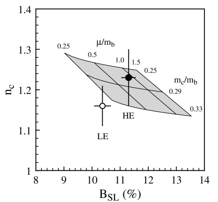
Figure 2: The charm content $n_{c}$ vs. $B_{\small SL}$ in $B$ decays, shown as a function of the quark mass ratio $m_{c}/m_{b}$ and the renormalization scale $\mu/m_{b}$ in the OS scheme. The data show the experimental averages from the $\Upsilon(4S)$ (LE) and $Z^{0}$ (HE) measurements. (Figure taken from [50]).

To make more precise predictions, one has to calculate the missing $O(\alpha_{s}^{2})$ corrections, which, as the experience has it, will considerably reduce the scale dependence. However, equally important is to reduce the present theoretical uncertainty in the ratio $m_{c}/m_{b}$. Here, precise data on the lepton and hadron energy distribution in semileptonic $B$ decays will help. So, while there is certainly much room for improvement, it is fair to conclude that within existing uncertainties the current theoretical estimates for ${\cal B}_{SL}$ and $\langle n_{c}\rangle$ in the SM do not disagree significantly from the corresponding experimental values.

3.5 $B$-Hadron Lifetimes in the Standard Model

A matter closely related to the semileptonic branching ratios is that of the individual $B$ hadron lifetimes. The QCD-improved spectator model gives almost equal lifetimes. Power corrections will split the $B$-baryon lifetime from those of $B_{d}^{0},B^{\pm}$ and $B_{s}$. However, first estimates of these differences are at the few per cent level [31]. The experimental situation has been summarized as of summer 1996 in [51]:

$$\frac{\tau(B^{-})}{\tau(B_{d})}=1.04\pm 0.04;~{}~{}\frac{\tau(B_{s})}{\tau(B_{d})}=0.98\pm 0.05;~{}~{}\frac{\tau(\Lambda_{b})}{\tau(B_{d})}=0.78\pm 0.04~{}.$$ (68)

The subject of exclusive $B$ hadron lifetimes has received renewed theoretical attention lately [50, 52, 54], in which the possibly enhanced roles of the four-Fermion operators involving baryonic states (as compared to the mesonic state) has been studied. We recall that such operators enter at $O(1/m_{b}^{3})$ in the heavy quark expansion discussed above [31]. In this order, there are four such operators, which using the notation of [50], can be expressed as:

$${\cal O}^{q}_{V-A} = (\bar{b}_{L}\gamma_{\mu}q_{L})(\bar{q}_{L}\gamma^{\mu}b_{L}),$$

$${\cal O}^{q}_{S-P} = (\bar{b}_{R}q_{L})(\bar{q}_{L}b_{R}),$$

$${\cal T}^{q}_{V-A} = (\bar{b}_{L}\gamma_{\mu}t_{a}q_{L})(\bar{q}_{L}\gamma^{\mu}t_{a}b_{L}),$$

$${\cal T}^{q}_{S-P} = (\bar{b}_{R}t_{a}q_{L})(\bar{q}_{L}t_{a}b_{R}),$$ (69)

where $t_{a}$ are generators of colour $SU(3)$. The matrix elements of these operators between various $B$-meson and $\Lambda_{b}$-baryons are in general different and this contribution will thus split the decay widths of the various $B$ hadrons. In general, the operators (3.5) introduce eight new parameters corresponding to the matrix elements of these operators. In the large-$N_{c}$ limit, however, it has been argued in [50] that the $B$-mesonic matrix elements of the operators $\langle B_{q}|{\cal O}^{q}_{V-A}|B_{q}\rangle$ and $\langle B_{q}|{\cal O}^{q}_{S-P}|B_{q}\rangle$ are the dominant ones. While accurate numerical estimates require a precise knowledge of these matrix elements, one expects that they give rise typically to the spectator-type effects (using the parton model language):

$$\frac{\Gamma_{\mbox{spec}}}{\Gamma_{\mbox{tot}}}\simeq(\frac{2\pi f_{B}}{m_{B}})^{2}\simeq 5\%~{},$$ (70)

with $f_{B}$ of order 200 MeV. In the case of $\Lambda_{b}$ baryons, one can use the heavy quark spin symmetry to derive two relations involving the operators given above taken between the $\Lambda_{b}$ states. The problem is then reduced to the estimate of two matrix elements which in [50] are taken to be the following:

$$\frac{1}{2m_{\Lambda_{b}}}\langle\Lambda_{b}|{\cal O}^{q}_{V-A}|\Lambda_{b}\rangle\equiv-\frac{f_{B}^{2}m_{B}}{48}r(\frac{\Lambda_{b}}{B_{q}}),$$ (71)

and

$$\langle\Lambda_{b}|\tilde{{\cal O}}^{q}_{V-A}|\Lambda_{b}\rangle=-\tilde{B}\langle\Lambda_{b}|{\cal O}^{q}_{V-A}|\Lambda_{b}\rangle~{},$$ (72)

The operator $\tilde{\cal O}_{V-A}$ is a linear combination of the operators ${\cal T}_{V-A}$ and ${\cal O}_{V-A}$ introduced earlier, $\tilde{{\cal O}}_{V-A}=2{\cal T}_{V-A}+3{\cal O}_{V-A}$, following from colour matrix algebra [50], and $r(\Lambda_{b}/B_{q})$ is the ratio of the squares of the wave functions which can be expressed in terms of the probability of finding a light quark at the location of a $b$ quark inside $\Lambda_{b}$ baryon and the $B$ meson, i.e.

$$r(\frac{\Lambda_{b}}{B_{q}})=\frac{|\Psi^{\Lambda_{b}}_{bq}|^{2}}{|\Psi^{B_{q}}_{b\bar{q}}|^{2}}~{}.$$ (73)

One expects $\tilde{B}=1$ in the valence-quark approximation. However, the ratio $r(\Lambda_{b}/B_{q})$ has a large uncertainty on it, ranging from $r(\Lambda_{b}/B_{q})\simeq 0.5$ in the non-relativistic quark model [53] to $r(\Lambda_{b}/B_{q})=1.8\pm 0.5$ if one uses the ratio of the spin splittings between $\Sigma_{b}$ and $\Sigma_{b}^{*}$ baryons and $B$ and $B^{*}$ mesons, as advocated by Rosner [54] and using the preliminary data from DELPHI, $m(\Sigma_{b}^{*})-m(\Sigma_{b})=(56\pm 16)$ MeV [55].

Using the ball-park estimates that $\tilde{B}$ and $r(\Lambda_{b}/B_{q})$ are both of order unity yields for the lifetime ratio $\tau(\Lambda_{b})/\tau(B_{d})>0.9$ [50], significantly larger than the present world average. Reliable estimates of these constants can be got, in principle, using lattice-QCD and QCD sum rules. Very recently, QCD sum rules have been used to estimate $\langle\Lambda_{b}|\tilde{{\cal O}}^{q}_{V-A}|\Lambda_{b}\rangle$ and $\tilde{B}$, yielding $\langle\Lambda_{b}|\tilde{{\cal O}}^{q}_{V-A}|\Lambda_{b}\rangle=(0.4-1.2)\times 10^{-3}~{}\mbox{GeV}^{3}$ and $\tilde{B}=1.0$ [56]. This corresponds to the parameter $r(\Lambda_{b}/B_{q})$ having a value in the range $r(\Lambda_{b}/B_{q})\simeq 0.1-0.3$, much too small to explain the observed lifetime difference. We mention here the possibility of linear power corrections in the inclusive decay rates, which are not encountered in the explicit power corrections discussed above but may enter via the breakdown of the parton-hadron duality. Phenomenological parametrizations presented in [57] in support of such a scenario are interesting but not persuasive. One must conclude that the lifetime ratio $\tau(\Lambda_{b})/\tau(B_{d})$ remains a puzzle. New and improved measurements are needed, which we trust will be forthcoming from HERA-B and the Tevatron experiments in not-too-distant a future.

Before leaving this section, we mention that from a theoretical point of view one expects measurable lifetime differences between the two mass eigenstates of the $B_{s}^{0}$-$\bar{B_{s}^{0}}$ complex [31]. Recently, leading order perturbative $(O(\Lambda_{\mbox{\small QCD}}/m_{b}))$ and power corrections $(O(m_{s}/m_{b}))$ to the differences in the decay rates $\Gamma_{1}^{s}$ and $\Gamma_{2}^{s}$ of the two mass eigenstates have been analyzed in [58]. The perturbative corrections go along very much the same lines as discussed earlier. Power corrections bring in the four-quark operators already mentioned. Quantitative estimate of $\Delta\Gamma$ requires the knowledge of non-perturbative quantities, bag factors called $B$ and $B_{S}$, involving the expectation values of the operators $\langle{\cal O}^{s}_{V-A}\rangle$ and $\langle{\cal O}^{s}_{S-P}\rangle$, and the pseudoscalar meson coupling constant $f_{B_{s}}$. The resulting expression for the ratio $(\Delta\Gamma/\Gamma)_{B_{s}}$ can be expressed as [58]:

$$\left(\frac{\Delta\Gamma}{\Gamma}\right)_{B_{s}}=\left[aB+bB_{S}+c\right]\left(\frac{f_{B_{s}}}{210~{}\mbox{MeV}}\right)^{2}~{},$$ (74)

where the constants $B$ and $B_{S}$ are the mentioned bag factors and the coefficients $a,b$ and $c$ depend on the parameters such as $m_{b}$ and $\mu$; $c$ incorporates the explicit $1/m_{b}$ corrections. For the choice $B=B_{S}=1$ (corresponding to the vacuum insertion approximation), $m_{b}=4.8$ GeV, $\mu=m_{b}$ and $f_{B_{s}}=210$ MeV, one gets $a=0.009,~{}b=0.211,~{}c=-0.065$, yielding [58]:

$$\left(\frac{\Delta\Gamma}{\Gamma}\right)_{B_{s}}=0.155~{}.$$ (75)

This difference is large enough to be measured in the forthcoming experiments. If accurately measured, $\Delta\Gamma_{B_{s}}$ has the potential of providing an alternative estimate of the mass difference in the $B_{s}^{0}$ - $\bar{B_{s}^{0}}$ complex, $\Delta M_{B_{s}}$, as the ratio $\Delta\Gamma_{B_{s}}/\Delta M_{B_{s}}$, as opposed to the mass difference itself, does not depend on $f_{B_{s}}$. However, there is still some dependence in this ratio on the unknown bag constants and the coefficients. The present determination of this ratio is: $\Delta\Gamma_{B_{s}}/\Delta M_{B_{s}}=(5.6\pm 2.6)\times 10^{-3}$ [58], which is in need of substantial improvement if it has to make any impact on the CKM phenomenology. We shall return to the estimates of $\Delta M_{s}$ and a discussion of the related issues later.

3.6 Determination of $|V_{cb}|$ and $|V_{ub}|$

The CKM matrix element $V_{cb}$ can be obtained from semileptonic decays of $B$ mesons. We shall restrict ourselves to the methods based on HQET [59, 60] to calculate the exclusive semileptonic decay rates and use the heavy quark expansion to estimate the inclusive rates. Concerning exclusive decays, we recall that in the heavy quark limit $(m_{b}\rightarrow\infty)$, it has been observed that all hadronic form factors in the semileptonic decays $B\rightarrow(D,D^{*})\ell\nu_{\ell}$ can be expressed in terms of a single function, the Isgur-Wise function [60]. It has been shown that the HQET-based method works best for $B\rightarrow D^{*}l\nu$ decays, since these are unaffected by $1/m_{Q}$ corrections [61, 62, 63]. Using HQET, the differential decay rate in $B\rightarrow D^{*}\ell\nu_{\ell}$ is

$$\frac{d\Gamma(B\rightarrow D^{*}\ell\bar{\nu})}{d\omega} = \frac{G_{F}^{2}}{48\pi^{3}}(m_{B}-m_{D^{*}})^{2}m_{D^{*}}^{3}\eta_{A}^{2}\sqrt{\omega^{2}-1}(\omega+1)^{2}$$

$$~{}~{}~{}~{}~{}~{}~{}~{}~{}~{}~{}~{}~{}~{}\times[1+\frac{4\omega}{\omega+1}\frac{1-2\omega r+r^{2}}{(1-r)^{2}}]|V_{cb}|^{2}\xi^{2}(\omega)~{},$$

where $r=m_{D^{*}}/m_{B}$, $\omega=v\cdot v^{\prime}$ ($v$ and $v^{\prime}$ are the four-velocities of the $B$ and $D^{*}$ meson, respectively), and $\eta_{A}$ is the short-distance correction to the axial vector form factor. In the leading logarithmic approximation, this was calculated by Shifman and Voloshin some time ago – the so-called hybrid anomalous dimension [64]. In the absence of any power corrections, $\xi(\omega=1)=1$. Estimating the size of the $O(1/m_{b}^{2})$ and $O(1/m_{c}^{2})$ corrections to the Isgur-Wise function, $\xi(\omega)$ has generated some lively theoretical debate [65, 46] but it seems that a convergence has now emerged on their magnitude. We take [46]:

$$\xi(1)=1+\delta(1/m^{2})=0.945\pm 0.025~{}.$$ (77)

The quantity $\eta_{A}$, and its counterpart for the vector current matrix element renormalization, $\eta_{V}$, have now been calculated in the complete next-to-leading order by Czarnecki [66], getting

$$\eta_{A} = 0.960\pm 0.007~{},$$

$$\eta_{V} = 1.022\pm 0.004~{}.$$ (78)

The error on ${\cal F}(1)$ is now dominated by the power corrections in $\xi(1)$, yielding [66]:

$${\cal F}(1)=\xi\cdot\eta_{A}=0.907\pm 0.026~{}.$$ (79)

Since the rate is zero at the kinematic point $\omega=1$, one uses data for $\omega>1$ and an extrapolation procedure to determine $\xi(1)|V_{cb}|$. As the range of accessible energies in the decay $B\rightarrow D^{*}\ell\bar{\nu}$ is rather small $(1~{}<\omega<~{}1.5)$, the extrapolation to the symmetry point can be done using a Taylor expansion around $\omega=1$,

$${\cal F}(\omega)={\cal F}(1)\left[1-\hat{\rho}^{2}(\omega-1)+\hat{c}(\omega-1)^{2}+...\right].$$ (80)

The present experimental input from the exclusive semileptonic channels is based on the data from CLEO, ARGUS, ALEPH, DELPHI and OPAL, which is summarized by Gibbons at the Warsaw conference [67]. He obtains

$$|V_{cb}|\cdot{\cal F}(1)=0.0357\pm 0.0020\pm 0.0014~{}.$$ (81)

Using ${\cal F}(1)$ from Eq. (79), gives the following value:

$$|V_{cb}|=0.0393\pm 0.0021~{}(\rm{expt})\pm 0.0015(\rm{curv})\pm 0.0017~{}(\rm{th}),$$ (82)

where the error from the curvature of the Isgur-Wise function has also been indicated. Combining the errors quadratically gives

$$|V_{cb}|=0.0393\pm 0.0028~{}.$$ (83)

A value of $|V_{cb}|$ has also been obtained from the inclusive semileptonic $B$ decays using heavy quark expansion. The inclusive analysis has the advantage of having very small statistical error. However, as discussed previously, there is about $2\sigma$ discrepancy between the semileptonic branching ratios at the $\Upsilon(4S)$ and in $Z^{0}$ decays. Using an averaged value for the semileptonic decay width from these two sets of measurements and inflating the error as before to take into account the disagreement leads to a value [47]:

$$|V_{cb}|=0.0398\pm 0.0008~{}\mbox{ (expt)}\pm 0.004~{}\mbox{ (th)}~{}.$$ (84)

where the theoretical error estimate ($\pm 10\%)$ has been taken from Neubert [46]. For further discussion of these matters we refer to [65, 46]. The agreement in the values of $|V_{cb}|$ obtained from the exclusive and inclusive semileptonic decays is remarkably good. This can be taken as a quantitative check of the notion of quark-hadron duality in semileptonic decays. We shall use the following values for $|V_{cb}|$ and the Wolfenstein parameter $A$ in the CKM fits discussed later:

$$|V_{cb}|=0.0393\pm 0.0028\Longrightarrow~{}A=0.81\pm 0.058~{}.$$ (85)

The knowledge of the CKM matrix element ratio $|V_{ub}/V_{cb}|$ is based on the analysis of the end-point lepton energy spectrum in semileptonic decays $B\rightarrow X_{u}\ell\nu_{\ell}$ and the measurement of the exclusive semileptonic decays $B\rightarrow(\pi,\rho)\ell\nu_{\ell}$ reported by the CLEO collaboration [47]. As noted in [68], the inclusive measurements suffer from a large extrapolation factor from the measured end-point rate to the total branching ratio, which is model dependent. The exclusive measurements allow a discrimination among a number of models [67], all of which were previously allowed from the inclusive decay analysis alone. It is difficult to combine the exclusive and inclusive measurements to get a combined determination of $|V_{ub}|/|V_{cb}|$. However, it has been noted that the disfavoured models in the context of the exclusive decays are also those which introduce a larger theoretical dispersion in the interpretation of the inclusive $B\rightarrow X_{u}\ell\nu_{\ell}$ data. Excluding them from further consideration, measurements in both the inclusive and exclusive modes are compatible with [67]:

$$\left|\frac{V_{ub}}{V_{cb}}\right|=0.08\pm 0.016~{}.$$ (86)

This gives

$$\sqrt{\rho^{2}+\eta^{2}}=0.363\pm 0.073~{}.$$ (87)

We summarize this section by observing that the bulk properties of $B$ decays are largely accounted for in the standard model. On the theoretical front, parton model estimates of the earlier epoch have been replaced by theoretically better founded calculations with controlled errors. In particular, methods based on HQET and heavy quark expansion have led to a quantitative determination of $|V_{cb}|$ at $\pm 7\%$ accuracy, which makes it after $|V_{ud}|$ and $|V_{us}|$, the third best measured CKM matrix element. The matrix element $|V_{ub}|$ has still large uncertainties ($\pm 20\%)$ and there is every need to reduce this, as this error is one of the two handicaps at present in testing the unitarity of the CKM matrix precisely. The quantities ${\cal B}_{SL}$, $\langle n_{c}\rangle$, and the individual $B$-hadron lifetimes are now in reasonable agreement with data. A completely quantitative comparison requires the missing NLL corrections and in the case of lifetime differences better evaluations of the matrix elements of four-quark operators, which we hope will be forthcoming. Finally, we stress that it will be very helpful to measure the semileptonic branching ratios $B_{SL}$ for the $\Lambda_{b}$ baryons. With the lifetimes of the $B$ hadrons now well measured, such a measurement would allow to compare $\Gamma_{SL}(B_{d}),\Gamma_{SL}(B^{\pm})$ and $\Gamma_{SL}(\Lambda_{b})$, to check the pattern of power corrections in semileptonic decays.

4 Electromagnetic Penguins and Rare $B$ Decays in the Standard Model

We now discuss the FCNC transitions SM which in the SM are induced through the exchange of $W^{\pm}$ bosons in loop diagrams. We shall discuss representative examples from several such transitions involving $B$ decays, starting with the decay $B\rightarrow X_{s}+\gamma$, which has been measured by CLEO [69]. This was preceded by the measurement of the exclusive decay $B\rightarrow K^{\star}+\gamma$ [70]:

$${\cal B}(B\rightarrow X_{s}+\gamma) = (2.32\pm 0.57\pm 0.35)\times 10^{-4}~{},$$ (88)

$${\cal B}(B\rightarrow K^{\star}+\gamma) = (4.2\pm 0.8\pm 0.6)\times 10^{-5}~{},$$ (89)

yielding an exclusive-to-inclusive ratio:

$$R_{K^{*}}=\frac{\Gamma(B\rightarrow K^{\star}+\gamma)}{\Gamma(B\rightarrow X_{s}+\gamma)}=(18.1\pm 6.8)\%~{}.$$ (90)

These decay rates test the SM and the models for decay form factors and we shall study them quantitatively.

The leading contribution to $b\rightarrow s+\gamma$ arises at one-loop from the so-called penguin diagrams and the matrix element in the lowest order can be written as:

$${\cal M}(b\rightarrow s~{}+\gamma)=\frac{G_{F}}{\sqrt{2}}\,\frac{e}{2\pi^{2}}\sum_{i}V_{ib}V_{is}^{*}F_{2}(x_{i})\,q^{\mu}\epsilon^{\nu}\bar{s}\sigma_{\mu\nu}(m_{b}R~{}+~{}m_{s}L)b~{},$$ (91)

where $x_{i}=~{}m_{i}^{2}/m_{W}^{2}$, $q_{\mu}$ and $\epsilon_{\mu}$ are, respectively, the photon four-momentum and polarization vector, the sum is over the quarks, $u,~{}c$, and $t$, and $V_{ij}$ are the CKM matrix elements. The (modified) Inami-Lim function $F_{2}(x_{i})$ derived from the (1-loop) penguin diagrams is given by [71]:

$$F_{2}(x)=\frac{x}{24(x-1)^{4}}\ \left[6x(3x-2)\log x-(x-1)(8x^{2}+5x-7)\right],\\$$

where in writing the expression for $F_{2}(x_{i})$ above we have left out a constant from the function derived by Inami and Lim, since on using the unitarity constraint these sum to zero. It is instructive to write the unitarity constraint for the decays $B\rightarrow X_{s}+\gamma$ in full:

$$V_{tb}V_{ts}^{*}+V_{cb}V_{cs}^{*}+V_{ub}V_{us}^{*}=0~{}.$$ (92)

Now, since the last term in this sum is completely negligible compared to the others (by direct experimental measurements), one could set it to zero enabling us to express the one-loop electromagnetic penguin amplitude as follows:

$${\cal M}(b\rightarrow s~{}+\gamma)=\frac{G_{F}}{\sqrt{2}}\,\frac{e}{2\pi^{2}}\,\lambda_{t}\,(F_{2}(x_{t})-F_{2}(x_{c}))\,q^{\mu}\epsilon^{\nu}\bar{s}\sigma_{\mu\nu}(m_{b}R~{}+~{}m_{s}L)b~{}.$$ (93)

The GIM mechanism [4] is manifest in this amplitude and the CKM-matrix element dependence is factorized in $\lambda_{t}\equiv V_{tb}V_{ts}^{*}$. The measurement of the branching ratio for $B\rightarrow X_{s}+\gamma$ can then be readily interpreted in terms of the CKM-matrix element product $\lambda_{t}/|V_{cb}|$ or equivalently $|V_{ts}|/|V_{cb}|$. In the approximation we are using (i.e., setting $\lambda_{u}=0$), this is equivalent to measuring $|V_{cs}|$. For a quantitative determination of $|V_{ts}|/|V_{cb}|$, however, QCD radiative corrections have to be computed and the contribution of the so-called long-distance effects estimated. We proceed to discuss them below.

4.1 The effective Hamiltonian for $B\rightarrow X_{s}\gamma$

The appropriate framework to incorporate QCD corrections is that of an effective theory obtained by integrating out the heavy degrees of freedom, which in the present context are the top quark and $W^{\pm}$ bosons. This effective theory is an expansion in $1/m_{W}^{2}$ and involves a tower of increasing higher dimensional operators built from the quark fields $(u,d,s,c,b)$, photon, gluons and leptons. The presence of the top quark and of the $W^{\pm}$ bosons is reflected through the effective coefficients of these operators which become functions of their masses. The operator basis depends on the underlying theory and in these lectures we shall concentrate on the standard model. The basis that we shall use is restricted to dimension-6 operators and the operators which vanish on using the equations of motion are not included. The effective Hamiltonian ${\cal H}_{eff}$ given below covers not only the decay $b\rightarrow s+\gamma$, in which we are principally interested in this section, but also other processes such as $b\rightarrow s+g$ and $b\rightarrow s+q\bar{q}$.

It is to be expected in general that due to QCD corrections, which induce operator-mixing, additional contributions with different CKM pre-factors have to be included in the amplitudes. Thus, QCD effects alter the CKM-matrix element dependence of the decay rates for both $B\rightarrow X_{s}+\gamma$ and (more importantly) $B\rightarrow X_{d}+\gamma$. However, with the help of the unitarity condition given above, the CKM matrix dependence in the effective Hamiltonian incorporating the QCD corrections for the decays $B\rightarrow X_{s}+\gamma$ factorizes, and one can write this Hamiltonian as :

$${\cal H}_{eff}(b\rightarrow s+\gamma)=-\frac{4G_{F}}{\sqrt{2}}V_{ts}^{*}V_{tb}\sum_{i=1}^{8}C_{i}(\mu){\cal O}_{i}(\mu),$$ (94)

where the operator basis is chosen to be (here $\mu$ and $\nu$ are Lorentz indices and $\alpha$ and $\beta$ are colour indices)

$${\cal O}_{1} = (\bar{s}_{L\alpha}\gamma_{\mu}b_{L\alpha})(\bar{c}_{L\beta}\gamma^{\mu}c_{L\beta}),$$ (95)

$${\cal O}_{2} = (\bar{s}_{L\alpha}\gamma_{\mu}b_{L\beta})(\bar{c}_{L\beta}\gamma^{\mu}c_{L\alpha}),$$ (96)

$${\cal O}_{3} = (\bar{s}_{L\alpha}\gamma_{\mu}b_{L\alpha})\sum_{q=u,d,s,c,b}(\bar{q}_{L\beta}\gamma^{\mu}q_{L\beta}),$$ (97)

$${\cal O}_{4} = (\bar{s}_{L\alpha}\gamma_{\mu}b_{L\beta})\sum_{q=u,d,s,c,b}(\bar{q}_{L\beta}\gamma^{\mu}q_{L\alpha}),$$ (98)

$${\cal O}_{5} = (\bar{s}_{L\alpha}\gamma_{\mu}b_{L\alpha})\sum_{q=u,d,s,c,b}(\bar{q}_{R\beta}\gamma^{\mu}q_{R\beta}),$$ (99)

$${\cal O}_{6} = (\bar{s}_{L\alpha}\gamma_{\mu}b_{L\beta})\sum_{q=u,d,s,c,b}(\bar{q}_{R\beta}\gamma^{\mu}q_{R\alpha}),$$ (100)

$${\cal O}_{7} = \frac{e}{16\pi^{2}}m_{b}(\bar{s}_{L\alpha}\sigma_{\mu\nu}b_{R\alpha})F^{\mu\nu},$$ (101)

$${\cal O}_{7}^{\prime} = \frac{e}{16\pi^{2}}m_{s}(\bar{s}_{R\alpha}\sigma_{\mu\nu}b_{L\alpha})F^{\mu\nu},$$ (102)

$${\cal O}_{8} = \frac{g}{16\pi^{2}}m_{b}(\bar{s}_{L\alpha}T_{\alpha\beta}^{a}\sigma_{\mu\nu}b_{R\beta})G^{a\mu\nu},$$ (103)

$${\cal O}_{8}^{\prime} = \frac{g}{16\pi^{2}}m_{s}(\bar{s}_{R\alpha}T_{\alpha\beta}^{a}\sigma_{\mu\nu}b_{L\beta})G^{a\mu\nu},$$ (104)

where $e$ and $g_{s}$ are the electromagnetic and the strong coupling constants, and $F_{\mu\nu}$ and $G^{A}_{\mu\nu}$ denote the electromagnetic and the gluonic field strength tensors, respectively. We call attention to the explicit mass factors in ${\cal O}_{7}({\cal O}_{7}^{\prime})$ and ${\cal O}_{8}({\cal O}_{8}^{\prime})$, which will undergo renormalization just as the Wilson coefficients. The dominant contributions in the radiative decays $B\rightarrow X_{s}+\gamma$ arise from the operators ${\cal O}_{2}$, ${\cal O}_{7}$ and ${\cal O}_{8}$, whereas the operators ${\cal O}_{3},...,{\cal O}_{6}$ get coefficients through operator mixing only, which numerically are negligible. Historically, the anomalous dimension matrix was calculated in a truncated basis [72] and this basis is still often used for the sake of ease in calculating the real and virtual corrections, though as we discuss below, now the complete anomalous dimension matrix is available [73].

The perturbative QCD corrections to the decay rate $\Gamma(B\rightarrow X_{s}+\gamma)$ have two distinct contributions:

• Corrections to the Wilson coefficients $C_{i}(\mu)$, calculated with the help of the renormalization group equation, whose solution requires the knowledge of the anomalous dimension matrix in a given order in $\alpha_{s}$.

• Corrections to the matrix elements of the operators ${\cal O}_{i}$ entering through the effective Hamiltonian at the scale $\mu=O(m_{b})$.

The anomalous dimension matrix is needed in order to use the renormalization group and sum up large logarithms, i.e., terms like $\alpha_{s}^{n}(m_{W})\log^{m}(m_{b}/M)$, where $M=m_{t}$ or $m_{W}$ and $m\leq n$ (with $n=0,1,2,...)$. Until recently, only the leading logarithmic corrections $(m=n)$ have been calculated systematically in the complete basis given above [73]. Very recently, the next-to-leading order anomalous dimension has also been calculated and reported this summer by Misiak at the Warsaw conference [74].

Next-to-leading order corrections to the matrix elements are now available completely. They are of two kinds:

• QCD Bremsstrahlung corrections $b\rightarrow s\gamma+g$, which are needed both to cancel the infrared divergences in the decay rate for $B\rightarrow X_{s}+\gamma$ and in obtaining a non-trivial QCD contribution to the photon energy spectrum in the inclusive decay $B\rightarrow X_{s}+\gamma$.

• Next-to-leading order virtual corrections to the matrix elements in the decay $b\rightarrow s+\gamma$.

The Bremsstrahlung corrections were calculated in [75] - [77] in the truncated basis and last year also in the complete operator basis [78], which have been checked in [79]. The higher order matching conditions, i.e., $C_{i}(m_{W})$, are known up to the desired accuracy, i.e., up to $O(\alpha_{s}(M_{W})$ terms [80]. The next-to-leading order virtual corrections have been completed by Greub, Hurth and Wyler recently [81]. We discuss the presently available pieces in the SM calculation of ${\cal B}(B\rightarrow X_{s}+\gamma)$ in the NLO accuracy.

We recall that the Wilson coefficients obey the renormalization group equation

$$\left[\mu\frac{\partial}{\partial\mu}+\beta(g)\frac{\partial}{\partial g}\right]C_{i}\left(\frac{M^{2}_{W}}{\mu^{2}},g\right)=\hat{\gamma}_{ji}(g)C_{j}\left(\frac{M^{2}_{W}}{\mu^{2}},g\right).$$ (105)

The QCD beta function $\beta(g)$ has been defined earlier and $\hat{\gamma}(g)$ is the anomalous dimension matrix, which, to leading logarithmic accuracy, is given by

$$\hat{\gamma}(g)=\gamma_{0}\frac{g^{2}}{16\pi^{2}}.$$ (106)

Here $\gamma_{0}$ is a $8\times 8$ matrix given in [73, 82]. The non-zero initial conditions in the SM are given at the scale $M_{W}$ and read [71]

$$C_{2} = 1$$ (107)

$$C_{7}(M_{W}) = -\frac{1}{2}x\left[\frac{2x^{2}/3+5x/12-7/12}{(x-1)^{3}}-\frac{3x^{2}/2-x}{(x-1)^{4}}\ln x\right],$$ (108)

$$C_{8}(M_{W}) = -\frac{1}{2}x\left[\frac{x^{2}/4-5x/4-1/2}{(x-1)^{3}}+\frac{3x/2}{(x-1)^{4}}\ln x\right],$$ (109)

and $x=m^{2}_{t}/M_{W}^{2}$. Also, for subsequent discussion it is useful to define two effective Wilson coefficients $C_{7}^{\mathit{eff}}(\mu)$ and $C_{8}^{\mathit{eff}}(\mu)$ [82]:

$$C_{7}^{\mathit{eff}} \equiv C_{7}-\frac{C_{5}}{3}-C_{6}\quad,$$

$$C_{8}^{\mathit{eff}} \equiv C_{8}+C_{5}\quad.$$ (110)

The numerical values for the Wilson coefficients at $\mu=M_{W}$ (“Matching Conditions”) and at three other scales $\mu=10.0$ GeV, $5.0$ GeV and $10.0$ GeV can, for example, be seen in [10] and will not be given here. In LO, one gets [82]:

$${\cal B}(B\rightarrow X_{s}+\gamma)=(2.8\pm 0.8)\times 10^{-4},$$

reflecting the parametric uncertainties of the underlying framework.

Now, we discuss the explicit $O(\alpha_{s})$ improvement of the decay rate. The real and virtual $O(\alpha_{s})$ corrections to the matrix element for $b\rightarrow s+\gamma$ at the scale $\mu\approx m_{b}$ form a well-defined gauge invariant albeit scheme-dependent set of corrections. This scheme dependence will be cancelled against the one in the anomalous dimension $\gamma^{(1)}$, as discussed in the context of the dominant contributions to the non-leptonic decays of the $B$ hadron earlier. The results presented here correspond to the NDR scheme.

The Bremsstrahlung corrections in $b\rightarrow s\gamma+g$, calculated in [75] - [77] and [78], were aimed at getting a non-trivial photon energy spectrum at the partonic level. In these papers, the virtual corrections to $b\rightarrow s\gamma$ in $O(\alpha_{s})$ were included only partially by taking into account those virtual diagrams which are needed to cancel the infrared singularities (and also the collinear ones in the limit $m_{s}\rightarrow 0$) generated by the Bremsstrahlung diagram. The emphasis was on deriving the photon energy spectrum in $B\rightarrow X_{s}+\gamma$ away from the end-point $x_{\gamma}\rightarrow 1$ and the Sudakov-improved photon energy spectrum in the region $x_{\gamma}\rightarrow 1$. The left-out virtual diagrams, however, do contribute to the overall decay rate in $B\rightarrow X_{s}+\gamma$. Recently, these virtual correction have been evaluated in [81], neglecting the small contributions from the operators $O_{3}$–$O_{6}$. The additional contribution reduces substantially the scale dependence of the leading order (or partial next-to-leading order) decay width $\Gamma(B\rightarrow X_{s}+\gamma)$, which previously was found to be substantial and constituted a good fraction of the theoretical uncertainty in the inclusive decay rate [83, 82, 84, 78].

Concentrating on the dominant operators $O_{2},~{}O_{7}$ and $O_{8}$, the contribution of the next-to-leading order correction to the matrix element part in $b\rightarrow s+\gamma$ can be expressed as follows:

$${\cal M}={\cal M}_{2}+{\cal M}_{7}+{\cal M}_{8}$$ (111)

and the various terms (including appropriate counter term contributions) can be summarized as [81]:

$${\cal M}_{2}=\langle s\gamma|O_{7}|b\rangle_{tree}\,\frac{\alpha_{s}}{4\pi}\,\left(\ell_{2}\log\frac{m_{b}}{\mu}+r_{2}\right)\quad,$$ (112)

with

$$\ell_{2}=\frac{416}{81}.$$ (113)

$$\Re r_{2} = \frac{2}{243}\,\left\{-833+144\pi^{2}z^{3/2}\right.$$ (114)

$$\hskip 8.5359pt+\left[1728-180\pi^{2}-1296\zeta(3)+(1296-324\pi^{2})L+108L^{2}+36L^{3}\right]\,z$$

$$\hskip 8.5359pt+\left[648+72\pi^{2}+(432-216\pi^{2})L+36L^{3}\right]\,z^{2}$$

$$\hskip 8.5359pt\left.+\left[-54-84\pi^{2}+1092L-756L^{2}\right]\,z^{3}\,\right\}$$

$$\Im r_{2} = \frac{16\pi}{81}\,\left\{-5+\left[45-3\pi^{2}+9L+9L^{2}\right]\,z+\left[-3\pi^{2}+9L^{2}\right]\,z^{2}+\left[28-12L\right]\,z^{3}\,\right\}~{}.$$ (115)

Here, $\Re r_{2}$ and $\Im r_{2}$ denote the real and the imaginary part of $r_{2}$, respectively, $z=(m_{c}/m_{b})^{2}$ and $L=\log(z)$.

The real and virtual corrections associated with the operator $O_{7}$, calculated in [75, 76, 78] can be combined into a modified matrix element for $b\rightarrow s\gamma$, in such a way that its square reproduces the result derived in these papers. This modified matrix element ${\cal M}_{7}^{mod}$ reads [81]:

$${\cal M}_{7}^{mod}=\langle s\gamma|O_{7}|b\rangle_{tree}\,\left(1+\frac{\alpha_{s}}{4\pi}\left(\ell_{7}\,\log\frac{m_{b}}{\mu}+r_{7}\right)\right)$$ (116)

with

$$\ell_{7}=\frac{8}{3}\quad,\quad r_{7}=\frac{8}{9}\,(4-\pi^{2})\quad.$$ (117)

Finally, the result for ${\cal M}_{8}$ is [81]:

$${\cal M}_{8}=\langle s\gamma|O_{7}|b\rangle_{tree}\,\frac{\alpha_{s}}{4\pi}\,\left(\ell_{8}\log\frac{m_{b}}{\mu}+r_{8}\right)\quad,$$ (118)

with

$$\ell_{8}=-\frac{32}{9}\quad,\quad r_{8}=-\frac{4}{27}\,\left(-33+2\pi^{2}-6i\pi\right)\quad.$$ (119)

With the results given above, one can write down the amplitude ${\cal M}(b\rightarrow s\gamma)$ by summing the various contributions already mentioned. Since the relevant scale for a $b$ quark decay is expected to be $\mu\sim m_{b}$, the matrix elements of the operators may be expanded around $\mu=m_{b}$ up to order $O(\alpha_{s})$ and the next-to-leading order result can be written as:

$${\cal M}(b\rightarrow s\gamma)=-\frac{4G_{F}\lambda_{t}}{\sqrt{2}}\,D\,\langle s\gamma|O_{7}(m_{b})|b\rangle_{tree}$$ (120)

with

$$D=C_{7}^{\mathit{eff}}(\mu)+\frac{\alpha_{s}(m_{b})}{4\pi}\left(C_{i}^{(0)eff}(\mu)\gamma_{i7}^{(0)eff}\log\frac{m_{b}}{\mu}+C_{i}^{(0)eff}r_{i}\right)\quad,$$ (121)

where the quantities $\gamma_{i7}^{(0)eff}=\ell_{i}+8\,\delta_{i7}$ are the entries of the (effective) leading order anomalous dimension matrix and the quantities $\ell_{i}$ and $r_{i}$ are given for $i=2,7,8$ in eqs. (113,114), (117) and (119), respectively. The first term, $C_{7}^{\mathit{eff}}(\mu)$, on the r.h.s. of Eq. (121) has to be taken up to next-to-leading logarithmic precision in order to get the full next-to-leading logarithmic result, whereas it is sufficient to use the leading logarithmic values of the other Wilson coefficients in Eq. (121).

The decay width $\Gamma^{virt}$ which follows from ${\cal M}(b\rightarrow s\gamma)$ in Eq. (120) reads

$$\Gamma^{virt}=\frac{m_{b,pole}^{5}\,G_{F}^{2}\lambda_{t}^{2}\alpha_{em}}{32\pi^{4}}\,F\,|D|^{2}\quad,$$ (122)

where the terms of $O(\alpha_{s}^{2})$ in $|D|^{2}$ have been discarded. The factor $F$ in Eq. (122) is

$$F=\left(\frac{m_{b}(\mu=m_{b})}{m_{b,pole}}\right)^{2}=1-\frac{8}{3}\,\frac{\alpha_{s}(m_{b})}{\pi}\quad,$$ (123)

and its origin lies in the explicit presence of $m_{b}$ in the operator $O_{7}$. To get the inclusive decay width for $b\rightarrow s\gamma(g)$, also the Bremsstrahlung corrections (except the part already absorbed above) must be added. The contribution of the operators ${\cal O}_{2}$ and ${\cal O}_{7}$ was calculated already in [75]. As pointed out by Buras et al. [82], the explicit logarithms of the form $\alpha_{s}(m_{b})\log(m_{b}/\mu)$ in Eq. (121) are cancelled by the $\mu$-dependence of $C_{7}^{(0)\mathit{eff}}(\mu)$. Therefore, the scale dependence is significantly reduced by including the virtual corrections completely to this order. This is shown in Fig.  3 (solid curves), which yields an error of $\pm 6\%$ on ${\cal B}(B\rightarrow X_{s}+\gamma)$ varying $\mu$ in the range $m_{b}/2\leq\mu\leq 2m_{b}$. We recall that in the LO calculations, this scale dependence was $\pm 20\%$. The CLEO result is shown as dashed lines. The two other curves (dashed-dotted) represent more stringent assumption on the $\mu$-dependence and we refer to [81] for further details.

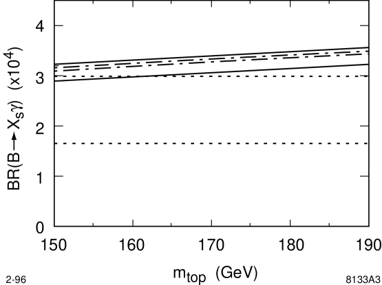
Figure 3: Branching ratio for $b\rightarrow s\gamma(g)$ calculated in [81] with the parameters $|V_{ts}|/|V_{cb}|=1,~{}|V_{tb}|=1,~{}m_{b}^{pole}=4.8$ GeV and $m_{c}/m_{b}=0.29$. The different curves are explained in the text.

4.2 Estimating long-distance effects in $B\rightarrow X_{s}+\gamma$

In order to get the complete amplitude for $B\rightarrow X_{s}+\gamma$ one has to include also the effects of the long-distance contributions, which arise from the matrix elements of the four-quark operators in ${\cal H}_{eff}$, $\langle X_{s}\gamma|{\cal O}_{i}|B\rangle$. It is usual to invoke the hypothesis of factorization, which is then combined with the additional assumption of vector meson dominance, involving the decays $B\rightarrow\sum_{i}V_{i}+X_{s}\rightarrow\gamma+X_{s}$, where $V_{i}=J/\psi,\psi^{\prime},...$ [86] - [89]. One has to ensure that the resulting amplitude ${\cal M}(B\rightarrow X_{s}+\gamma)$ remains manifestly gauge invariant. In practice, this amounts to discarding the longitudinal polarization contribution in the non-leptonic decays $B\rightarrow(J/\psi,\psi^{\prime},...)+X_{s}$, which in fact dominates the decay widths [90], and keeping only the smaller contribution from the transverse polarization of $J/\psi,\psi^{\prime},...$. Following [87, 88], one can write the decay amplitude as:

$${\cal M}(b\rightarrow sJ/\psi)_{T}={G_{F}\over\sqrt{2}}a_{2}V_{cb}V_{cs}^{*}{g_{J/\psi}(m_{J/\psi}^{2})\over m_{b}m_{J/\psi}^{2}}\bar{s}\sigma^{\mu\nu}(1+\gamma_{5})bq_{\nu}\epsilon^{\dagger}_{\mu}(q)\;,$$ (124)

where $g_{\psi}$ is defined as $\langle\psi(q)|\bar{c}\gamma_{\mu}c|0\rangle=-ig_{\psi}(q^{2})\epsilon_{\mu}^{\dagger}(q)$. For the decays under consideration one needs the value of the BSW coefficient $a_{2}$ [91], which has been determined to be $|a_{2}|=0.24\pm 0.04$ [90]. One also needs to evaluate the coupling constant $g_{V}(q^{2})$ at the point $q^{2}=0$. From leptonic decays of vector mesons, one gets, however, $g_{V}(q^{2}=M_{V}^{2})$. As noted in [87, 88], using $g_{V}(q^{2}=0)=g_{V}(q^{2}=M_{V}^{2})$ would substantially overestimate the long-distance contribution due to the expected dynamical suppression of the effective coupling $g_{V}(q^{2})$, as one extrapolates to the point $q^{2}=0$. In fact, such a suppression is supported by HERA data on photoproduction of $J/\psi$. Including all the ($c\bar{c}$) resonances and the short distance contribution ${\cal M}_{SD}$, the two-body decay amplitude ($b\rightarrow s\gamma)$ can be written as

$${\cal M}(b\rightarrow s\gamma)=-{eG_{F}\over 2\sqrt{2}}V_{tb}V_{ts}^{*}[{1\over 4\pi^{2}}m_{b}D(\mu)-a_{2}{2\over 3}\sum_{i}{g_{\psi_{i}}^{2}(0)\over m_{\psi_{i}}^{2}m_{b}}]\bar{s}\sigma^{\mu\nu}(1+\gamma_{5})bF_{\mu\nu}\;,$$ (125)

where $\psi_{i}$ represents the following vector $c\bar{c}$ resonant states: $\psi(1S)$, $\psi(2S)$, $\psi(3770)$, $\psi(4040)$, $\psi(4160)$, and $\psi(4415)$, and $D$ is the function given earlier. Taking this estimate as giving the right order of magnitude for the long-distance contribution, Deshpande et al. [87] conclude that such long-distance effects can be as large as 10%. Other estimates, in particular by Golowich and Pakvasa [88], lead to an even smaller long-distance contribution. Clearly, one can not argue very conclusively if such estimates are completely quantitative due to the assumptions involved. In future, one could improve them by using data from HERA on elastic $J/\psi-$, and $\psi^{\prime}$-photoproduction to get $g_{J/\psi}(0)$ and $g_{\psi^{\prime}}(0)$ directly, reducing at least the extrapolation uncertainties involved in the presently adopted procedure of extracting these coupling constants from the leptonic decay widths of each state and extrapolating to the point $q^{2}=0$ using an Ansatz. In conclusion, LD effects in $B\rightarrow X_{s}+\gamma$ are dynamically suppressed.

4.3 Estimates of ${\cal B}(B\rightarrow X_{s}+\gamma)$ in the Standard Model

In the quantitative estimates of the SM branching ratio ${\cal B}(B\rightarrow X_{s}+\gamma)$ given below we have neglected the LD-contributions. It is theoretically preferable to calculate this quantity in terms of the semileptonic decay branching ratio

$${\cal B}(B\rightarrow X_{s}\gamma)=[\frac{\Gamma(B\rightarrow\gamma+X_{s})}{\Gamma_{SL}}]^{th}\,{\cal B}(B\rightarrow X\ell\nu_{\ell})\qquad,$$ (126)

where, the leading-order QCD corrected $\Gamma_{SL}$ has been given earlier. The leading order power corrections in the heavy quark expansion, discussed in the context of the semileptonic decay rate, are identical in the inclusive decay rates for $B\rightarrow X_{s}+\gamma$ and $B\rightarrow X\ell\nu_{\ell}$, entering in the numerator and denominator in the square bracket, respectively, and hence drop out [30, 31].

The error on the branching ratio ${\cal B}(B\rightarrow X_{s}\gamma)$ comes from the following sources.

1. $\Delta m_{t}$ and $\Delta\mu$: The present value of $m_{t}$ is $m_{t}=175\pm 9$ GeV [6], which is usually interpreted as the pole mass. With this the running top quark mass in the $\overline{MS}$ scheme is $\overline{m_{t}}=166\pm 9$ GeV. This leads to an error of $\pm 4\%$ in ${\cal B}(B\rightarrow X_{s}\gamma)$. The combined error on $\Delta m_{t}$ and $\Delta\mu$ is about $\pm 9\%$ as can be seen in Fig.  3.

2. Errors from the extrinsic parameters ($\Delta(m_{b})$, $\Delta(\alpha_{s}(m_{Z}))$, and $\Delta(BR_{SL})$, the experimental uncertainty on the semileptonic branching ratio): This gives an uncertainty of $\pm 12\%$ on ${\cal B}(B\rightarrow X_{s}+\gamma)$ as estimated in [78], of which half is due to the assumed uncertainty $\Delta(\alpha_{s}(m_{Z}))=0.006$.

As mentioned already, the Wilson coefficient $C_{7}^{\mathit{eff}}$ has been calculated in the next-to-leading order [74]. The NLO corrections are found to be small but the numerical difference is still being worked out. Replacing $C_{7}^{\mathit{eff}}$ by its leading log value yields the branching ratio [10]:

$${\cal B}(B\rightarrow X_{s}+\gamma)=(3.20\pm 0.30\pm 0.38)\times 10^{-4}$$ (127)

where the first error comes from the combined error on $\Delta m_{t}$ and $\Delta\mu$, as can be seen in Fig.  3, and the second from the extrinsic source. Combining the theoretical errors in quadrature gives

$${\cal B}(B\rightarrow X_{s}+\gamma)=(3.20\pm 0.48)\times 10^{-4}.$$ (128)

Using the same input, a branching ratio ${\cal B}(B\rightarrow X_{s}+\gamma)=(3.25\pm 0.50)\times 10^{-4}$ has been calculated in [85]. The error on the NLO branching ratio is now $\pm 15\%$, reduced by a factor 2 from the corresponding LO value. The SM branching ratio ${\cal B}(B\rightarrow X_{s}+\gamma)$ is compatible with the present measurement ${\cal B}(B\rightarrow X_{s}+\gamma)=(2.32\pm 0.67)\times 10^{-4}$ [69]. On its face value, the electroweak penguin rate in the SM is nominally larger than the present experimental value, but due to the large errors this difference is not significant. Nevertheless, this comparison suggests that there is little room for an additive beyond-the-SM contribution, which, for example, is the case in multi-Higgs doublet models. For constraints on such models, see [92]. Expressed in terms of the CKM matrix element ratio, one gets

$$\frac{|V_{ts}|}{|V_{cb}|}=0.85\pm 0.12(\mbox{expt})\pm 0.08(\mbox{th}),$$ (129)

which is within errors consistent with unity, as expected from the unitarity of the CKM matrix.

Finally, we note that the ratio $R_{K^{*}}$ has been calculated in a large number of models. Not surprisingly, taken together they give rise to a large dispersion for this quantity. However, one should stress that QCD sum rules and models based on quark-hadron duality give values which are in good agreement with the CLEO measurements. Some representative results are:

$$R_{K^{*}} = 0.20\pm 0.06~{}~{}[\mbox{Ball}~{}\cite[cite]{[\@@bibref{}{bksnsr}{}{}]}],$$

$$R_{K^{*}} = 0.17\pm 0.05~{}~{}[\mbox{Colangelo et al.}~{}\cite[cite]{[\@@bibref{}{bksnsr}{}{}]}],$$

$$R_{K^{*}} = 0.16\pm 0.05~{}~{}[\mbox{Ali, Braun and Simma}~{}\cite[cite]{[\@@bibref{}{abs93}{}{}]}],$$

$$R_{K^{*}} = 0.16\pm 0.05~{}~{}[\mbox{Narison}~{}\cite[cite]{[\@@bibref{}{bksnsr}{}{}]}],$$

$$R_{K^{*}} = 0.13\pm 0.03~{}~{}[\mbox{Ali \& Greub}~{}\cite[cite]{[\@@bibref{}{ag3}{}{}]}].$$ (130)

4.4 Photon energy spectrum in $B\rightarrow X_{s}+\gamma$

The two-body partonic process $b\rightarrow s\gamma$ yields a photon energy spectrum which is just a discrete line, $1/(\Gamma)d\Gamma(b\rightarrow s\gamma)=\delta(1-x)$, where the scaled photon energy $x$ is defined as $E_{\gamma}=(m_{b}^{2}-m_{s}^{2})/(2\,m_{b})\,x$. The physical photon energy spectrum is built up by convoluting the non-perturbative effects due to the hadronic states involved in the decay and the perturbative QCD corrections, such as $b\rightarrow s\gamma+g$, which give a characteristic Bremsstrahlung spectrum in $x$ in the interval $[0,1]$ peaking near the end-points, $E_{\gamma}\rightarrow E_{\gamma}^{max}$ (or $x\rightarrow 1$) and $E_{\gamma}\rightarrow 0$ (or $x\rightarrow 0$), arising from the soft-gluon and soft-photon configurations, respectively. Near the end-points, one has to improve the spectrum obtained in fixed order perturbation theory. This is usually done in the region $x\rightarrow 1$ by isolating and exponentiating the leading behaviour in $\alpha_{em}\alpha_{s}(\mu)^{m}\log^{2n}(1-x)$ with $m\leq n$, where $\mu$ is a typical momentum in the decay $B\rightarrow X_{s}+\gamma$. The running of $\alpha_{s}$ is a non-leading effect, but as it is characteristic of QCD it modifies the Sudakov-improved end-point photon energy spectrum [95, 96] compared to its analogue in QED [97]. As long as the $s$-quark mass is non-zero, there is no collinear singularity in the spectrum. However, parts of the spectrum have large logarithms of the form $\alpha_{s}\log(m_{b}^{2}/m_{s}^{2})$, which are important near the end-point $x\rightarrow 0$ but their influence persists also in the intermediate photon energy region and they have to be resummed [78, 98]. Implementation of non-perturbative effects is at present model dependent.

We shall confine ourselves to the discussion of the photon energy spectrum calculated in [75, 77, 78], incorporating the perturbatively computed spectrum, discussed in the previous section, and non-perturbative smearing for which a model is used. In this model [19], which admittedly is simplistic but has received some theoretical support in the HQET approach subsequently [32, 100], the $b$ quark in $B$ hadron is assumed to have a Gaussian distributed Fermi motion determined by a non-perturbative parameter, $p_{F}$,

$$\phi(p)=\frac{4}{\sqrt{\pi}{p_{F}}^{3}}\exp(\frac{-p^{2}}{{p_{F}}^{2}})\quad,\quad p=|\vec{p}|$$ (131)

with the wave function normalization $\int_{0}^{\infty}\,dp\,p^{2}\,\phi(p)=1.$ The photon energy spectrum from the decay of the $B$-meson at rest is then given by

$$\frac{d\Gamma}{dE_{\gamma}}=\int_{0}^{p_{max}}\,dp\,p^{2}\,\phi(p)\frac{d\Gamma_{b}}{dE_{\gamma}}(W,p,E_{\gamma})\quad,$$ (132)

where $p_{max}$ is the maximally allowed value of $p$ and $\frac{d\Gamma_{b}}{dE_{\gamma}}$ is the photon energy spectrum from the decay of the $b$-quark in flight, having a momentum-dependent mass $W(p)$. This is calculated in perturbation theory taking into account the appropriate Sudakov behaviour in the $E_{\gamma}$ end-point region at the partonic level.

An analysis of the CLEO photon energy spectrum has been undertaken in [78] to determine the non-perturbative parameters of this model, namely $m_{b}(pole)$ and $p_{F}$. The latter is related to the kinetic energy parameter $\lambda_{1}$ defined earlier in the HQET approach. The experimental errors are still large and the fits result in relatively small $\chi^{2}$ values; the minimum, $\chi^{2}$ is obtained for $p_{F}=450$ MeV and $m_{b}(pole)=4.77$ GeV. While the value of the kinetic energy parameter $\lambda_{1}$ is at present in a state of flux [43] and hence no quantitative conclusions can be drawn, the value of the $b$-quark pole mass determined from the photon energy spectrum is in good agreement with theoretical estimates of the same, namely $m_{b}(pole)=4.8\pm 0.15$ GeV [101, 102]. In Fig. 4 we have plotted the photon energy spectrum normalized to unit area in the interval between 1.95 GeV and 2.95 GeV for the parameters which correspond to the minimum $\chi^{2}$ (solid curve) and for another set of parameters that lies near the $\chi^{2}$-boundary defined by $\chi^{2}=\chi^{2}_{min}+1$. (dashed curve). Data from CLEO [69] are also shown. Further details of this analysis can be seen in [78].

It is a very desirable goal to calculate the photon energy spectrum in $B\rightarrow X_{s}+\gamma$ in a theoretically more robust framework. In this context we note that attempts to calculate the photon and lepton energy spectra in the heavy quark expansion method lead to formal expressions which near the end-point are divergent [32, 99, 100]. Near the end-point, the energy released for the light quark system in the final state is not of $O(m_{b})$ but of the order of the parameter $\bar{\Lambda}=M_{B}-m_{b}\sim O(\Lambda_{\mbox{\small QCD}})$. Thus, the expansion parameter is no longer $1/m_{b}^{2}$ but rather $1/m_{b}\bar{\Lambda}=O(1)$ and the operator product expansion breaks down. This divergent series in the effective theory has to be cleverly resummed and the distributions averaged over momentum bins [103]. The resummation allows us to define, in principle, an effective non-perturbative shape function [103, 96], which though can not be calculated in the effective theory but one could use this concept advantageously to relate the energy spectra in the semileptonic decays $B\rightarrow X_{u}\ell\nu_{\ell}$ and $B\rightarrow X_{s}+\gamma$. Since the perturbative corrections are process-dependent, they have to be included accordingly. This programme remains to be implemented in a phenomenological analysis of data.

Figure 4: Comparison of the normalized photon energy distribution using the CLEO data [69] corrected for detector effects and theoretical distributions from [78] , both normalized to unit area in the photon energy interval between 1.95 GeV and 2.95 GeV. The solid curve corresponds to the values with the minimum $\chi^{2}$, $(m_{q},p_{F})$=(0,  450 MeV), and the dashed curve to the values $(m_{q},p_{F})$=(300 MeV, 310 MeV).

5 Inclusive radiative decays $B\rightarrow X_{d}+\gamma$

The theoretical interest in studying the (CKM-suppressed) inclusive radiative decays $B\rightarrow X_{d}+\gamma$ lies in the first place in the possibility of determining the parameters of the CKM matrix. With that goal in view, one of the interesting quantities in the decays $B\rightarrow X_{d}+\gamma$ is the end-point photon energy spectrum, which has to be measured requiring that the hadronic system $X_{d}$ recoiling against the photon does not contain strange hadrons to separate the large-$E_{\gamma}$ photons from the decay $B\rightarrow X_{s}+\gamma$. Assuming that this is feasible, one can determine from the ratio of the decay rates ${\cal B}(B\rightarrow X_{d}+\gamma)/{\cal B}(B\rightarrow X_{s}+\gamma)$ the CKM-Wolfenstein parameters $\rho$ and $\eta$. This measurement was first proposed in [76], where the photon energy spectra were also worked out.

In close analogy with the $B\rightarrow X_{s}+\gamma$ case discussed earlier, the complete set of dimension-6 operators relevant for the processes $b\rightarrow d\gamma$ and $b\rightarrow d\gamma g$ can be written as:

$${\cal H}_{eff}(b\rightarrow d)=-\frac{4G_{F}}{\sqrt{2}}\,\xi_{t}\,\sum_{j=1}^{8}C_{j}(\mu)\,\hat{O}_{j}(\mu),\quad$$ (133)

where $\xi_{j}=V_{jb}\,V_{jd}^{*}$ with $j=t,c,u$. The operators $\hat{O}_{j},~{}j=1,2$, have implicit in them CKM factors. In the Wolfenstein parametrization [8], one can express these factors as :

$$\xi_{u}=A\,\lambda^{3}\,(\rho-i\eta),~{}~{}~{}\xi_{c}=-A\,\lambda^{3},~{}~{}~{}\xi_{t}=-\xi_{u}-\xi_{c}.$$ (134)

We note that all three CKM-angle-dependent quantities $\xi_{j}$ are of the same order of magnitude, $O(\lambda^{3})$. It is calculationally convenient to define the operators $\hat{O}_{1}$ and $\hat{O}_{2}$ entering in ${\cal H}_{eff}(b\rightarrow d)$ as follows [76]:

$$\hat{O}_{1}=-\frac{\xi_{c}}{\xi_{t}}(\bar{c}_{L\beta}\gamma^{\mu}b_{L\alpha})(\bar{d}_{L\alpha}\gamma_{\mu}c_{L\beta})-\frac{\xi_{u}}{\xi_{t}}(\bar{u}_{L\beta}\gamma^{\mu}b_{L\alpha})(\bar{d}_{L\alpha}\gamma_{\mu}u_{L\beta}),$$

$$\hat{O}_{2}=-\frac{\xi_{c}}{\xi_{t}}(\bar{c}_{L\alpha}\gamma^{\mu}b_{L\alpha})(\bar{d}_{L\beta}\gamma_{\mu}c_{L\beta})-\frac{\xi_{u}}{\xi_{t}}(\bar{u}_{L\alpha}\gamma^{\mu}b_{L\alpha})(\bar{d}_{L\beta}\gamma_{\mu}u_{L\beta}),$$ (135)

with the rest of the operators $\hat{O}_{j}$ defined like their counterparts ${O}_{j}$ in ${\cal H}_{eff}(b\rightarrow s)$, with the obvious replacement $s\rightarrow d$. With this choice, the matching conditions $C_{j}(m_{W})$ and the solutions of the RG equations yielding $C_{j}(\mu)$ become identical for the two operator bases $O_{j}$ and $\hat{O}_{j}$. The essential difference between $\Gamma(B\rightarrow X_{s}+\gamma)$ and $\Gamma(B\rightarrow X_{d}+\gamma)$ lies in the matrix elements of the first two operators $O_{1}$ and $O_{2}$ (in ${\cal H}_{eff}(b\rightarrow s)$) and $\hat{O}_{1}$ and $\hat{O}_{2}$ (in ${\cal H}_{eff}(b\rightarrow d)$). The branching ratio ${\cal B}(B\rightarrow X_{d}+\gamma)$ in the SM can be written as:

$${\cal B}(B\rightarrow X_{d}+\gamma)=D_{1}\lambda^{2}\{(1-\rho)^{2}+\eta^{2}-(1-\rho)D_{2}-\eta D_{3}+D_{4}\},\quad$$ (136)

where the functions $D_{i}$ depend on the parameters $m_{t},m_{b},m_{c},\mu$, as well as the others we discussed in the context of ${\cal B}(B\rightarrow X_{s}+\gamma)$. These functions were first calculated in [76] in the leading logarithmic approximation. Recently, these estimates have been improved in [104], making use of the NLO calculations in [81] discussed in the context of the decay $B\rightarrow X_{s}+\gamma$ earlier. To get the inclusive branching ratio, the CKM parameters $\rho$ and $\eta$ have to be constrained from the unitarity fits. Present data and theory restrict the parameters $\rho$ and $\eta$ to lie in the following range (at 95% C.L.) [9]:

$$0.20 \leq \eta\leq 0.52,$$

$$-0.35 \leq \rho\leq 0.35~{},$$ (137)

which, on using the current lower bound from LEP on the $B_{s}^{0}$ - $\overline{B_{s}^{0}}$ mass difference $\Delta M_{s}>9.2$ (ps)^(-1) [67], restricts $\rho$ to lie in the range $-0.25\leq\rho\leq 0.35$, with $\eta$ not changed significantly. This is based on assuming $\xi_{s}=1.1$, where $\xi_{s}$ is the $SU(3)$-breaking parameter $\xi_{s}=f_{B_{s}}\sqrt{\hat{B}_{B_{s}}}/f_{B_{d}}\sqrt{\hat{B}_{B_{d}}}$. The preferred CKM-fit values are [9]

$$(\rho,\eta)=(0.05,0.36)~{},$$ (138)

for which one gets [104]

$${\cal B}(B\rightarrow X_{d}+\gamma)=1.62\times 10^{-5},$$ (139)

whereas ${\cal B}(B\rightarrow X_{d}+\gamma)=8.0\times 10^{-6}$ and $2.8\times 10^{-5}$ for the other two extremes $\rho=0.35,~{}\eta=0.50$ and $\rho=-\eta=-0.25$, respectively. In conclusion, we note that the functional dependence of ${\cal B}(B\rightarrow X_{d}+\gamma)$ on the Wolfenstein parameters $(\rho,\eta)$ is mathematically different than that of $\Delta M_{s}$. However, since the non-factorizing terms represented by the coefficients $D_{2}$ - $D_{4}$ in the expression for ${\cal B}(B\rightarrow X_{d}+\gamma)$ are numerically small [104], the resulting constraints from this decay mode and $\Delta M_{d}/\Delta M_{s}$ are qualitatively very similar. From the experimental point of view, the situation $\rho<0$ is favourable for both these measurements as in this case one expects (relatively) smaller values for $\Delta M_{s}$ and larger values for the branching ratio ${\cal B}(B\rightarrow X_{d}+\gamma)$, as compared to the $\rho>0$ case which would yield larger $\Delta M_{s}$ and smaller ${\cal B}(B\rightarrow X_{d}+\gamma)$.

5.1 ${\cal B}(B\rightarrow V+\gamma)$ and constraints on the CKM parameters

Exclusive radiative $B$ decays $B\rightarrow V+\gamma$, with $V=K^{*},\rho,\omega$, are also potentially very interesting from the point of view of determining the CKM parameters [93]. The extraction of these parameters would, however, involve a trustworthy estimate of the SD- and LD-contributions in the decay amplitudes.

The SD-contributions in the exclusive decays $(B^{\pm},B^{0})\rightarrow(K^{*\pm},K^{*0})+\gamma$, $(B^{\pm},B^{0})\rightarrow(\rho^{\pm},\rho^{0})+\gamma$, $B^{0}\rightarrow\omega+\gamma$ and the corresponding $B_{s}$ decays, $B_{s}\rightarrow\phi+\gamma$, and $B_{s}\rightarrow K^{*0}+\gamma$, involve the magnetic moment operator ${\cal O}_{7}$ and the related one obtained by the obvious change $s\rightarrow d$, $\hat{O}_{7}$. The transition form factors governing these decays can be generically defined as:

$$\langle V,\lambda|\frac{1}{2}\bar{\psi}\sigma_{\mu\nu}q^{\nu}b|B\rangle=i\epsilon_{\mu\nu\rho\sigma}e^{(\lambda)}_{\nu}p^{\rho}_{B}p^{\sigma}_{V}F_{S}^{B\rightarrow V}(0).$$ (140)

Here $V$ is a vector meson with the polarization vector $e^{(\lambda)}$, $V=\rho,\omega,K^{*}$ or $\phi$; $B$ is a generic $B$-meson $B^{\pm},B^{0}$ or $B_{s}$, and $\psi$ stands for the field of a light $u,d$ or $s$ quark. The vectors $p_{B}$, $p_{V}$ and $q=p_{B}-p_{V}$ correspond to the 4-momenta of the initial $B$-meson and the outgoing vector meson and photon, respectively. Keeping only the SD-contribution leads to obvious relations among the exclusive decay rates, exemplified here by the decay rates for $(B^{\pm},B^{0})\rightarrow(\rho^{\pm},\rho^{0})+\gamma$ and $(B^{\pm},B^{0})\rightarrow(K^{*\pm},K^{*0})+\gamma$:

$$\frac{\Gamma((B^{\pm},B^{0})\rightarrow(\rho^{\pm},\rho^{0})+\gamma)}{\Gamma((B^{\pm},B^{0})\rightarrow(K^{*\pm},K^{*0})+\gamma)}=\frac{|\xi_{t}|^{2}}{|\lambda_{t}|^{2}}\frac{|F_{S}^{B\rightarrow\rho}(0)|^{2}}{|F_{S}^{B\rightarrow K^{*}}(0)|^{2}}\Phi_{u,d}\simeq\kappa_{u,d}\left[\frac{|V_{td}|}{|V_{ts}|}\right]^{2}\,,$$ (141)

where $\Phi_{u,d}$ is a phase-space factor which in all cases is close to 1 and
$\kappa_{i}\equiv[F_{S}^{B_{i}\rightarrow\rho}/F_{S}^{B_{i}\rightarrow K^{*}}]^{2}$. The transition form factors $F_{S}$ are model dependent. Estimates of $F_{S}^{B_{i}\rightarrow K^{*}}$ in the QCD sum rule approach are in good agreement with the CLEO data, as already discussed. The ratios of the form factors, i.e. $\kappa_{i}$, should therefore also be reliably calculable in this approach as they depend essentially only on the SU(3)-breaking effects.

If the SD-amplitudes were the only contributions, the measurements of the CKM-suppressed radiative decays $(B^{\pm},B^{0})\rightarrow(\rho^{\pm},\rho^{0})+\gamma,~{}B^{0}\rightarrow\omega+\gamma$ and $B_{s}\rightarrow K^{*}+\gamma$ could be used in conjunction with the decays $(B^{\pm},B^{0})\rightarrow(K^{*\pm},K^{*0})+\gamma$ to determine the CKM parameters. The present experimental upper limits on the CKM ratio $|V_{td}|/|V_{ts}|$ from radiative $B$ decays are indeed based on this assumption, yielding at 90% C.L.[105]:

$$\left|{V_{td}\over V_{ts}}\right|\leq 0.45-0.56~{},$$ (142)

depending on the models used for the $SU(3)$ breaking effects in the form factors [93, 94].

The possibility of significant LD-contributions in radiative $B$ decays from the light quark intermediate states has been raised in a number of papers [86]. Their amplitudes necessarily involve other CKM matrix elements and hence the simple factorization of the decay rates in terms of the CKM factors involving $|V_{td}|$ and $|V_{ts}|$ no longer holds thereby invalidating the relation (141) given above. As we already discussed, the LD-contributions are small in the exclusive decays $B\rightarrow K^{*}+\gamma$ and so this issue hinges sensitively upon the LD-contributions in the CKM-suppressed decays, $B^{\pm}\rightarrow\rho^{\pm}\gamma$ and $B^{0}\rightarrow(\rho^{0},\omega)\gamma$.

The LD-contributions in $B\rightarrow V+\gamma$, induced by the matrix elements of the four-Fermion operators $\hat{O}_{1}$ and $\hat{O}_{2}$ (likewise $O_{1}$ and $O_{2}$), have been investigated in [106, 107] using a technique [108] which treats the photon emission from the light quarks in a theoretically consistent and model-independent way. This has been combined with the light-cone QCD sum rule approach to calculate both the SD and LD — parity conserving and parity violating — amplitudes in the decays $(B^{\pm},B^{0})\rightarrow(\rho^{\pm},\rho/\omega)+\gamma$. To illustrate this, we concentrate on the $B^{\pm}$ decays $B^{\pm}\rightarrow\rho^{\pm}+\gamma$, and take up the neutral $B$ decays $B^{0}\rightarrow\rho(\omega)+\gamma$ at the end.

The LD-amplitude of the four-Fermion operators $\hat{O}_{1}$, $\hat{O}_{2}$ is dominated by the contribution of the weak annihilation of valence quarks in the $B$ meson and it is color-allowed for the decays of charged $B^{\pm}$ mesons. Using factorization, the LD-amplitude in the decay $B^{\pm}\rightarrow\rho^{\pm}+\gamma$ can be written in terms of the form factors $F_{1}^{L}$ and $F_{2}^{L}$,

$${\cal A}_{long} = -\frac{e\,G_{F}}{\sqrt{2}}V_{ub}V_{ud}^{\ast}\left(C_{2}+\frac{1}{N_{c}}C_{1}\right)m_{\rho}\varepsilon^{(\gamma)}_{\mu}\varepsilon^{(\rho)}_{\nu}$$ (143)

$${}\times\Big{\{}-i\Big{[}g^{\mu\nu}(q\cdot p)-p^{\mu}q^{\nu}\Big{]}\cdot 2F_{1}^{L}(q^{2})+\epsilon^{\mu\nu\alpha\beta}p_{\alpha}q_{\beta}\cdot 2F_{2}^{L}(q^{2})\Big{\}}\,.$$

Estimates from the light-cone QCD sum rules give [107]:

$$F^{L}_{1}/F_{S}=(1.25\pm 0.10)\times 10^{-2}\,,\quad F^{L}_{2}/F_{S}=(1.55\pm 0.10)\times 10^{-2}~{},$$ (144)

where the errors correspond only to the variation of the Borel parameter in the QCD sum rules. Including other possible uncertainties, one expects an accuracy of order 20% for the ratios in (144). The parity-conserving and parity-violating amplitudes turn out to be numerically close to each other in the QCD sum rule approach, $F_{1}^{L}\simeq F^{L}_{2}\equiv F_{L}$, hence the ratio of the LD- and the SD- contributions reduces to a number [107]

$${\cal A}_{long}/{\cal A}_{short}=R_{L/S}^{B^{\pm}\rightarrow\rho^{\pm}\gamma}\cdot\frac{V_{ub}V_{ud}^{\ast}}{V_{tb}V_{td}^{\ast}}~{}.$$ (145)

Using $C_{2}=1.10$, $C_{1}=-0.235$, $C_{7}^{\mathit{eff}}=-0.306$ (corresponding to the scale $\mu=5$ GeV) gives:

$$R_{L/S}^{B^{\pm}\rightarrow\rho^{\pm}\gamma}\equiv\frac{4\pi^{2}m_{\rho}(C_{2}+C_{1}/N_{c})}{m_{b}C_{7}^{\mathit{eff}}}\cdot\frac{F_{L}^{B^{\pm}\rightarrow\rho^{\pm}\gamma}}{F_{S}^{B^{\pm}\rightarrow\rho^{\pm}\gamma}}=-0.30\pm 0.07~{},$$ (146)

which is not small. To get a ball-park estimate of the ratio ${\cal A}_{long}/{\cal A}_{short}$, we take the central value from the CKM fits, $|V_{ub}|/|V_{td}|\simeq 0.33$ [9], yielding

$$|{\cal A}_{long}/{\cal A}_{short}|^{B^{\pm}\rightarrow\rho^{\pm}\gamma}=|R_{L/S}^{B^{\pm}\rightarrow\rho^{\pm}\gamma}|\frac{|V_{ub}V_{ud}|}{|V_{td}V_{tb}|}\simeq 10\%~{}.$$ (147)

Thus, the CKM factors suppress the LD-contributions in ${B^{\pm}\rightarrow\rho^{\pm}\gamma}$.

The analogous LD-contributions in the neutral $B$ decays $B^{0}\rightarrow\rho\gamma$ and $B^{0}\rightarrow\omega\gamma$ are expected to be much smaller, a point that has also been noted in the context of the VMD and quark model based estimates [86]. The corresponding form factors for the decays $B^{0}\rightarrow\rho^{0}(\omega)\gamma$ are obtained from the ones for the decay $B^{\pm}\rightarrow\rho^{\pm}\gamma$ discussed above by the replacement of the light quark charges $e_{u}\rightarrow e_{d}$, which gives the factor $-1/2$; in addition, and more importantly, the LD-contribution to the neutral $B$ decays is colour-suppressed, which reflects itself through the replacement of the BSW-coefficient $a_{1}$ by $a_{2}$ [91]. This yields for the ratio

$$\frac{R_{L/S}^{B^{0}\rightarrow\rho\gamma}}{R_{L/S}^{B^{\pm}\rightarrow\rho^{\pm}\gamma}}=\frac{e_{d}a_{2}}{e_{u}a_{1}}\simeq-0.13\pm 0.05,$$ (148)

where the numbers are based on using $a_{2}/a_{1}=0.27\pm 0.10$ [90]. Thus, in this approach $R_{L/S}^{B^{0}\rightarrow\rho\gamma}\simeq R_{L/S}^{B^{0}\rightarrow\omega\gamma}=0.05$, which in turn gives

$$\frac{{\cal A}_{long}^{B^{0}\rightarrow\rho\gamma}}{{\cal A}_{short}^{B^{0}\rightarrow\rho\gamma}}\leq 0.02.$$ (149)

The above estimate, as well as the one in eq. (147), should be taken only as indicative in view of the approximations made in [106, 107]. That the LD-effects remain small in ${B^{0}\rightarrow\rho\gamma}$ has been supported in a recent analysis based on the soft-scattering of the on-shell hadronic decay products $B^{0}\rightarrow\rho^{0}\rho^{0}\rightarrow\rho\gamma$ [109], though this paper estimates them somewhat higher (between $4-8\%$).

The relations, which follow from the SD-contribution and isospin invariance

$$\Gamma(B^{\pm}\rightarrow\rho^{\pm}\gamma)=2~{}\Gamma(B^{0}\rightarrow\rho^{0}\gamma)=2~{}\Gamma(B^{0}\rightarrow\omega\gamma)~{},$$ (150)

on including the LD-contributions get modified to

$$\frac{\Gamma(B^{\pm}\rightarrow\rho^{\pm}\gamma)}{2\Gamma(B^{0}\rightarrow\rho\gamma)}=\frac{\Gamma(B^{\pm}\rightarrow\rho^{\pm}\gamma)}{2\Gamma(B^{0}\rightarrow\omega\gamma)}=\left|1+R_{L/S}^{B^{\pm}\rightarrow\rho^{\pm}\gamma}\frac{V_{ub}V_{ud}^{\ast}}{V_{tb}V_{td}^{\ast}}\right|^{2}=$$ (151)

$${}=1+2\cdot R_{L/S}V_{ud}\frac{\rho(1-\rho)-\eta^{2}}{(1-\rho)^{2}+\eta^{2}}+(R_{L/S})^{2}V_{ud}^{2}\frac{\rho^{2}+\eta^{2}}{(1-\rho)^{2}+\eta^{2}}\,.$$

where $R_{L/S}\equiv R_{L/S}^{B^{\pm}\rightarrow\rho^{\pm}\gamma}$. The ratio
$\Gamma(B^{\pm}\rightarrow\rho^{\pm}\gamma)/2\Gamma(B^{0}\rightarrow\rho\gamma)(=\Gamma(B^{\pm}\rightarrow\rho^{\pm}\gamma)/2\Gamma(B^{0}\rightarrow\omega\gamma))$, estimated to lie in the range $0.7$ - $1.2$ in [107], constrains the Wolfenstein parameters $(\rho,\eta)$, with the dependence on $\rho$ more marked than on $\eta$.

The ratio of the CKM-suppressed and CKM-allowed decay rates for charged $B$ mesons also gets modified due to the LD contributions. Following [86], we ignore the LD-contributions in $\Gamma(B\rightarrow K^{*}\gamma)$. The ratio of the decay rates in question can therefore be written as:

$$\frac{\Gamma(B^{\pm}\rightarrow\rho^{\pm}\gamma)}{\Gamma(B^{\pm}\rightarrow K^{*\pm}\gamma)}=\kappa_{u}\lambda^{2}[(1-\rho)^{2}+\eta^{2}]$$ (152)

$${}\times\Bigg{\{}1+2\cdot R_{L/S}V_{ud}\frac{\rho(1-\rho)-\eta^{2}}{(1-\rho)^{2}+\eta^{2}}+(R_{L/S})^{2}V_{ud}^{2}\frac{\rho^{2}+\eta^{2}}{(1-\rho)^{2}+\eta^{2}}\Bigg{\}}\,,$$

Using the central value from the estimates $\kappa_{u}=0.59\pm 0.08$ [93], we show the ratio (152) in Fig. 5 as a function of $\rho$ for $\eta=0.2,0.3$, and $0.4$. It is seen that the dependence of this ratio is weak on $\eta$ but it depends on $\rho$ rather sensitively. The effect of the LD-contributions is modest but not negligible, introducing an uncertainty comparable to the $O(15\%)$ uncertainty in the overall normalization due to the $SU(3)$-breaking effects in the quantity $\kappa_{u}$.

Figure 5: Ratio of the CKM-suppressed and CKM-allowed radiative $B$-decay rates
$\Gamma(B^{\pm}\rightarrow\rho^{\pm}\gamma)/\Gamma(B\rightarrow K^{*}\gamma)$ (with $B=B^{\pm}$ or $B^{0}$) as a function of the Wolfenstein parameter $\rho$, a) with $\eta=0.2$ (short-dashed curve), $\eta=0.3$ (solid curve), and $\eta=0.4$ (long-dashed curve). (Figure taken from [107].)

Neutral $B$-meson radiative decays are less-prone to the LD-effects as argued above, and hence one expects that to a good approximation (say, of $O(10\%)$) the ratio of the decay rates for neutral $B$ meson obtained in the approximation of SD-dominance remains valid [93]:

$$\frac{\Gamma(B^{0}\rightarrow\rho^{0}\gamma,\omega\gamma)}{\Gamma(B\rightarrow K^{*}\gamma)}=\kappa_{d}\lambda^{2}[(1-\rho)^{2}+\eta^{2}]~{},$$ (153)

where this relation holds for each of the two decay modes separately.

Finally, combining the estimates for the LD- and SD-form factors in [107] and [93], respectively, and restricting the Wolfenstein parameters in the range $-0.25\leq\rho\leq 0.35$ and $0.2\leq\eta\leq 0.4$ from the CKM-fits [9], one gets the following ranges for the branching ratios:

$${\cal B}(B^{\pm}\rightarrow\rho^{\pm}\gamma) = (1.5\pm 1.1)\times 10^{-6}~{},$$

$${\cal B}(B^{0}\rightarrow\rho\gamma) \simeq {\cal B}(B^{0}\rightarrow\omega\gamma)=(0.65\pm 0.35)\times 10^{-6}~{},$$ (154)

where we have used the experimental value for the branching ratio ${\cal B}(B\rightarrow K^{*}+\gamma)$ [70], adding the errors in quadrature. The large error reflects the poor knowledge of the CKM matrix elements and hence experimental determination of these branching ratios will put rather stringent constraints on the Wolfenstein parameter $\rho$.

In addition to studying the radiative penguin decays of the $B^{\pm}$ and $B^{0}$ mesons discussed above, hadron machines such as HERA-B will be in a position to study the corresponding decays of the $B_{s}^{0}$ meson and $\Lambda_{b}$ baryon, such as $B_{s}^{0}\rightarrow\phi+\gamma$ and $\Lambda_{b}\rightarrow\Lambda+\gamma$, which have not been measured so far. Their estimates can be seen in [110].

5.2 Inclusive decays $B\rightarrow X_{s}\ell^{+}\ell^{-}$ in the SM

The decays $B\rightarrow X_{s}\ell^{+}\ell^{-}$, with $\ell=e,\mu,\tau$, provide a more sensitive search strategy for finding new physics in rare $B$ decays than for example the decay $B\rightarrow X_{s}\gamma$ , which constrains the magnitude of $C_{7}^{\mathit{eff}}$. The sign of $C_{7}^{\mathit{eff}}$, which depends on the underlying physics, is not determined by the measurement of ${\cal B}(B\rightarrow X_{s}+\gamma)$. This sign, which in our convention is negative in the SM, is in general model dependent. It is known (see for example [111]) that in supersymmetric (SUSY) models, both the negative and positive signs are allowed as one scans over the allowed SUSY parameter space. We recall that for low dilepton masses, the differential decay rate for $B\rightarrow X_{s}\ell^{+}\ell^{-}$ is dominated by the contribution of the virtual photon to the charged lepton pair, which in turn depends on the effective Wilson coefficient $C_{7}^{\mathit{eff}}$. However, as is well known, the $B\rightarrow X_{s}\ell^{+}\ell^{-}$  amplitude in the standard model has two additional terms, arising from the two FCNC four-Fermi operators , which are not constrained by the $B\rightarrow X_{s}+\gamma$ data. Calling their coefficients $C_{9}$ and $C_{10}$, it has been argued in [111] that the signs and magnitudes of all three coefficients $C_{7}^{\mathit{eff}}$, $C_{9}$ and $C_{10}$ can, in principle, be determined from the decays $B\rightarrow X_{s}+\gamma$ and $B\rightarrow X_{s}\ell^{+}\ell^{-}$ .

The SM-based rates for the decay $b\rightarrow s\ell^{+}\ell^{-}$ , calculated in the free quark decay approximation, have been known in the LO approximation for some time [72]. The required NLO calculation is in the meanwhile available, which reduces the scheme-dependence of the LO effects in these decays [113]. In addition, long-distance (LD) effects, which are expected to be very important in the decay $B\rightarrow X_{s}\ell^{+}\ell^{-}$ [114], have also been estimated from data on the assumption that they arise dominantly due to the charmonium resonances $J/\psi$ and $\psi^{\prime}$ and higher resonances through the decay chains $B\rightarrow X_{s}J/\psi(\psi^{\prime},...)\rightarrow X_{s}\ell^{+}\ell^{-}$. Likewise, the leading $(1/{m_{b}}^{2})$ power corrections to the partonic decay rate and the dilepton invariant mass distribution have been calculated with the help of the operator product expansion in the effective heavy quark theory [33]. The results of [33] have, however, not been confirmed in a recent calculation [36], which finds that the power corrections in the branching ratio ${\cal B}(B\rightarrow X_{s}\ell^{+}\ell^{-})$ are small. Moreover, the end-point dilepton invariant mass spectrum in this order is not calculable in the heavy quark expansion, which requires either resummation in the context of the HQE approach or a non-perturbative model. We review the salient features of the decay $B\rightarrow X_{s}\ell^{+}\ell^{-}$ here.

The amplitude for $B\rightarrow X_{s}\ell^{+}\ell^{-}$ is calculated in the effective theory approach, which we have discussed earlier, by extending the operator basis of the effective Hamiltonian introduced in Eq. (94):

$${\cal H}_{eff}(b\rightarrow s+\gamma;b\rightarrow s+\ell^{+}\ell^{-})={\cal H}_{eff}(b\rightarrow s+\gamma)-\frac{4G_{F}}{\sqrt{2}}V_{ts}^{*}V_{tb}\left[C_{9}{\cal O}_{9}+C_{10}{\cal O}_{10}\right],$$ (155)

where the two additional operators are:

$${\cal O}_{9} = \frac{\alpha}{4\pi}\bar{s}_{\alpha}\gamma^{\mu}P_{L}b_{\alpha}\bar{\ell}\gamma_{\mu}\ell,$$

$${\cal O}_{10} = \frac{\alpha}{4\pi}\bar{s}_{\alpha}\gamma^{\mu}P_{L}b_{\alpha}\bar{\ell}\gamma_{\mu}\gamma_{5}\ell~{}.$$ (156)

The analytic expressions for $C_{9}(m_{W})$ and $C_{10}(m_{W})$ can be seen in [113] and will not be given here. We recall that the coefficient $C_{9}$ in LO is scheme-dependent. However, this is compensated by an additional scheme-dependent part in the (one loop) matrix element of ${\cal O}_{9}$. We call the sum $C_{9}^{\mathit{eff}}$, which is scheme-independent and enters in the physical decay amplitude given below,

$${\cal M}(b\rightarrow s+\ell^{+}\ell^{-})=\frac{4G_{F}}{\sqrt{2}}V_{ts}^{*}V_{tb}\frac{\alpha}{\pi}$$

$$\times \left[C_{9}^{\mathit{eff}}\bar{s}\gamma^{\mu}P_{L}b\bar{\ell}\gamma_{\mu}\ell+C_{10}\bar{s}\gamma^{\mu}P_{L}b\bar{\ell}\gamma_{\mu}\gamma_{5}\ell-2C_{7}^{\mathit{eff}}\bar{s}i\sigma_{\mu\nu}\frac{q^{\nu}}{q^{2}}(m_{b}P_{R}+m_{s}P_{L})b\bar{\ell}\gamma^{\mu}\ell\right],$$

with

$$C_{9}^{\mathit{eff}}(\hat{s})\equiv C_{9}\eta({\hat{s}})+Y(\hat{s})~{},$$ (158)

where $\hat{s}=q^{2}/m_{b}^{2}$. The function $Y(\hat{s})$ is the one-loop matrix element of ${\cal O}_{9}$ and can be seen in literature [10, 113]. The dilepton invariant mass distribution in $B\rightarrow X_{s}\ell^{+}\ell^{-}$ (ignoring lepton masses) is,

$${{\rm d}{\cal B}(\hat{s})\over{\rm d}\hat{s}} = {\cal B}_{sl}\frac{\alpha^{2}}{4\pi^{2}}\frac{\lambda_{t}^{2}}{|V_{cb}|^{2}}\frac{1}{f(\hat{m}_{c})\kappa(\hat{m}_{c})}u(\hat{s})\left[\vphantom{\frac{1}{1}}\left(|C_{9}^{\mathit{eff}}(\hat{s})|^{2}+C_{10}^{2}\right)\alpha_{1}(\hat{s},\hat{m}_{s})\right.$$ (159)

$$\left.+\frac{4}{\hat{s}}(C^{eff}_{7})^{2}\alpha_{2}(\hat{s},\hat{m}_{s})+12\alpha_{3}(\hat{s},\hat{m}_{s})C^{eff}_{7}{\cal\Re}(C_{9}^{\mathit{eff}}(\hat{s}))\right],$$

with $u(\hat{s})=\sqrt{\left[\hat{s}-(1+\hat{m_{s}})^{2}\right]\left[\hat{s}-(1-\hat{m_{s}})^{2}\right]}$, and $f(\hat{m}_{c})$ has been given earlier; likewise $\kappa(\hat{m}_{c})=1-2\alpha_{s}(\mu)/3\pi\left[(\pi^{2}-31/4)(1-\hat{m}_{c})^{2}+3/2\right]$ is the same as the corresponding function in $B\rightarrow X_{c}\ell\nu_{\ell}$, and the rest of the functions are defined as

$$\alpha_{1}(\hat{s},\hat{m}_{s}) = -2\hat{s}^{2}+\hat{s}(1+\hat{m}_{s}^{2})+(1-\hat{m}_{s}^{2})^{2},$$ (160)

$$\alpha_{2}(\hat{s},\hat{m}_{s}) = -(1+\hat{m}_{s}^{2})\hat{s}^{2}-(1+14\hat{m}_{s}^{2}+\hat{m}_{s}^{4})\hat{s}+2(1+\hat{m}_{s}^{2})(1-\hat{m}_{s}^{2})^{2},$$ (161)

$$\alpha_{3}(\hat{s},\hat{m}_{s}) = (1-\hat{m}_{s}^{2})^{2}-(1+\hat{m}_{s}^{2})\hat{s}.$$ (162)

Here $\hat{m_{i}}=m_{i}/m_{b}$ and ${\cal\Re}(C_{7}^{\mathit{eff}})$ represents the real part of $C_{7}^{\mathit{eff}}$. A useful quantity is the differential FB asymmetry in the c.m.s. of the dilepton defined in refs. [115]:

$$\frac{d{\cal A}(\hat{s})}{d\hat{s}}=\int_{0}^{1}\frac{d{\cal B}}{dz}-\int_{0}^{-1}\frac{d{\cal B}}{dz},$$ (163)

where $z=\cos\theta$, with $\theta$ being the angle between the $\ell^{+}$ direction and the $b$-quark direction in this system, which can be expressed as:

$${{\rm d}{\cal A}(\hat{s})\over{\rm d}\hat{s}} = -{\cal B}_{sl}\frac{3\alpha^{2}}{4\pi^{2}}\frac{1}{f(\hat{m}_{c})}u^{2}(\hat{s})C_{10}\left[\hat{s}{\cal\Re}(C_{9}^{\mathit{eff}}(\hat{s}))+2C^{eff}_{7}(1+\hat{m}_{s}^{2})\right].$$ (164)

The Wilson coefficients $C^{eff}_{7}$, $C^{eff}_{9}$ and $C_{10}$ appearing in the above equations can be determined from data by solving the partial branching ratio ${\cal B}(\Delta\hat{s})$ and partial FB asymmetry ${\cal A}(\Delta\hat{s})$, where $\Delta\hat{s}$ defines an interval in the dilepton invariant mass [111]. A third quantity, called energy asymmetry, proposed by Cho, Misiak and Wyler [116], defined as

$${\cal A}=\frac{N(E_{\ell^{-}}>E_{\ell^{+}})-N(E_{\ell^{+}}>E_{\ell^{-}})}{N(E_{\ell^{-}}>E_{\ell^{+}})+N(E_{\ell^{+}}>E_{\ell^{-}})}~{},$$ (165)

where $N(E_{\ell^{-}}>E_{\ell^{+}})$ denotes the number of lepton pairs where $\ell^{+}$ is more energetic than $\ell^{-}$ in the $B$-rest frame, is directly proportional to the FB asymmetry discussed above. The relation is [36]:

$$\int{\cal A}(\hat{s})={\cal B}\times A~{}.$$ (166)

Taking into account the spread in the values of the input parameters, $\mu,~{}\Lambda,~{}m_{t}$, and ${\cal B}_{SL}$ discussed in the previous section in the context of ${\cal B}(B\rightarrow X_{s}+\gamma)$, following branching ratios for the SD-piece (i.e., from the intermediate top quark contribution only) have been estimated in [36]:

$${\cal B}(B\rightarrow X_{s}e^{+}e^{-}) = (8.4\pm 2.3)\times 10^{-6},$$

$${\cal B}(B\rightarrow X_{s}\mu^{+}\mu^{-}) = (5.7\pm 1.2)\times 10^{-6},$$

$${\cal B}(B\rightarrow X_{s}\tau^{+}\tau^{-}) = (2.6\pm 0.5)\times 10^{-7}.$$ (167)

A good fraction of this uncertainty is contributed by the assumed ($\pm 9$ GeV) uncertainty on $m_{t}$, reflecting this sensitivity as first pointed out in [117]. The present experimental limit for the inclusive branching ratio in $B\rightarrow X_{s}\ell^{+}\ell^{-}$ is actually still the one set by the UA1 collaboration some time ago [118], namely ${\cal B}(B\rightarrow X_{s}\mu^{+}\mu^{-})>5.0\times 10^{-5}$. As far as we know, there are no interesting limits on the other two modes, involving $X_{s}e^{+}e^{-}$ and $X_{s}\tau^{+}\tau^{-}$.

The leading power corrections in $1/m_{b}$ in the Dalitz distribution for the decay $B\rightarrow X_{s}\ell^{+}\ell^{-}$, and the resulting dilepton invariant mass distribution and FB-asymmetry have been calculated in [36] and discussed in detail including comparison with the earlier calculation of the dilepton mass given in [33]. We give here the simpler expressions in the limit $m_{s}=0$. For the dilepton invariant mass distribution, the result is [36]:

$$\frac{{\rm d}{\cal B}}{{\rm d}\hat{s}} = 2\;{\cal B}_{0}\left\{\left[\frac{1}{3}(1-\hat{s})^{2}(1+2\hat{s})\;(2+\hat{\lambda}_{1})+(1-15\hat{s}^{2}+10\hat{s}^{3}\right)\hat{\lambda}_{2}\right]\left(|C_{9}^{\mbox{eff}}|^{2}+|C_{10}|^{2}\right)$$ (168)

$$+\left[\frac{4}{3}(1-\hat{s})^{2}(2+\hat{s})\;(2+\hat{\lambda}_{1})+4\left(-6-3\hat{s}+5\hat{s}^{3}\right)\hat{\lambda}_{2}\right]\frac{|C_{7}^{\mbox{eff}}|^{2}}{\hat{s}}$$

$$\left.+\left[4(1-\hat{s})^{2}(2+\hat{\lambda}_{1})+4\left(-5-6\hat{s}+7\hat{s}^{2}\right)\hat{\lambda}_{2}\right]Re(C_{9}^{\mbox{eff}})\,C_{7}^{\mbox{eff}}\right\}\,.$$

The (unnormalized) FB asymmetry reads as,

$$\frac{{\rm d}{\cal A}}{{\rm d}\hat{s}} = -2\;{\cal B}_{0}\left\{\left[2(1-\hat{s})^{2}\hat{s}+\frac{\hat{s}}{3}(3+2\hat{s}+3\hat{s}^{2})\hat{\lambda}_{1}+\hat{s}\,(-9-14\hat{s}+15\hat{s}^{2})\,\hat{\lambda}_{2}\right]\,Re(C_{9}^{\mbox{eff}})\,C_{10}\right.$$ (169)

$$\left.+\left[4(1-\hat{s})^{2}+\frac{2}{3}(3+2\hat{s}+3\hat{s}^{2})\hat{\lambda}_{1}+2(-7-10\hat{s}+9\hat{s}^{2})\,\hat{\lambda}_{2}\right]\,Re(C_{10})\,C_{7}^{\mbox{eff}}\,\right\}\,.$$

The normalization constant ${\cal B}_{0}$ now includes also the power corrections in $\Gamma_{\small SL}$,

$${\cal B}_{0}\equiv{\cal B}_{\small SL}\frac{3\,\alpha^{2}}{16\pi^{2}}\frac{{|V_{ts}^{*}V_{tb}|}^{2}}{|V_{cb}|^{2}}\frac{1}{f(\hat{m}_{c})[\kappa(\hat{m}_{c})+h(\hat{m}_{c})/2m_{b}^{2}]}\,,$$ (170)

where the functions $f(\hat{m}_{c})$ and $\kappa(\hat{m}_{c})$ have been defined earlier, and the function $h(\hat{m}_{c})$ is defined as:

$$h(\hat{m}_{c})=\lambda_{1}+\frac{\lambda_{2}}{f(\hat{m}_{c})}\left[-9+24\hat{m}_{c}^{2}-72\hat{m}_{c}^{4}+72\hat{m}_{c}^{6}-15\hat{m}_{c}^{8}-72\hat{m}_{c}^{4}\ln\hat{m}_{c}\right]\,.$$ (171)

Doing the integration, one derives the (leading) power corrected branching ratio for $B\rightarrow X_{s}\ell^{+}\ell^{-}$. The decay width itself may be written in the numerical form [36]:

$$\Gamma^{\mbox{\small HQE}}=\Gamma^{b}(1+C_{1}\hat{\lambda}_{1}+C_{2}\hat{\lambda}_{2})\,,$$ (172)

where $\Gamma^{b}$ is the parton model decay width for $b\rightarrow s\ell^{+}\ell^{-}$ and the coefficients have the values

$$C_{1}=0.50~{}\mbox{and}~{}C_{2}=-7.425~{}.$$

This leads to a reduction in the power-corrected decay width by $-4.1\%$, using $\lambda_{1}=-0.2$ GeV² and $\lambda_{2}=0.12$ GeV². Moreover, this reduction is mostly contributed by the $\lambda_{2}$-dependent term. We recall that the coefficient of the $\hat{\lambda}_{1}$ term above is universal, i.e., it is the same as in the inclusive widths $\Gamma(B\rightarrow X_{u}\ell\nu_{\ell})$ and $\Gamma(B\rightarrow X_{s}+\gamma)$, but the coefficient of the $\hat{\lambda}_{2}$ term above is larger than the corresponding coefficient $(=-9/2)$ in the semileptonic decay width. Hence, power corrections in $\Gamma(B\rightarrow X_{u}\ell\nu_{\ell})$ and $\Gamma(\mbox{$B\rightarrow X_{s}\ell^{+}\ell^{-}$})$ are rather similar but not identical. Finally, the effect of the power corrections leads to a reduction of about $1.5\%$ in the branching ratio ${\cal B}(B\rightarrow X_{s}\ell^{+}\ell^{-})$.

Figure 6: Dilepton invariant mass spectrum ${\rm d}{\cal B}(B\rightarrow X_{s}e^{+}e^{-})/{\rm d}\hat{s}$ in the parton model (dashed curve) and with leading power corrections calculated in the HQE approach (solid curve). (Figure taken from [36]).

Concerning power corrections to the dilepton invariant mass distribution and the FB asymmetry, we would like to make the following observations:

• The results given above in the HQE approach reproduce the parton model expressions for the dilepton invariant mass distribution and FB asymmetry in the limit $\lambda_{1}\rightarrow 0$ and $\lambda_{2}\rightarrow 0$.

• The power-corrected dilepton invariant mass distribution given above retains the characteristic $1/\hat{s}$ behaviour following from the one-photon exchange in the parton model.

• Power corrections in the dilepton mass distribution are found to be small over a good part of the dilepton mass $\hat{s}$. However, these corrections become increasingly large and negative as one approaches $\hat{s}\rightarrow\hat{s}^{max}$. Since the parton model spectrum falls steeply near the end-point $\hat{s}\rightarrow\hat{s}^{max}$, this leads to the uncomfortable result that the power corrected dilepton mass distribution becomes negative for the high dilepton masses. We show in Fig. 6 this distribution in the parton model and the HQE approach.

• The normalized FB asymmetry, $d\bar{\cal A}(\hat{s})/d\hat{s}$ is stable against leading order power corrections up to $\hat{s}\leq 0.6$, but the corrections become increasingly large and eventually uncontrollable due to the unphysical behaviour of the HQE-based dilepton mass distribution as $\hat{s}$ approaches $\hat{s}^{max}$ [36].

Based on these investigations, we must conclude that the HQE-based approach has a restrictive kinematic domain for its validity. In particular, it breaks down for the high dilepton invariant mass region in $B\rightarrow X_{s}\ell^{+}\ell^{-}$ . This behaviour is very similar to what has been observed earlier in the context of the photon energy spectrum in the decay $B\rightarrow X_{s}+\gamma$.

As an alternative to the heavy quark expansion, the non-perturbative effects due to the $B$-hadron wave function on the decay distributions in $B\rightarrow X_{s}\ell^{+}\ell^{-}$ have been evaluated in [36] using the familiar Fermi motion model. The dilepton invariant mass distribution is found to be stable against such effects over most part of the dilepton mass. However, the end-point spectrum is sensitive to the model parameters. The FB asymmetry turns out to be more sensitive to the model parameters. Further details on these points can be seen in [36].

Concerning the LD effects in $B\rightarrow X_{s}\ell^{+}\ell^{-}$, it is worth noting that such contributions ( due to the vector mesons such as $J/\psi$ and $\psi^{\prime}$ as well as the continuum $c\bar{c}$ contribution already discussed) appear as an effective $(\bar{s}_{L}\gamma_{\mu}b_{L})(\bar{\ell}\gamma^{\mu}\ell)$ interaction term only, i.e. in the operator ${\cal O}_{9}$. This implies that the LD-contributions should change $C_{9}$ effectively. The LD-contribution from the matrix element of the four-quark operators ${\cal O}_{1}$ and ${\cal O}_{2}$ discussed earlier in the context of the decay $B\rightarrow X_{s}+\gamma$ can be absorbed in $C_{7}$. However, as we have discussed earlier, to a good approximation $C_{7}$ is dominated by the SD-contribution. Finally, $C_{10}$ has no LD-contribution. In accordance with this, the function $Y(\hat{s})$ is replaced by,

$$Y(\hat{s})\rightarrow Y^{\prime}(\hat{s})\equiv Y(\hat{s})+Y_{\mbox{res}}(\hat{s}),$$ (173)

where $Y_{\mbox{res}}(\hat{s})$ is given as [115],

$$Y_{\mbox{res}}(\hat{s})=\frac{3}{\alpha^{2}}\kappa\left(3C_{1}+C_{2}+3C_{3}+C_{4}+3C_{5}+C_{6}\right)\sum_{V_{i}=J/\psi,\psi^{\prime},...}\frac{\pi\Gamma(V_{i}\rightarrow l^{+}l^{-})M_{V_{i}}}{M_{V_{i}}^{2}-\hat{s}m_{b}^{2}-iM_{V_{i}}\Gamma_{V_{i}}},$$ (174)

where $\kappa$ is a fudge factor, which appears due to the inadequacy of the factorization framework in describing data on $B\rightarrow J/\psi X_{s}$. With

$$\kappa\left(3C_{1}+C_{2}+3C_{3}+C_{4}+3C_{5}+C_{6}\right)=+0.88~{},$$

one reproduces (in average) the measured branching ratios for $B\rightarrow J/\psi X_{s}$ and $B\rightarrow\psi^{\prime}X_{s}$, after the contributions from the $\chi_{c}$ states have been subtracted. The long-distance effects lead to significant interference effects in the dilepton invariant mass distribution and the FB asymmetry in $B\rightarrow X_{s}\ell^{+}\ell^{-}$ shown in Figs. 7 and 8, respectively. This can be used to test the SM, as the signs of the Wilson coefficients in general are model dependent.

Figure 7: Dilepton invariant mass distribution in $B\rightarrow X_{s}\ell^{+}\ell^{-}$ in the SM including next-to-leading order QCD correction and LD effects. The solid curve corresponds to the parton model and the short-dashed and long-dashed curves correspond to including the Fermi motion effects. The values of the Fermi motion model are indicated in the figure. (Figure taken from [36]).

Figure 8: FB asymmetry for $B\rightarrow X_{s}\ell^{+}\ell^{-}$ in the SM as a function of the dimuon invariant mass including the next-to-leading order QCD correction and LD effects. The solid curve corresponds to the parton model and the short-dashed and long-dashed curves correspond to including the Fermi motion effects. The values of the Fermi motion model are indicated in the figure. (Figure taken from [36]).

It is obvious from Fig. 7 that only in the dilepton mass region far away from the resonances is there a hope of extracting the Wilson coefficients governing the short-distance physics. The region below the $J/\psi$ resonance is well suited for that purpose as the dilepton invariant mass distribution here is dominated by the SD-piece. Including the LD-contributions, following branching ratio has been estimated for the dilepton mass range $2.1~{}\mbox{GeV}^{2}\leq s\leq 2.9~{}\mbox{GeV}^{2}$ in [36]:

$${\cal B}(B\rightarrow X_{s}\mu^{+}\mu^{-})=(1.3\pm 0.3)\times 10^{-6},$$ (175)

with ${\cal B}(B\rightarrow X_{s}e^{+}e^{-})\simeq{\cal B}(B\rightarrow X_{s}\mu^{+}\mu^{-})$. The FB-asymmetry is estimated to be in the range $10\%$ - $27\%$, as can be seen in Fig. 8. These branching ratios and the FB asymmetry are expected to be measured within the next several years at the forthcoming experiments. In the high invariant mass region, the short-distance contribution dominates. However, the rates are down by roughly an order of magnitude compared to the region below the $J/\psi$-mass. Estimates of the branching ratios are of $O(10^{-7})$, which should be accessible at the LHC. For further suggestions concerning polarization-dependent asymmetries in $B\rightarrow X_{s}\ell^{+}\ell^{-}$ , we refer to [119, 120].

While still on the subject of the inclusive decays $B\rightarrow X_{s}\ell^{+}\ell^{-}$, we note that both the dilepton mass distribution and the FB asymmetry are sensitive to non-SM effects. The case of SUSY was first studied in the classic paper on this subject by Bertolini et al. [121]. Since then, more detailed studies have been reported in the literature [111, 116]. For a recent update of the SUSY effects in $B\rightarrow X_{s}\ell^{+}\ell^{-}$, we refer to [122] in which it is shown that the distributions in this decay may be distorted significantly above the SM-related uncertainties, even if the inclusive decay rates are not significantly effected. Based on this and earlier studies along the same lines, it is conceivable that the FCNC decay $B\rightarrow X_{s}\ell^{+}\ell^{-}$ may open a window on new physics. This scenario is still a possibility even after the LEP anomaly in $Z^{0}\rightarrow b\bar{b}$ decay has largely disappeared. The point is that flavour conserving and flavour changing neutral currents have very different underlying contributions both in the SM and extensions of it. Hence, our experimental colleagues are well advised to measure the FCNC decay $B\rightarrow X_{s}\ell^{+}\ell^{-}$ as precisely as possible. This, and the related exclusive decays, may turn out to be the first glance on beyond-the-SM landscape!

5.3 Summary and overview of rare $B$ decays in the SM

The rare $B$ decay mode $B\rightarrow X_{s}\nu\bar{\nu}$, and some of the exclusive channels associated with it, have comparatively larger branching ratios. The estimated inclusive branching ratio in the SM is [83, 123]:

$${\cal B}(B\rightarrow X_{s}\nu\bar{\nu})=(4.0\pm 1.0)\times 10^{-5}~{},$$ (176)

where the main uncertainty in the rates is due to the top quark mass. The scale-dependence, which enters indirectly through the top quark mass, has been brought under control through the NLL corrections, calculated in [124]. The corresponding CKM-suppressed decay $B\rightarrow X_{d}\nu\bar{\nu}$ is related by the ratio of the CKM matrix element squared [83]:

$$\frac{{\cal B}(B\rightarrow X_{d}\nu\bar{\nu})}{{\cal B}(B\rightarrow X_{s}\nu\bar{\nu})}=\left[\frac{|V_{td}|}{|V_{ts}|}\right]^{2}~{}.$$ (177)

Similar relations hold for the ratios of the exclusive decay rates which depend additionally on the ratios of the form factors squared, which deviate from unity through $SU(3)$-breaking terms, in close analogy with the exclusive radiative decays discussed earlier. These decays are particularly attractive probes of the short-distance physics, as the long-distance contributions are practically absent in such decays. Hence, relations such as the one in (177) provide, in principle, one of the best methods for the determination of the CKM matrix element ratio $|V_{td}|/|V_{ts}|$ [83]. From the practical point of view, however, these decay modes are rather difficult to measure, in particular at the hadron colliders and probably also at the $B$ factories. The best chances are in the $Z^{0}$-decays at LEP, from where the present best upper limit stems [125]:

$${\cal B}(B\rightarrow X\nu\bar{\nu})<7.7\times 10^{-4}.$$ (178)

Some other rare $B$ decays such as $(B^{0},B_{s}^{0})\rightarrow\ell^{+}\ell^{-}$ and $(B^{0},B_{s}^{0})\rightarrow\gamma\gamma$ have been recently updated in [10] and [126], to which we refer for details and references to the original literature.

6 An Update of the CKM Matrix

The present knowledge of the magnitude of all nine CKM matrix elements is summarized in Table 1. We have discussed the experiments and theory which underlie five of the nine matrix elements listed there; these are the ones in which $b$ quarks are involved. The remaining four are taken from the PDG review[12] from where references to the original literature can also be got. Note that the value given in this table for $|V_{tb}|$ is from the direct CDF measurements [6] and not the one following from the CKM unitarity which gives $|V_{tb}|=0.9991\pm 0.0004$ [12].

	$|V_{ij}|$	Present Value
	$|V_{ud}|$	$0.9744\pm 0.0010~{}\cite[cite]{[\@@bibref{}{PDG96}{}{}]}$
	$|V_{us}|$	$0.2205\pm 0.0011~{}\cite[cite]{[\@@bibref{}{PDG96}{}{}]}$
	$|V_{ub}|$	$(3.1\pm 0.8)\times 10^{-3}~{}\cite[cite]{[\@@bibref{}{Gibbons96}{}{}]}$
	$|V_{cd}|$	$0.204\pm 0.017~{}\cite[cite]{[\@@bibref{}{PDG96}{}{}]}$
	$|V_{cs}|$	$1.01\pm 0.18~{}\cite[cite]{[\@@bibref{}{PDG96}{}{}]}$
	$|V_{cb}|$	$0.0393\pm 0.0028~{}\cite[cite]{[\@@bibref{}{Gibbons96}{}{}]}$
	$|V_{td}|$	$(9.2\pm 3.0)\times 10^{-3}\cite[cite]{[\@@bibref{}{AL96}{}{}]}$
	$|V_{ts}|$	$0.033\pm 0.009$ [10]
	$|V_{tb}|$	$0.97\pm 0.22~{}\cite[cite]{[\@@bibref{}{CDFvtb}{}{}]}$

Table 1: Present values of the CKM matrix elements $|V_{ij}|$ discussed in the text and in the PDG review [12].

Having updated the CKM matrix elements, we now discuss the present profile of the CKM unitarity triangle which is obtained by constraining the apex of this triangle given by the co-ordinates $(\rho,\eta)$ (see Fig. 1) in the Wolfenstein parametrization [8].

Of the four parameters, $\lambda$, $A$, $\rho$ and $\eta$, the first two are:

$$\lambda = 0.2205\pm 0.0018~{},$$

$$A = 0.80\pm 0.075~{}.$$ (179)

The other two CKM parameters $\rho$ and $\eta$ are constrained by the measurements of $|V_{ub}/V_{cb}|$, $|\epsilon|$ (the CP-violating parameter in the kaon system), $x_{d}$ ($B_{d}^{0}$-${\overline{B_{d}^{0}}}$ mixing) and (in principle) $\epsilon^{\prime}/\epsilon$ ($\Delta S=1$ CP-violation in the kaon system). The constraints from $\epsilon^{\prime}/\epsilon$ are not included due to the various experimental and theoretical uncertainties surrounding it at present [126].

The experimental value of $|\epsilon|$ is [12]:

$$|\epsilon|=(2.280\pm 0.013)\times 10^{-3}~{}.$$ (180)

Theoretically, $|\epsilon|$ is essentially proportional to the imaginary part of the box diagram for $K^{0}$-${\overline{K^{0}}}$ mixing and is given by [128]

$$|\epsilon| = C_{|\epsilon|}\hat{B}_{K}\left(A^{2}\lambda^{6}\eta\right)\bigl{(}y_{c}\left\{\hat{\eta}_{ct}f_{3}(y_{c},y_{t})-\hat{\eta}_{cc}\right\}$$ (181)

$$~{}~{}~{}~{}~{}~{}~{}~{}~{}+~{}\hat{\eta}_{tt}y_{t}f_{2}(y_{t})A^{2}\lambda^{4}(1-\rho)\bigr{)},$$

where $C_{|\epsilon|}=G_{F}^{2}f_{K}^{2}M_{K}M_{W}^{2}/(6\sqrt{2}\pi^{2}\Delta M_{K})$, $y_{i}\equiv m_{i}^{2}/M_{W}^{2}$, and the functions $f_{2}$ and $f_{3}$ can be found in Ref. [127]. Here, the $\hat{\eta}_{i}$ are QCD correction factors, calculated at next-to-leading order in [129] ($\hat{\eta}_{cc}$), [130] ($\hat{\eta}_{tt}$) and [131] ($\hat{\eta}_{ct}$). The theoretical uncertainty in the expression for $|\epsilon|$ is in the renormalization-scale independent parameter $\hat{B}_{K}$, which represents our ignorance of the hadronic matrix element $\langle K^{0}|{({\overline{d}}\gamma^{\mu}(1-\gamma_{5})s)}^{2}|{\overline{K^{0}}}\rangle$. Some recent calculations of $\hat{B}_{K}$ using lattice QCD methods [132] and the $1/N_{c}$ approach [133] are: $\hat{B}_{K}=0.83\pm 0.03$ (Sharpe [134]), $\hat{B}_{K}=0.86\pm 0.15$ (APE Collaboration [135]), $\hat{B}_{K}=0.67\pm 0.07$ (JLQCD Collaboration [136]), $\hat{B}_{K}=0.78\pm 0.11$ (Bernard and Soni [136]), and $\hat{B}_{K}=0.70\pm 0.10$ (Bijnens and Prades [133]). The calculations given above are compatible with the range

$$\hat{B}_{K}=0.75\pm 0.10,$$ (182)

which has been used in the CKM analysis in [9]. The present world average for $\Delta M_{d}$ is [67]

$$\Delta M_{d}=0.464\pm 0.018~{}(ps)^{-1}~{}.$$ (183)

The mass difference $\Delta M_{d}$ is calculated from the $B_{d}^{0}$-${\overline{B_{d}^{0}}}$ box diagrams. Unlike the kaon system, where the contributions of both the $c$- and the $t$-quarks in the loop are important, both $\Delta M_{d}$ and $\Delta M_{s}$ are dominated by $t$-quark exchange:

$$\Delta M_{d}=C_{d}\hat{\eta}_{B}y_{t}f_{2}(y_{t})|V_{td}^{*}V_{tb}|^{2}~{},$$ (184)

where $C_{d}=G_{F}^{2}/(6\pi^{2})M_{W}^{2}M_{B}(f^{2}_{B_{d}}B_{B_{d}})$, $|V_{td}^{*}V_{tb}|^{2}=A^{2}\lambda^{6}[\left(1-\rho\right)^{2}+\eta^{2}]$. Here, $\hat{\eta}_{B}$ is the QCD correction. In Ref. [130], this correction was analyzed including the effects of a heavy $t$-quark. It was found that $\hat{\eta}_{B}$ depends sensitively on the definition of the $t$-quark mass, and that, strictly speaking, only the product $\hat{\eta}_{B}(y_{t})f_{2}(y_{t})$ is free of this dependence. In the fits presented here we use the value $\hat{\eta}_{B}=0.55$, calculated in the $\overline{MS}$ scheme, following Ref. [130]. Consistency requires that the top quark mass be rescaled from its pole (mass) value of $m_{t}=175\pm 9$ GeV to the value $\overline{m_{t}}(m_{t}(pole))$ in the $\overline{MS}$ scheme, given above.

For the $B$ system, the hadronic uncertainty is given by $f^{2}_{B_{d}}B_{B_{d}}$, analogous to $\hat{B}_{K}$ in the kaon system, except that in this case $f_{B_{d}}$ has not been measured. The present status of the lattice-QCD estimates for $f_{B_{d}}$, $\hat{B}_{B_{d}}$ and related quantities for the $B_{s}$ meson, obtained in the quenched (now usually termed as the valence) approximation was summarized in [137], giving

$$f_{B_{d}} = 170^{+55}_{-50}~{}\mbox{MeV},$$

$$\hat{B}_{B_{d}} = 1.02^{+0.05~{}~{}+0.03}_{-0.06~{}~{}-0.02},$$ (185)

where the first error on $\hat{B}_{B_{d}}$ is statistical and the second systematic, estimated by the UKQCD collaboration [138]. This compares well with a recent calculation by Giménez and Martinelli, obtaining $\hat{B}_{B_{d}}=1.08\pm 0.06\pm 0.08$ [139]. A modern estimate of $f^{2}_{B_{d}}B_{B_{d}}$ in the QCD sum rule approach is that given in [140], which is stated in terms of $f_{\pi}$, and on using $f_{\pi}=132$ MeV translates into

$$f_{B_{d}}\sqrt{\hat{B}_{B_{d}}}=197\pm 18~{}\mbox{MeV}~{}.$$ (186)

The CKM fits being presented use

$$f_{B_{d}}\sqrt{\hat{B}_{B_{d}}}=200\pm 40~{}\mbox{MeV}~{},$$ (187)

which is compatible with the results from both lattice-QCD and QCD sum rules for this quantity. The present experimental input can be summarized as [9]:

$$\sqrt{\rho^{2}+\eta^{2}} = 0.363\pm 0.073~{}~{}\mbox{(from $|V_{ub}/V_{cb}|=0.08\pm 20\%$),}$$

$$(f_{B_{d}}\sqrt{\hat{B}_{B_{d}}}/\mbox{1 GeV})\sqrt{(1-\rho)^{2}+\eta^{2}} = 0.202\pm 0.017~{}~{}\mbox{(from $\Delta M_{d}=0.464\pm 0.018~{}(ps)^{-1}$),}$$

$$\hat{B}_{K}\eta[0.93+(2.08\pm 0.34)(1-\rho)] = 0.79\pm 0.11~{}\mbox{(from $|\epsilon|=(2.280\pm 0.013)\times 10^{-3}$).}$$ (188)

The errors of the last two lines include the small experimental errors on $\Delta M_{d}$ (3.9%) and $|\epsilon|$ (0.6%), as well as the larger errors on $m_{t}^{2}$ (11%) and $A^{2}$ (14%).

In order to find the allowed unitarity triangles, the computer program MINUIT is used to fit the CKM parameters $A$, $\rho$ and $\eta$ to the experimental values of $|V_{cb}|$, $|V_{ub}/V_{cb}|$, $|\epsilon|$ and $x_{d}$. Since $\lambda$ is very well measured, we have fixed it to its central value given above. As discussed in [9], one can perform two types of fits:

• Fit 1: the “experimental fit.” Here, only the experimentally measured numbers are used as inputs to the fit with Gaussian errors; the coupling constants $f_{B_{d}}\sqrt{\hat{B}_{B_{d}}}$ and $\hat{B}_{K}$ are given fixed values.

• Fit 2: the “combined fit.” Here, both the experimental and theoretical numbers are used as inputs assuming Gaussian errors for the theoretical quantities.

Since, there are still large theoretical uncertainties, we show here the results only for Fit 2. The results corresponding to Fit 1 can be seen in [9].

Figure 9: Allowed region in $\rho$-$\eta$ space, from a simultaneous fit to both the experimental and theoretical quantities given in the text. The theoretical errors are treated as Gaussian for this fit. The solid line represents the region with $\chi^{2}=\chi_{min}^{2}+6$ corresponding to the 95% C.L. region. The triangle shows the best fit. (Figure taken from [9].)

The resulting CKM triangle region is shown in Fig. 9. As is clear from this figure, the allowed region is still rather large at present. However, present data and theory do restrict the parameters $\rho$ and $\eta$ to lie in the range which we have given earlier in eq. (137). The preferred values obtained from the “combined fit” are

$$(\rho,\eta)=(0.05,0.36)~{},$$ (189)

which gives rise to an almost right-angled unitarity triangle, with the angle $\gamma$ being close to $90$ degrees. However, as we quantify below, the allowed ranges of the CP violating angles $\alpha$, $\beta$, and $\gamma$ estimated at the $95\%$ C.L. are still quite large, though correlated.

6.1 $\Delta M_{s}$ (and $x_{s}$) and the Unitarity Triangle

Mixing in the $B_{s}^{0}$-${\overline{B_{s}^{0}}}$ system is quite similar to that in the $B_{d}^{0}$-${\overline{B_{d}^{0}}}$ system, and the mass difference between the mass eigenstates $\Delta M_{s}$ is given by a formula analogous to that of Eq. (184):

$$\Delta M_{s}=C_{s}\hat{\eta}_{B_{s}}y_{t}f_{2}(y_{t})|V_{ts}^{*}V_{tb}|^{2}~{},$$ (190)

where $C_{s}=G_{F}^{2}/(6\pi^{2})M_{W}^{2}M_{B_{s}}(f^{2}_{B_{s}}B_{B_{s}})$. To our accuracy $|V_{cb}|=|V_{ts}|$, hence one of the sides of the unitarity triangle, $|V_{td}/\lambda V_{cb}|$, can be obtained from the ratio of $\Delta M_{d}$ and $\Delta M_{s}$,

$$\frac{\Delta M_{s}}{\Delta M_{d}}=\frac{\hat{\eta}_{B_{s}}M_{B_{s}}\left(f^{2}_{B_{s}}B_{B_{s}}\right)}{\hat{\eta}_{B_{d}}M_{B_{d}}\left(f^{2}_{B_{d}}B_{B_{d}}\right)}\left|\frac{V_{ts}}{V_{td}}\right|^{2}.$$ (191)

All dependence on the $t$-quark mass drops out, leaving the square of the ratio of CKM matrix elements, multiplied by a factor which reflects $SU(3)_{\rm flavour}$ breaking effects. The only real uncertainty in this factor is the ratio of hadronic matrix elements. Whether or not $x_{s}$ can be used to help constrain the unitarity triangle will depend crucially on the theoretical status of the ratio $f^{2}_{B_{s}}B_{B_{s}}/f^{2}_{B_{d}}B_{B_{d}}$. In [9], a range $\xi_{s}\equiv(f_{B_{s}}\sqrt{\hat{B}_{B_{s}}})/(f_{B_{d}}\sqrt{\hat{B}_{B_{d}}})=(1.15\pm 0.05)$ has been used, consistent with both earlier lattice-QCD [137] and QCD sum rules [141]. Recent lattice-QCD calculations reported in [139] yield $\xi_{s}^{2}=1.37\pm 0.07$, in good agreement with these values. (The SU(3)-breaking factor in $\Delta M_{s}/\Delta M_{d}$ is $\xi_{s}^{2}$.)

The mass and lifetime of the $B_{s}$ meson have now been measured at LEP and Tevatron and their present values are $M_{B_{s}}=5369.3\pm 2.0$ MeV and $\tau(B_{s})=1.52\pm 0.07~{}ps$ [51]. The QCD correction factor $\hat{\eta}_{B_{s}}$ is equal to its $B_{d}$ counterpart, i.e. $\hat{\eta}_{B_{s}}=0.55$. The main uncertainty in $\Delta M_{s}$ (or, equivalently, $x_{s}$) is now $f^{2}_{B_{s}}B_{B_{s}}$. Using the determination of $A$ given previously, and $\overline{m_{t}}=165\pm 9$ GeV, one obtains [9]:

$$\Delta M_{s} = \left(12.8\pm 2.1\right)\frac{f^{2}_{B_{s}}B_{B_{s}}}{(230~{}\mbox{MeV})^{2}}~{}(ps)^{-1}~{},$$

$$x_{s} = \left(19.5\pm 3.3\right)\frac{f^{2}_{B_{s}}B_{B_{s}}}{(230~{}\mbox{MeV})^{2}}~{}.$$ (192)

The choice $f_{B_{s}}\sqrt{\hat{B}_{B_{s}}}=230$ MeV corresponds to the central value given by the lattice-QCD estimates, and with this our fits give $x_{s}\simeq 20$ as the preferred value in the SM. Allowing the coefficient to vary by $\pm 2\sigma$, and taking the central value for $f_{B_{s}}\sqrt{\hat{B}_{B_{s}}}$, this gives [9]

$$12.9 \leq x_{s}\leq 26.1~{},$$

$$8.6~{}(ps)^{-1} \leq \Delta M_{s}\leq 17.0~{}(ps)^{-1}~{}.$$ (193)

It is difficult to ascribe a confidence level to this range due to the dependence on the unknown coupling constant factor. All one can say is that the standard model predicts large values for $\Delta M_{s}$ (and hence $x_{s}$).

An alternative estimate of $\Delta M_{s}$ (or $x_{s}$) can also be obtained by using the relation in Eq. (191). Two quantities are required. First, we need the CKM ratio $|V_{ts}/V_{td}|$. In [9], the allowed values for the inverse of this ratio as a function of $f_{B_{d}}\sqrt{\hat{B}_{B_{d}}}$ was worked out. From this one gets (at 95% C.L.)

$$2.94\leq\left|{V_{ts}\over V_{td}}\right|\leq 6.80~{}.$$ (194)

The second ingredient is the SU(3)-breaking factor which we take to be $\xi_{s}=1.15\pm 0.05$, or $1.21\leq\xi_{s}^{2}\leq 1.44$. The result of the CKM fit can therefore be expressed as a $95\%$ C.L. range:

$$11.4\left(\frac{\xi_{s}}{1.15}\right)^{2}~{}\leq~{}\frac{\Delta M_{s}}{\Delta M_{d}}~{}\leq~{}61.2\left(\frac{\xi_{s}}{1.15}\right)^{2}~{}.$$ (195)

Again, it is difficult to assign a true confidence level to $\Delta M_{s}/\Delta M_{d}$ due to the dependence on $\xi_{s}$. However, the uncertainty due to the CKM matrix element ratio has now been reduced to a factor 5.3 due to the constraints on the unitarity triangle. The allowed range for the ratio $\Delta M_{s}/\Delta M_{d}$ shows that this method is still poorer at present for the determination of the range for $\Delta M_{s}$, as compared to the absolute value for $\Delta M_{s}$ discussed above, which in comparison is uncertain by a factor of 2. Both suffer from additional dependences on $f_{B_{s}}\sqrt{\hat{B}_{B_{s}}}$ or $\xi_{s}$.

The present lower bound from LEP $\Delta M_{s}>9.2~{}(ps)^{-1}$ (95% C.L.) [67] and the present world average $\Delta M_{d}=(0.464\pm 0.018)~{}(ps)^{-1}$ can be used to put a bound on the ratio $\Delta M_{s}/\Delta M_{d}$, yielding $\Delta M_{s}/\Delta M_{d}>19.0$. This is significantly better than the lower bound on this quantity from the CKM fits, using the central value for $\xi_{s}$. The 95% confidence limit on $\Delta M_{s}/\Delta M_{d}$ can be turned into a bound on the CKM parameter space $(\rho,\eta)$ by choosing a value for the SU(3)-breaking parameter $\xi_{s}^{2}$. We assume three representative values: $\xi_{s}^{2}=1.21$, $1.32$ and $1.44$, and display the resulting constraints in Fig. 10. This graph shows that the LEP bound now restricts the allowed $\rho$-$\eta$ region for all three values of $\xi_{s}^{2}$, though this restriction is weakest for the largest value of $\xi_{s}^{2}$ assumed. Thus the LEP bound on $\Delta M_{s}$ provides more stringent lower bounds on the parameters $\rho$ and $\eta$ than those obtained from the CKM fits without this constraint:

$$0.25 \leq \eta\leq 0.52,$$

$$-0.25 \leq \rho\leq 0.35~{}.$$ (196)

Figure 10: Further constraints in $\rho$-$\eta$ space from the LEP bound $\Delta M_{s}/\Delta M_{d}>19.0$. The bounds are presented for 3 choices of the SU(3)-breaking parameter: $\xi_{s}^{2}=1.21$ (dotted line), $1.32$ (dashed line) and $1.44$ (solid line). In all cases, the region to the left of the curve is ruled out. (Figure taken from [9].)

Summarizing the discussion on $x_{s}$, we note that the lattice-QCD-inspired estimate $f_{B_{s}}\sqrt{\hat{B}_{B_{s}}}\simeq 230$ MeV and the CKM fit predict that $x_{s}$ lies between 13 and 26, with a central value around 20. All of these values scale as $(f_{B_{s}}\sqrt{\hat{B}_{B_{s}}}/230~{}\mbox{MeV})^{2}$. The present constraints on the CKM parameters from the bound on $\Delta M_{s}$ are now competitive with those from fits to other data, and this will become even more pronounced with improved data. In particular, one expects to reach a sensitivity of $x_{s}\simeq 15$ (or $\Delta M_{s}\simeq 10~{}ps^{-1})$ at LEP combining all data and tagging techniques, and similarly at the SLC, CDF and HERA-B. Of course, an actual measurement of $\Delta M_{s}$ (equivalently $x_{s}$) would be very helpful in further constraining the CKM parameter space. Note that the entire range for $x_{s}$ worked out here is accessible at the LHC experiments.

7 CP Violation in the $B$ System

It is expected that the $B$ system will exhibit large CP-violating effects, characterized by nonzero values of the angles $\alpha$, $\beta$ and $\gamma$ in the unitarity triangle (Fig. 1) [142]. The most promising method to measure CP violation is to look for an asymmetry between $\Gamma(B^{0}\rightarrow f)$ and $\Gamma({\overline{B^{0}}}\rightarrow f)$, where $f$ is a CP eigenstate. If only one weak amplitude contributes to the decay, the CKM phases can be extracted cleanly (i.e. with no hadronic uncertainties). Thus, $\sin 2\alpha$, $\sin 2\beta$ and $\sin 2\gamma$ can in principle be measured in $\hbox{$B_{d}$\kern-13.99995pt\raise 6.02773pt\hbox{{\raise 1.50696pt\hbox{${\scriptscriptstyle(}$}}---{\raise 1.50696pt\hbox{${\scriptscriptstyle)}$}}}}\rightarrow\pi^{+}\pi^{-}$, $\hbox{$B_{d}$\kern-13.99995pt\raise 6.02773pt\hbox{{\raise 1.50696pt\hbox{${\scriptscriptstyle(}$}}---{\raise 1.50696pt\hbox{${\scriptscriptstyle)}$}}}}\rightarrow J/\psi K_{S}$ and $\hbox{$B_{s}$\kern-13.99995pt\raise 6.02773pt\hbox{{\raise 1.50696pt\hbox{${\scriptscriptstyle(}$}}---{\raise 1.50696pt\hbox{${\scriptscriptstyle)}$}}}}\rightarrow\rho K_{S}$, respectively.

Penguin diagrams [143] will, in general, introduce some hadronic uncertainty into an otherwise clean measurement of the CKM phases. In the case of $\hbox{$B_{d}$\kern-13.99995pt\raise 6.02773pt\hbox{{\raise 1.50696pt\hbox{${\scriptscriptstyle(}$}}---{\raise 1.50696pt\hbox{${\scriptscriptstyle)}$}}}}\rightarrow J/\psi K_{S}$, the penguins do not cause any problems, since the weak phase of the penguin is the same as that of the tree contribution. Thus, the CP asymmetry in this decay still measures $\sin 2\beta$. For $\hbox{$B_{d}$\kern-13.99995pt\raise 6.02773pt\hbox{{\raise 1.50696pt\hbox{${\scriptscriptstyle(}$}}---{\raise 1.50696pt\hbox{${\scriptscriptstyle)}$}}}}\rightarrow\pi^{+}\pi^{-}$, however, although the penguin is expected to be small with respect to the tree diagram, it will still introduce a theoretical uncertainty into the extraction of $\alpha$. This uncertainty can, in principle, be removed by the use of an isospin analysis [144], which requires the measurement of the rates for $B^{+}\rightarrow\pi^{+}\pi^{0}$, $B^{0}\rightarrow\pi^{+}\pi^{-}$ and $B^{0}\rightarrow\pi^{0}\pi^{0}$, as well as their CP-conjugate counterparts. Thus, even in the presence of penguin diagrams, $\sin 2\alpha$ can in principle be extracted from the decays $B\rightarrow\pi\pi$. Still, this isospin program is ambitious experimentally. If it cannot be carried out, the error induced on $\sin 2\alpha$ is of order $|P/T|$, where $P$ ($T$) represents the penguin (tree) diagram. The ratio $|P/T|$ is difficult to estimate since it is dominated by hadronic physics. However, one ingredient is the ratio of the CKM elements of the two contributions: $|V_{tb}^{*}V_{td}/V_{ub}^{*}V_{ud}|\simeq|V_{td}/V_{ub}|$. From the fits in [9], the allowed range for the ratio of these CKM matrix elements is

$$1.4\leq\left|{V_{td}\over V_{ub}}\right|\leq 4.6~{},$$ (197)

with a central value of about 3.

It is $\hbox{$B_{s}$\kern-13.99995pt\raise 6.02773pt\hbox{{\raise 1.50696pt\hbox{${\scriptscriptstyle(}$}}---{\raise 1.50696pt\hbox{${\scriptscriptstyle)}$}}}}\rightarrow\rho K_{S}$ which is most affected by penguins. In fact, the penguin contribution is probably larger in this process than the tree contribution. This decay is clearly not dominated by one weak (tree) amplitude, and thus cannot be used as a clean probe of the angle $\gamma$. Instead, two other methods have been devised, not involving CP-eigenstate final states. The CP asymmetry in the decay $\hbox{$B_{s}$\kern-13.99995pt\raise 6.02773pt\hbox{{\raise 1.50696pt\hbox{${\scriptscriptstyle(}$}}---{\raise 1.50696pt\hbox{${\scriptscriptstyle)}$}}}}\rightarrow D_{s}^{\pm}K^{\mp}$ can be used to extract $\sin^{2}\gamma$ [145]. Similarly, the CP asymmetry in $B^{\pm}\rightarrow D^{0}_{\scriptscriptstyle CP}K^{\pm}$ also measures $\sin^{2}\gamma$ [146]. Here, $D^{0}_{\scriptscriptstyle CP}$ is a $D^{0}$ or $\overline{d}$ which is identified in a CP-eigenstate mode (e.g. $\pi^{+}\pi^{-}$, $K^{+}K^{-}$, …). Further discussion on CP violation is given in [126, 147, 148, 149, 150].

The CP-violating asymmetries can be expressed straightforwardly in terms of the CKM parameters $\rho$ and $\eta$. The 95% C.L. constraints on $\rho$ and $\eta$ found previously can be used to predict the ranges of $\sin 2\alpha$, $\sin 2\beta$ and $\sin^{2}\gamma$ allowed in the standard model. Since the CP asymmetries all depend on $\rho$ and $\eta$, the ranges for $\sin 2\alpha$, $\sin 2\beta$ and $\sin^{2}\gamma$ are correlated. That is, not all values in the ranges are allowed simultaneously. Given a value for $f_{B_{d}}\sqrt{\hat{B}_{B_{d}}}$, the CP asymmetries are fairly constrained. However, since there is still considerable uncertainty in the values of the coupling constants, a more reliable profile of the CP asymmetries at present is given by the “combined fit” (Fit 2) [9]. The resulting correlations are shown in Figs. 11 and 12. From Fig. /refalphabeta2 one sees that the smallest value of $\sin 2\beta$ occurs in a small region of parameter space around $\sin 2\alpha\simeq 0.8$-0.9. Excluding this small tail, one expects the CP-asymmetry in $\hbox{$B_{d}$\kern-13.99995pt\raise 6.02773pt\hbox{{\raise 1.50696pt\hbox{${\scriptscriptstyle(}$}}---{\raise 1.50696pt\hbox{${\scriptscriptstyle)}$}}}}\rightarrow J/\Psi K_{S}$ to be at least 20% (i.e., $\sin 2\beta>0.4)$. Note that the LEP bound $\Delta M_{s}/\Delta M_{d}>19.0$ removes a part of the small $\sin 2\beta$ region in this tail. This is easy to understand if one recalls the relation $\sin 2\beta=2\eta(1-\rho)/((1-\rho)^{2}+\eta^{2})$. As seen from Fig. 10, the LEP bound removes the large negative-$\rho$ values, which amounts to removing small $\sin 2\beta$ values. The allowed region in $\sin 2\alpha$ is not affected significantly from the LEP-bound. Hence the following ranges for the CP-violating rate asymmetries parametrized by $\sin 2\alpha$, $\sin 2\beta$ and and $\sin^{2}\gamma$ are determined at 95% C.L. to be

$$-0.90\leq\sin 2\alpha\leq 1.0~{},$$

$$0.40\leq\sin 2\beta\leq 0.94~{},$$

$$0.34\leq\sin^{2}\gamma\leq 1.0~{}.$$

Figure 11: Allowed region of the CP-violating quantities $\sin 2\alpha$ and $\sin 2\beta$ resulting from the “combined fit” of the data for the ranges for $f_{B_{d}}\sqrt{\hat{B}_{B_{d}}}$ and $\hat{B}_{K}$ given in the text. (Figure taken from [9].)

Figure 12: Allowed values (in degrees) of the angles $\alpha$ and $\gamma$ resulting from the “combined fit” of the data for the ranges for $f_{B_{d}}\sqrt{\hat{B}_{B_{d}}}$ and $\hat{B}_{K}$ given in the text. (Figure taken from [9].)

8 Summary and Outlook

We have discussed some aspects of $B$ decays in the context of SM. Flavour physics, in particular $B$ physics, provides an excellent laboratory in testing calculational techniques in QCD, involving both perturbative and non-perturbative aspects. The applications presented here are by no means exhaustive but are fairly representative of the kind of problems being studied in $B$ decays and the techniques being used to tackle them. Not all experimental observations are calculable from first principles in QCD - this remains an ambitious and long-term goal. Nevertheless, the present quantitative rapport between experiment and theory (SM) in $B$ decays is impressive. New experimental facilities will churn out a wealth of data encouraging us to ask increasingly sophisticated questions and seek their answers.

A good part of $B$ decays is accountable in QCD by virtue of the fact that the mass of the $b$ quark is large enough to warrant perturbative calculations and the expansion parameter $\alpha_{s}(m_{b})/\pi)\leq 0.1$ is small, so that leading and next-to-leading corrections should be sufficient. This, coupled with the working hypothesis that $b$ quark can be treated as heavy, enables one to do a systematic expansion of the Green’s functions in the parameter $\bar{\Lambda}/m_{b}=O(0.1)$. The resulting framework has found many applications. Illustrative of these are the semileptonic branching ratio ${\cal B}_{SL}(B)$, the electromagnetic penguin decay rate ${\cal B}(B\rightarrow X_{s}+\gamma)$ and the average charmed hadron multiplicity in $B$ decays $\langle n_{c}\rangle$, which are all in fair agreement with data. Some of the present theoretical dispersion in these quantities is expected to be considerably reduced as and when the complete NLO QCD corrections are available.

The only visible question mark in inclusive $B$ decays is the considerably shorter observed lifetime of the $\Lambda_{b}$ baryon, which is theoretically neither anticipated nor easy to accommodate. To firm up present estimates, one has to reliably calculate the mesonic and baryonic matrix elements of the local four-quark operators present in the effective Hamiltonian based on the SM. This is an ambitious calculation for lattice QCD and one which will probably not be carried through in this century. We have little choice but to sharpen other tools such as the QCD sum rules to draw definite conclusions. The apparent mismatch in lifetimes may owe itself to our imprecise understanding of the non-leptonic decays, but one can not exclude the possibility that it may after all have an experimental origin, like the once omnipresent (and now defunct) $Z^{0}\rightarrow b\bar{b}$ anomaly. This remains to be settled in future experiments. In particular, at HERA-B and in experiments at Tevatron and the LHC, the $\Lambda_{b}$-lifetime will be measured very precisely using fully reconstructed $\Lambda_{b}$’s.

As emphasized in the introduction, $B$ decays enter in five of the nine CKM matrix elements. The best measured of these is the matrix element $|V_{cb}|$ (see Table 1), which is determined with $\pm 7\%$ accuracy, with remarkably consistent results from the exclusive and inclusive decays. This can be taken as an excellent test of the parton-hadron duality in semileptonic decays. In exclusive decays, this precision has been made possible due to the theoretical developments in the context of HQET of which the decay $B\rightarrow D^{*}\ell\nu_{\ell}$ remains the show-piece case. More work is needed to reach similar precision in other matrix elements of which two, $|V_{td}|$ and $|V_{ub}|$, are crucial in testing the CKM unitarity (see Fig. 1). The former, together with $|V_{ts}|$, will be measured in a variety of ways involving $B^{0}$ - $\overline{B^{0}}$ mixings and rare $B$ decays. Present determination and theoretical proposals have been discussed here. Once again, the matrix elements of the four-quark operators play a crucial role and they have to be determined as accurately as possible. Fortunately, experiments will be able to put direct and model-independent bounds on some of these matrix elements. The case in point is the radiative decays $B\rightarrow\rho\gamma$ and $B\rightarrow\omega\gamma$, where data on charged $B^{\pm}$ and neutral $B^{0}$ decays can be used to disentangle the contributions of the four-quark operators and the electromagnetic penguin operator with the help of isospin symmetry. Apart from testing the CKM unitarity, rare $B$ decays are sensitive to new physics. The case in point here is the decays $B\rightarrow X_{s}\ell^{+}\ell^{-}$ and the related exclusive modes. Invariant dilepton mass and FB asymmetry in these decays, measured precisely, may reveal deviations from the SM. Such deviations, for example, are anticipated in SUSY models.

Finally, the overriding interest in $B$ decays is that they will test the CKM paradigm for CP violation. Present estimates of the CP-violating asymmetries predict a large value for $\sin 2\beta$. Since this asymmetry is measurable in a large number of experimental facilities being built, and there are no theoretical uncertainties in the interpretation of data, there is good reason to be optimistic that soon one would have first observations of CP violation in $B$ decays which one can also transcribe in terms of the underlying CKM parameters, in particular $\eta$ and $\rho$. However, to quantitatively test the CKM paradigm one needs the measurement of at least one more CP asymmetries, related to the angles $\alpha$ and/or $\gamma$. Some estimates of these asymmetries, related problems and possible resolutions are discussed in these lectures and elsewhere. The different ways of testing the CKM unitarity through CP asymmetries, rare decays and mixing will surely lead to an overdetermination of the CKM parameters, which is the goal of $B$ physics.

Acknowledgements: I would like to thank Hrachia Asatrian, Vladimir Braun, Christoph Greub, Tak Morozumi, and Matthias Neubert for helpful discussions. Matthias Neubert kindly provided Figure 2 based on the work in ref. [50]. The warm hospitality of Marek Jezabek and the organizers of the Zakopane school is gratefully acknowledged.

Post scriptum:

As this manuscript was being completed, I heard the sad news of the passing away of Professor Abdus Salam, one of the principal architects of the standard model and uncontestedly the staunchest supporter of the third world science. The scientific world is poorer without him. For me personally he was a role model - an ideal teacher, a great scientific leader and a compassionate human being - bubbling with ideas, always enthusiastic, full of passion and free of prejudices. Alas, he is no more! These lectures are dedicated in gratitude to him.

References

- [1] S.L. Glashow, Nucl. Phys. 22 (1961) 579; S. Weinberg, Phys. Rev. Lett. 19 (1967) 1264; A. Salam, in Elementary Particle Theory, ed. N. Svartholm (Almqvist and Wiksell, Stockholm) (1968).
- [2] N. Cabibbo, Phys. Rev. Lett. 10 (1963) 531.
- [3] M. Kobayashi and K. Maskawa, Prog. Theor. Phys. 49 (1973) 652.
- [4] S.L. Glashow, J. Iliopoulos and L. Maiani, Phys. Rev. D2 (1970) 1285.
-
[5]
F. Abe et al. (CDF Collaboration), Phys. Rev. Lett. 74 (1995) 2626;
S. Abachi et al. (D0 Collaboration), Phys. Rev. Lett. 74 (1995) 2632. -
[6]
F. Abe et al. (CDF Collaboration), FERMILAB-CONF-95-237-E (1995);
K. Kondo, invited talk at the 4th KEK Topical Conference, Tsukuba, Japan, October 29 -31, 1996. - [7] K. Fujii, invited talk at the 4th KEK Topical Conference, Tsukuba, Japan, October 29 -31, 1996.
- [8] L. Wolfenstein, Phys. Rev. Lett. 51 (1983) 1845.
- [9] A. Ali and D. London, preprint DESY 96-140, UdeM-GPP-TH-96-45, [hep-ph/9607392], to appear in the Proc. of QCD Euroconference 96, Montpellier, July 4-12, 1996.
- [10] A. Ali, preprint DESY 96-106 [hep-ph/9606324]; to appear in the Proceedings of the XX International Nathiagali Conference on Physics and Contemporary Needs, Bhurban, Pakistan, June 24-July 13, 1995 (Nova Science Publishers, New York, 1996).
- [11] S.L. Glashow and S. Weinberg, Phys. Rev. D15 (1977) 1958.
- [12] R.M. Barnett et al. (Particle Data Group), Phys. Rev. D54 (1996) 1.
- [13] A.J. Buras and G. Buchalla, Phys. Lett. B336 (1994) 263.
- [14] R. Aleksan, B. Kayser and D. London, Phys. Rev. Lett. 73 (1994) 18.
- [15] C. Jarlskog, Phys. Rev. Lett. 55 (1985) 1039; Z. Phys. C29 (1985) 491; and in CP Violation, ed. C. Jarlskog (World Scientific, Singapore) (1989) 3.
- [16] For a review and references , see K. Jansen, Nucl. Phys. B (Proc. Suppl.) 47 (1996) 196.
- [17] N. Cabibbo and L. Maiani, Phys. Lett B79 (1978) 109.
- [18] M. Suzuki, Nucl. Phys. B145 (1978) 420.
- [19] A. Ali and E. Pietarinen, Nucl. Phys. B154 (1979) 519.
- [20] G. Altarelli et al., Nucl. Phys. B208 (1982) 365.
- [21] Q. Hokim and X.Y. Pham, Phys. Lett. B122 (1983) 297.
- [22] A. Falk et al., Phys. Lett. B 326 (1994) 145; A. Czarnecki, M. Jezabek, and J.H. Kühn, Phys. Lett. B 346 (1995) 335.
- [23] M. Jezabek and J.H. Kühn, Nucl. Phys. B320 (1989) 20.
- [24] R.E. Behrends, R.J. Finkelstein and A. Sirlin, Phys. Rev. 101 (1956) 866; S.M. Berman, Phys. Rev. 112 (1958) 267; T. Kinoshita and A. Sirlin, Phys. Rev. 113 (1959) 1652.
-
[25]
G. Altarelli and L. Maiani, Phys. Lett. B52 (1974) 351;
M.K. Gaillard and B.W. Lee, Phys. Rev. Lett. 33 (1974) 108. - [26] A. I. Vainshtein, V.I. Zakharov and M.A. Shifman, JETP 45 (1977) 670.
- [27] G. Altarelli et al., Phys. Lett. B99 (1981) 141; Nucl. Phys. B187 (1981) 461.
- [28] A.J. Buras and P.H. Weisz, Nucl. Phys. B333 (1990) 66.
- [29] G. Buchalla, A.J. Buras, and M.E. Lautenbacher, MPI-Ph/95-104; TUM-T31-100/95; FERMILAB-PUB-95/305-T; SLAC-PUB 7009; [hep-ph/9512380].
- [30] J. Chay, H. Georgi and B. Grinstein, Phys. Lett. B247 (1990) 399.
-
[31]
I. Bigi, N. Uraltsev and A. Vainshtein, Phys. Lett. B293 (1992)
430; [E: B297 (1993) 477];
B. Blok and M. Shifman, Nucl. Phys. B399 (1993) 441, ibid.
459;
I. Bigi et al., Phys. Rev. Lett. 71 (1993) 496 and in Proc. of the Annual Meeting of the Division of Particles and Fields of the APS, Batavia, Illinois, 1992, edited by C. Albright et al. (World Scientific, Singapore), 610. - [32] A.V. Manohar and M.B. Wise, Phys. Rev. D49 (1994) 1310.
- [33] A. F. Falk, M. Luke and M. J. Savage, Phys. Rev. D49 (1994) 3367.
- [34] B. Blok et al., Phys. Rev. D49 (1994) 3356 [E:D50 (1994), 3572].
-
[35]
I. Bigi et al., in: B Decays, edited by S. Stone, Second Edition (World
Scientific, Singapore, 1994) 132;
I.Bigi, preprint UND-HEP-95-BIG02 (1995) [hep-ph/9508408]. - [36] A.Ali, G. Hiller, L.T. Handoko, and T. Morozumi, Preprint DESY 96-206, Hiroshima Univ. report HUPD-9615 [hep-ph-9609449]; to appear in Phys. Rev. D.
- [37] For a discussion of relativistic kinematics, see the classic book by E. Byckling and K. Kajantie: Particle Kinematics (John Wiley & Sons, New York) (1972).
- [38] E. Bagan, P. Ball, V.M. Braun, and P. Gosdzinsky, Nucl. Phys. B432 (1994) 3.
- [39] E. Bagan, P. Ball, V.M. Braun, and P. Gosdzinsky, Phys. Lett. B342 (1995) 362 [E: ibid B374 (1996) 363].
- [40] E. Bagan, P. Ball, B. Fiol, and P. Gosdzinsky, Phys. Lett. B351 (1995) 546.
- [41] P. Ball and V.M. Braun, Phys. Rev. D49 (1994) 2472; V. Eletsky and E. Shuryak, Phys. Lett. B276 (1992) 191; M. Neubert, Phys. Lett. B322 (1994) 419.
- [42] M. Neubert, preprint CERN-TH/96-208 (1996) [hep-ph-9608211].
- [43] G. Martinelli, preprint ROME 1155/96 (1996) [hep-ph-9610455].
- [44] M. Gremm, A. Kapustin, Z. Ligeti, and M.B. Wise, Phys. Rev. Lett. 77 (1996) 20.
- [45] N. Gray, D.J. Broadhurst, W. Grafe, and K. Schilcher, Z. Phys. C48 (1990) 673.
- [46] M. Neubert, in Proc. of the 17th Int. Symp. on Lepton and Photon Interactions, Beijing, P.R. China, 10 -15 August 1995 (World Scientific 1996; Editors: Zheng Zhi-Peng and Chen He-Seng).
- [47] T. Skwarnicki, in Proc. of the 17th Int. Symp. on Lepton and Photon Interactions, Beijing, P.R. China, 10 -15 August 1995 (World Scientific 1996; Editors: Zheng Zhi-Peng and Chen He-Seng).
- [48] P. Perret, in Proc. of the Int. Europhys. Conf. on High Energy Physics, Brussels, Belgium, 27 July - August 1995 (World Scientific 1996; Editors: J. Lemonne, C. Vander Velde and F. Verbeure).
- [49] G. Calderini, presented at the 31. Rencontres de Moriond: QCD and High Energy Hadronic Interactions, Les Arcs, France, March 1996;// D. Buskulic et al. (ALEPH Collaboration), preprint CERN-PPE/96-117 (1996).
- [50] M. Neubert and C.T. Sachrajda, preprint CERN-TH/96-19; SHEP 96-03 [hep-ph/9603202] (to appear in Nucl. Phys. B).
- [51] J. Richman, plenary talk at the International Conference on High Energy Physics, Warsaw, ICHEP96 (1996).
- [52] N.G. Uraltsev, Phys. Lett. B376 (1996) 303.
- [53] B. Guberina et al., Phys. Lett. B89 (1979) 811.
- [54] J. Rosner, Phys. Lett. B379 (1996) 267.
- [55] P. Abreu et al. (DELPHI Collaboration), in Proc. of the Int. Europhys. Conf. on High Energy Physics, Brussels, Belgium, 27 July - August 1995 (World Scientific 1996; Editors: J. Lemonne, C. Vander Velde and F. Verbeure).
- [56] P. Colangelo and F. De Fazio, Phys. Lett. B387 (1996) 371.
- [57] G. Altarelli, G. Martinelli, S. Petrarca, and F. Rapuano, Phys. Lett. B382 (1996) 409.
- [58] M. Beneke, G. Buchalla, and I. Dunietz, Phys. Rev. D54 (1996) 4419.
-
[59]
H.D. Politzer and M. Wise,
Phys. Lett. B206 (1988) 681;
ibid. B208 (1988) 504;
M. Voloshin and M. Shifman, Sov. J. Nucl. Phys. 45 (1987) 292; ibid. 47 (1988) 511;
E. Eichten and B. Hill, Phys. Lett. B234 (1990) 511;
H. Georgi, Phys. Lett. B240 (1990) 447;
B. Grinstein, Nucl. Phys. B339 (1990) 253. - [60] N. Isgur and M. Wise, Phys. Lett. B232 (1989) 113; ibid. B237 (1990) 527.
- [61] M.E. Luke, Phys. Lett., B252 (1990) 447.
- [62] C.G. Boyd and D.E. Brahm, Phys. Lett. B257 (1991) 393.
-
[63]
M. Neubert and V. Rieckert, Nucl. Phys.
B382 (1992) 97;
M. Neubert, Phys. Lett. B264 (1991) 455, Phys. Rev. D46 (1992) 2212. - [64] M.B. Voloshin and M.A. Shifman, Sov. J. Nucl. Phys. 45 (1987) 292.
- [65] A. Vainshtein, in Proc. of the Int. Europhys. Conf. on High Energy Physics, Brussels, Belgium, 27 July - August 1995 (World Scientific 1996; Editors: J. Lemonne, C. Vander Velde and F. Verbeure).
- [66] A. Czarnecki, Phys. Rev. Lett. 76 (1996) 4124.
- [67] L. Gibbons (CLEO Collaboration), invited talk at the International Conference on High Energy Physics, Warsaw, Poland July 25-31, 1996 (to appear in the proceedings.)
- [68] J. Bartelt et al. (CLEO Collaboration), Phys. Rev. Lett. 64 (1990) 16.
- [69] M.S. Alam et al. (CLEO Collaboration), Phys. Rev. Lett. 74 (1995) 2885.
- [70] R. Ammar et al. (CLEO Collaboration), Phys. Rev. Lett. 71 (1993) 674.
- [71] T. Inami and C.S. Lim, Prog. Theor. Phys. 65 (1981) 297.
-
[72]
S. Bertolini, F. Borzumati and A. Masiero, Phys. Rev. Lett.
59 (1987) 180;
R. Grigjanis et al., Phys. Lett. B213 (1988) 355;
B. Grinstein, R. Springer, and M.B. Wise, Phys. Lett. 202 (1988) 138; Nucl Phys. B339 (1990) 269;
G. Cella et al., Phys. Lett. B248 (1990) 181. -
[73]
M. Ciuchini et al.,
Phys. Lett. B316 (1993) 127; Nucl. Phys. B415 (1994) 403;
G. Cella et al., Phys. Lett. B325 (1994) 227;
M. Misiak, Nucl. Phys. B393 (1993) 23; [E. B439 (1995) 461]. - [74] M. Misiak, contribution to the International Conference on High Energy Physics, Warsaw, 25 - 31 July 1996.
- [75] A. Ali and C. Greub, Z. Phys. C49 (1991) 431; Phys. Lett. B259 (1991) 182.
- [76] A. Ali and C. Greub , Phys. Lett. B287 (1992) 191.
- [77] A. Ali and C. Greub, Z. Phys. C60 (1993) 433.
- [78] A. Ali and C. Greub, Phys. Lett. B361 (1995) 146.
- [79] N. Pott, Phys. Rev. D54 (1996) 938.
- [80] K. Adel and Y.-p. Yao, Phys. Rev. D49 (1994) 4945.
- [81] C. Greub, T. Hurth and D. Wyler, Phys. Lett. B380 (1996) 385; Phys. Rev. D54 (1996) 3350.
- [82] A.J. Buras, M. Misiak, M. Münz, and S. Pokorski, Nucl. Phys. B424 (1994) 374.
- [83] A. Ali, C. Greub and T. Mannel, DESY Report 93-016 (1993), and in -Physics Working Group Report, ECFA Workshop on a European -Meson Factory, ECFA 93/151, DESY 93-053 (1993), edited by R. Aleksan and A. Ali.
- [84] M. Ciuchini et al., Phys. Lett. B334 (1994) 137.
- [85] C. Greub and T. Hurth, preprint SLAC-PUB-7267, ITP-SB-96-46 (1996) [hep-ph-9608449].
-
[86]
D. Atwood, B. Blok, and A. Soni, Int. J. Mod. Phys. A11 (1996) 3743;
H.-Y. Cheng, Phys. Rev. D51 (1995) 6228;
J.M. Soares, Phys. Rev. D53 (1996) 241;
J. Milana, Phys. Rev. D53 (1996) 1403;
G. Eilam, A. Ioannissian, and R.R. Mendel, Z. Phys. C71 (1996) 95. - [87] N.G. Deshpande, X.-G. He, and J. Trampetic, Phys. Lett. B367 (1996) 362.
- [88] E. Golowich and S. Pakvasa, Phys. Rev. D51, 1215 (1995).
- [89] G. Ricciardi, Phys. Lett. B355 (1995) 313.
- [90] T.E. Browder and K. Honscheid, Prog. Part. Nucl. Phys. 35 (1995) 81.
- [91] M. Bauer, B. Stech, and M. Wirbel, Z. Phys. C34 (1987) 103.
- [92] J.L. Hewett and J.D. Wells, preprint SLAC-PUB-7290 (1996) [hep-ph-9610323].
- [93] A. Ali, V.M. Braun and H. Simma, Z. Phys. C63 (1994) 437.
-
[94]
P. Ball, TU-München Report TUM-T31-43/93 (1993);
P. Colangelo et al., Phys. Lett. B317 (1993) 183;
S. Narison, Phys. Lett. B327 (1994) 354;
J. M. Soares, Phys. Rev. D49 (1994) 283. - [95] G. Korchemsky and G. Sterman, Phys. Lett. B340 (1994) 96.
- [96] R.D. Dikeman, M. Shifman, and R.G. Uraltsev, Int. J. Mod. Phys. A11 (1996) 571.
-
[97]
V. Sudakov, Sov. Phys. JETP 3 (1956) 65 ;
G. Altarelli, Phys. Rep. 81 (1982) 1. - [98] A. Kapustin, Z. Ligeti and H.D. Politzer, Phys. Lett. B357 (1995) 653.
- [99] R. Jaffe and L. Randall, Nucl. Phys. B412 (1994) 79.
- [100] I. Bigi et al., Phys. Rev. Lett. 71, (1993) 496; Int. J. Mod. Phys. A9, 2467 (1994).
- [101] M. Neubert, Phys. Rep. 245 (1994) 259.
- [102] E. Bagan, P. Ball, V.M. Braun, and H.G. Dosch, Phys. Lett. B278, 457 (1992).
- [103] M. Neubert, Phys. Rev. D49 (1994) 4623.
- [104] A. Ali, H.M. Asatrian, and C. Greub (to be published).
- [105] R. Ammar et al. (CLEO Collaboration), contributed paper to the International Conference on High Energy Physics, Warsaw, 25 - 31 July 1996, CLEO CONF 96-05.
- [106] A. Khodzhamirian, G. Stoll, and D. Wyler, Phys. Lett. B358 (1995) 129.
- [107] A. Ali and V.M. Braun, Phys. Lett. B359 (1995) 223.
- [108] I.I. Balitsky, V.M. Braun, and A.V. Kolesnichenko, Nucl. Phys. 312 (1989) 509.
- [109] J.F. Donoghue, E. Golowich, and A.A. Petrov, preprint UMHEP-433 (1996) [hep-ph-9609530].
- [110] A. Ali, in Future Physics at HERA, Proceedings of the Workshop, DESY, Hamburg 1995/96 (editors: G. Ingelman, A. De Roeck, R. Klanner), Vol. 1 (1996) 446.
- [111] A. Ali, G. F. Giudice and T. Mannel, Z. Phys. C67 (1995) 417.
-
[112]
K. Fujikawa and A. Yamada, Phys. Rev. D49 (1994) 5890;
P. Cho and M. Misiak, Phys. Rev. D49 (1994) 5894. - [113] M. Misiak in ref. [73]; A.J. Buras and M. Münz, Phys. Rev. D52 (1995) 186.
-
[114]
C. S. Lim, T. Morozumi and A. I. Sanda,
Phys. Lett. 218 (1989) 343;
N. G. Deshpande, J. Trampetic and K. Panose, Phys. Rev. D39 (1989) 1461;
P. J. O’Donnell and H. K. K. Tung, Phys. Rev. D43 (1991) R2067.
N. Paver and Riazuddin, Phys. Rev. D45 (1992) 978. - [115] A. Ali, T. Mannel and T. Morozumi, Phys. Lett. B273 (1991) 505.
- [116] P. Cho, M. Misiak, and D. Wyler, Phys. Rev. D54 (1996) 1944.
- [117] W.S. Hou, R.S. Willey and A. Soni, Phys. Rev. Lett. 58 (1987) 1608 [E. 60 (1988) 2337].
- [118] C. Albajar et al. (UA1), Phys. Lett. B262 (1991) 163.
- [119] J. Hewett, Phys. Rev. D53 (1996) 4964.
- [120] F. Krüger and L.M. Sehgal, Phys. Lett. B380 (1996) 199.
- [121] S. Bertolini, F. Borzumati, A. Masiero, and G. Ridolfi, Nucl. Phys. B353 (1991) 591.
- [122] T. Goto, Y. Okada, Y. Shimizu, and M. Tanaka, preprint KEK-TH-483; OU-HET 247; TU-504 (1996) [hep-ph-9609512].
- [123] Y. Grossman, Z. Ligeti, and E. Nardi, Nucl. Phys. B465 (1996) 369.
- [124] G. Buchalla, and A.J. Buras, Nucl. Phys. B400 (1993) 225.
- [125] Contributed paper by the ALEPH collaboration to the International Conference on High Energy Physics, Warsaw, ICHEP96 PA10-019 (1996).
- [126] A.J. Buras, preprint TUM-HEP-259/96, MPI-PhT/96-111 (1996) [hep-ph/9610461], invited talk at the International Conference on High Energy Physics, Warsaw, Poland, July 25-31, 1996 (to appear in the proceedings.)
- [127] A. Ali and D. London, Z. Phys., C65 (1995) 431.
- [128] A.J. Buras, W. Slominski, and H. Steger, Nucl. Phys. B238 (1984) 529; ibid. B245 (1984) 369.
- [129] S. Herrlich and U. Nierste, Nucl. Phys. B419 (1994) 292.
- [130] A.J. Buras, M. Jamin and P.H. Weisz, Nucl. Phys. B347 (1990) 491.
- [131] S. Herrlich and U. Nierste, Phys. Rev. D52 (1995) 6505.
- [132] A. Soni, preprint [hep-lat/9510036] (1995).
- [133] J. Bijnens and J. Prades, Nucl. Phys. B444 (1995) 523.
- [134] S. Sharpe, Nucl. Phys. B (Proc. Suppl.) 34 (1994) 403.
- [135] M. Crisafulli et al. (APE Collaboration), Phys. Lett. B369 (1996) 325.
- [136] S. Aoki et al. (JLQCD Collaboration), in Lattice 1995. The numbers cited for from the JLQCD collaboration as well as from the work of Soni and Bernard are quoted by Soni in his review [132].
- [137] H. Wittig, preprint DESY 96-110 (1996) [hep-ph/9606371].
- [138] A.K. Ewing et al. (UKQCD Collaboration), preprint, [hep-lat-9508030] (1995).
- [139] V. Giménez and G. Martinelli, preprint ROME 96/1153, FTUV 96/25- IFIC 96/30 (1996) [hep-ph-9610024].
- [140] S. Narison, Phys. Lett. B351 (1995) 369.
- [141] S. Narison, Phys. Lett. B322 (1994) 247; S. Narison and A. Pivovarov, ibid B327 (1994) 341.
- [142] For reviews, see, for example, Y. Nir and H.R. Quinn, in Decays, edited by S. Stone (World Scientific, Singapore, 1992) 362; I. Dunietz, ibid 393.
-
[143]
D. London and R. Peccei,
Phys. Lett. B223 (1989) 257;
B. Grinstein, Phys. Lett. B229 (1989) 280;
M. Gronau, Phys. Rev. Lett. 63 (1989) 1451, Phys. Lett. B300 (1993) 163. - [144] M. Gronau and D. London, Phys. Rev. Lett. 65 (1990) 3381.
- [145] R. Aleksan, I. Dunietz, and B. Kayser, Z. Phys. C54 (1992) 653.
- [146] M. Gronau and D. Wyler, Phys. Lett. B265 (1991) 172. See also M. Gronau and D. London, Phys. Lett. B253 (1991) 483; I. Dunietz, Phys. Lett. B270 (1991) 75.
-
[147]
R. Fleischer, Phys. Lett. B332 (1994) 419;
N.G. Deshpande and X.-G. He, Phys. Lett. B345 (1995) 547;
G. Kramer and W.F. Palmer, Phys. Rev. D52 (1995) 6411; A.J. Buras and R. Fleischer, B365 (1996) 390. - [148] N.G. Deshpande and X.-G. He, Phys. Rev. Lett. 75 (1995) 3064.
- [149] M. Gronau and J.L. Rosner, Phys. Rev. D53 (1996) 2516.
- [150] M. Gronau, preprint TECHNION-PH-96-39 (1996) [hep-ph/9609430].