CERN-TH/96-241

TUM-HEP-260/96

SFB–375/126

DESY 96-232

hep–ph/9612261

Bottom-Up Approach and

Supersymmetry Breaking

M. Carena^‡,+, P. Chankowski^‡†, M. Olechowski^§∗
S. Pokorski^§§∗ and C.E.M. Wagner^‡

^‡CERN, TH Division, CH–1211 Geneva 23, Switzerland

⁺Deutsches Elektronen Synchrotron, DESY, D–22603 Hamburg, Germany

^§Institut für Theoretische Physik, Physics Department T30,

Technische Universität München, D$-$85748 Garching, Germany

^§§ Institute of Theoretical Physics, Warsaw University, Warsaw, Poland

and Max-Planck-Institut für Physik, Werner-Heisenberg-Institut,

Föhringer Ring 6, D–80805 Munich, Germany

Abstract

We present a bottom-up approach to the question of supersymmetry breaking in the MSSM. Starting with the experimentally measurable low-energy supersymmetry-breaking parameters, which can take any values consistent with present experimental constraints, we evolve them up to an arbitrary high energy scale. Approximate analytical expressions for such an evolution, valid for low and moderate values of $\tan\beta$, are presented. We then discuss qualitative properties of the high-energy parameter space and, in particular, identify the conditions on the low energy spectrum that are necessary for the parameters at the high energy scale to satisfy simple regular pattern such as universality or partial universality. As an illustrative example, we take low energy parameters for which light sparticles, within the reach of the LEP2 collider, appear in the spectrum, and which do not affect the Standard Model agreement with the precision measurement data. Comparison between supersymmetry breaking at the GUT scale and at a low energy scale is made.

1. INTRODUCTION

In supersymmetric theories the mechanism of supersymmetry breaking remains a fundamental open problem. Its low energy manifestation is the supersymmetric spectrum. Therefore, one may hope to get some insight into this problem from experiment. Currently, the most popular view on supersymmetry breaking is that the parameters of the low-energy effective theory have their origin in the GUT (or string) scale physics. Supersymmetry is spontaneously broken in an invisible sector, and this effect is transferred to our sector through supergravity interactions at the scale  $M_{Pl}$  (see e.g. [1]). Other models have also been proposed [2], in which the supersymmetry breaking is comunicated to the electroweak sector through some other messengers at the energy scale  $M\ll M_{Pl}$.   In the Minimal Supersymmetric Standard Model (MSSM), the soft supersymmetry breaking parameters at the large scale are connected to their low energy values via the renormalization group equations (RGEs), which do not contain any new unknown parameters. Given a simple theoretical Ansatz for the pattern of soft supersymmetry breaking terms at the scale where supersymmetry breaking is transmitted to the observable sector, one can study superpartner spectra in the top-down approach. It is clear that any particular Ansatz for parameters at the high energy scale selects only a small subset of the whole low energy parameter space. In order to have a broad overview of the low-energy$-$high-energy parameter mapping, it is of interest to supplement the top-down approach with a bottom-up one, to learn how certain qualitative features of the low energy spectra reflect themselves on the pattern of soft supersymmetry breaking terms at different energy scales. Of course, the direct measurement of the superpartner and Higgs boson spectra and various mixing angles in the sfermion sector will permit (in the framework of MSSM) a complete bottom-up mapping. This will determine the pattern of the soft parameters at any hypothetical scale  $M$   of supersymmetry breaking and will have a major impact on our ideas on its origin.

In this work we discuss the bottom-up mapping for the set of parameters  $\mu$,  $M_{2}$,  $m^{2}_{H_{1}}$,  $m^{2}_{H_{2}}$,   $B\mu$  and the third-generation squark mass parameters  $m^{2}_{Q}$,  $m^{2}_{U}$,  $m^{2}_{D}$,  $A_{t}$  and  $A_{b}$.  To a very good approximation, this is a closed set of parameters, whose RG running decouples from the remaining parameters of the model . We shall concentrate on the region of small to moderate values of  $\tan\beta$  in which, for  $m_{t}=175\pm 6$ GeV,  the bottom quark Yukawa coupling effects may be neglected. For this case we present analytic expressions (at the one loop level) for the values of our set at  $M_{GUT}$  and at any  $M<M_{GUT}$  in terms of its values at the scale  $M_{Z}$.  The equations are valid for arbitrary boundary values of the parameters at the scale  $M$.

In the absence, as yet, of any direct experimental measurement of the low energy parameters, we discuss the mapping of the low energy region, which is consistent with all existing experimental constraints and is of interest for LEP2. Although indirect, the precision data provide very relevant information on the phenomenologically acceptable supersymmetric parameters. A few per mille accuracy in the agreement of the data with the Standard Model (SM) [3] is a very strong constraint on its extensions. The best fit in the SM gives some preference to a light Higgs boson  ($M_{h}=145^{+160}_{-80}$ GeV   at  $1\sigma$ [3, 4])  in agreement with the predictions of the MSSM. Thus the MSSM, with the superpartners sufficiently heavy to decouple from the electroweak observables, gives a global fit to the electroweak data as good as the SM [5, 6, 7]. A more careful study of the electroweak observables shows that a quantification of “sufficiently heavy” strongly depends on the type of superpartner. Indeed, most of the electroweak observables are sensitive mainly to additional sources of custodial  $SU_{V}(2)$  breaking in the “oblique” corrections. Thus, they constrain left-handed squarks of the third generation to be heavier than about  $300-400$ GeV,  but leave room for other much lighter (even lighter than  $M_{Z}$)  superpartners [7]. This high degree of screening follows from the basic structure of the MSSM. Thus, sleptons, particles in the gaugino/higgsino sector, and even the right-handed stop, can be lighter than  $Z^{0}$.  One remarkable exception (and the only one among the  $Z^{0}$-pole ones) is the value of   $R_{b}\equiv\Gamma(Z^{0}\rightarrow b\overline{b})/\Gamma(Z^{0}\rightarrow hadr)$   which is sensitive precisely to some of the masses just mentioned. In the MSSM with chargino and stop masses close to  $M_{Z}$,  values of  $R_{b}$  ranging from  0.2158  (the SM prediction) up to  0.218 (0.219)  for small (large)  $\tan\beta$ can be naturally obtained depending on the chargino composition  ($r\equiv M_{2}/|\mu|$)  and the stop mixing angle [11, 12, 13, 7, 8]. For low values of  $\tan\beta$,  maximal values of  $R_{b}$  are obtained for negative  $\mu$  and  $M_{2}\approx-\mu$  [8, 9, 10]. Although the recent data [3] still prefer values of   $R_{b}$  slightly larger than predicted in the SM, this preference is not very strong statistically. Superpartners with masses around (or even smaller than) the  $Z^{0}$  mass are, of course, also constrained by limits from direct searches, Higgs boson mass limit and the  $b\rightarrow s\gamma$  decay. The recent completion of the next-to-leading order QCD corrections [14] to  ${\rm BR}(b\rightarrow s\gamma)$  leaves much less room for new physics, which gives an increase in this branching ratio and favours new physics which partially cancels the Standard Model contribution to the  $b\rightarrow s\gamma$   amplitude. This partial cancellation is generic for chargino-stop contributions with light sparticles for low  $\tan\beta$  values.

Altogether, recent studies of the electroweak observables in the MSSM show that there is a particular region in the parameter space with some very light superpartners, which is consistent with all the available constraints and, as such, of special interest for the idea of low energy supersymmetry and for experimental searches at LEP2 and the Tevatron.

2. SOLUTIONS TO THE RENORMALIZATION GROUP EQUATIONS

We write down first the approximate solutions to the RG equations in the low   $\tan\beta$  regime (i.e. neglecting the effects of Yukawa couplings other than the top quark one) for the relevant parameters. For our purpose, it is useful to give the expression of the high energy parameters as a function of the low energy ones. They read:

$${\overline{m}}^{2}(0)={{\overline{m}}^{2}(t)\over 1-y}+y\left(A_{t}^{2}(0)-2\hat{\xi}A_{t}(0)M_{1/2}\right)+{y\hat{\eta}-y^{2}\hat{\xi}^{2}-\overline{\eta}\over 1-y}M_{1/2}^{2},$$ (1)

$$m_{K}^{2}(0) = m_{K}^{2}(t)+{c_{K}\over c}{y\over 1-y}{\overline{m}}^{2}(t)+\frac{c_{K}}{c}y\left(A_{t}^{2}(0)-2\hat{\xi}A_{t}(0)M_{1/2}\right)$$ (2)

$$- \left[\eta_{K}+\frac{c_{K}}{c}{y\over 1-y}\left(\overline{\eta}-\hat{\eta}+y\hat{\xi}^{2}\right)\right]M_{1/2}^{2}+D_{K},$$

where

$${\overline{m}}^{2}(t)\equiv m^{2}_{Q}(t)+m^{2}_{U}(t)+m^{2}_{H_{2}}(t),$$ (3)

$$D_{K}=\kappa_{K}{\overline{m}}^{2}_{Y}(t)\left[\left({\alpha_{1}(0)\over\alpha_{1}(t)}\right)^{13/33}-1\right],$$ (4)

$${\overline{m}}^{2}_{Y}(t)\equiv-m^{2}_{H_{1}}(t)+m^{2}_{H_{2}}(t)+\sum_{gen}\left[m^{2}_{E}(t)-m^{2}_{L}(t)+m^{2}_{Q}(t)+m^{2}_{D}(t)-2m^{2}_{U}(t)\right].$$ (5)

where  $t\equiv{1\over 2\pi}\log{M\over Q}$  with  $M=M_{GUT}$  or any intermediate scale, and  $m_{K}^{2}$,  with  $K=H_{i},Q,U,D,L,E$,  denotes the soft supersymmetry breaking mass parameters of the Higgs, left-handed squark, right-handed up-type squark, right-handed down-type squark, left-handed slepton and right-handed slepton, respectively. Quantities at  $t=0$  are the initial values of the parameters at the scale  $M$.  Functions  $\eta_{K}(t)$,  $\hat{\xi}(t)$,  $\hat{\eta}(t)$  are defined in the Appendix and  $\overline{\eta}\equiv\eta_{Q}+\eta_{U}+\eta_{H_{2}}$.  The evolution of the trilinear coupling factor  $A_{t}$, and of the  $B$ and  $\mu$  parameters are given by:

$$A_{t}(0)=\frac{A_{t}(t)+\left(\xi_{u}-y\hat{\xi}\right)M_{1/2}}{1-y},$$ (6)

$$B(0)=B(t)+\frac{c_{B}}{c}\frac{y}{1-y}A_{t}(t)+\left[\xi_{B}+\frac{c_{B}}{c}\frac{y}{1-y}\left(\xi_{u}-{\hat{\xi}}\right)\right]M_{1/2},$$ (7)

The coefficients  $c$,  $c_{K}$  and  $\kappa_{K}$  read:   $c=6$,  $c_{B}=3$,  $c_{Q}=1$,  $c_{U}=2$,  $c_{H_{2}}=3$,   $c_{L}=c_{E}=c_{D}=c_{H_{1}}=0$;   $\kappa_{H_{1}}=-\kappa_{H_{2}}=\kappa_{L}=-3/26$,  $\kappa_{E}=3/13$,   $\kappa_{Q}=1/26$,  $\kappa_{U}=-2/13$,  $\kappa_{D}=1/13$.   Factors  $\xi_{k}(t)$  ($\xi_{B}(t)=\xi_{e}(t)$)  are defined in the Appendix. The evolution of the  $\mu$  parameter is given by

$$\mu(0)=\mu(t)E_{\mu}^{-1/2}(t)\left(1-y\right)^{-\left({c_{\mu}}/{2c}\right)}$$

$$E_{\mu}(t)=\prod_{i=1,2,3}\left({\alpha_{i}(0)\over\alpha_{i}(t)}\right)^{\left(a^{i}_{\mu}/b^{i}\right)},$$ (8)

where  $c_{\mu}=3$,  $a^{i}_{\mu}=(5/3,3,0)$  and  $b^{i}=(11,1,-3)$.   The function  $y\equiv y(t)$  is defined as

$$y(t)\equiv{Y_{t}(t)\over Y_{f}(t)},$$ (9)

where

$$Y_{t}(t)=\frac{Y_{t}(0)E(t)}{1+cY_{t}(0)F(t)}\;\;\;\;\;\;\;\;{\rm and}\;\;\;\;\;\;\;\;\;Y_{f}(t)=\frac{E(t)}{cF(t)}.$$ (10)

Here  $Y_{t}=h_{t}^{2}/4\pi$,  where  $h_{t}$  is the top quark Yukawa coupling and the functions  $E(t)$  and  $F(t)$  have the well-known form:

$$E(t)=\prod_{i=1,2,3}\left(\frac{\alpha_{i}(0)}{\alpha_{i}(t)}\right)^{\left(a^{i}/b^{i}\right)}\;\;\;\;\;\;\;\;\;{\rm and}\;\;\;\;\;\;\;\;\;\;\;F(t)=\int_{0}^{t}E(t^{\prime})dt^{\prime},$$ (11)

with

$$\alpha_{i}(t)=\frac{\alpha_{i}(0)}{1+b_{i}\alpha_{i}(0)t}.$$ (12)

The coefficients  $a^{i}$  are defined in the Appendix. Also there, we give the values of  $\hat{\xi}(t)$   $\hat{\eta}(t)$,  $\xi_{i}$  and  $\eta_{K}$  for several scales  $M$  and different values of  $\alpha_{s}(M_{Z})$.

The soft SUSY breaking parameters are expressed in terms of the physical parameters according to

$$m^{2}_{H_{1}}(t) = \sin^{2}\beta M^{2}_{A}+{t_{\beta}\over 2}M^{2}_{Z}-\mu^{2}$$

$$m^{2}_{H_{2}}(t) = \cos^{2}\beta M^{2}_{A}-{t_{\beta}\over 2}M^{2}_{Z}-\mu^{2}$$

$$\mu(t)B(t) = \sin\beta\cos\beta M^{2}_{A}$$ (13)

$$m^{2}_{Q}(t) = M^{2}_{\tilde{t}_{1}}\cos^{2}\theta_{\tilde{t}}+M^{2}_{\tilde{t}_{2}}\sin^{2}\theta_{\tilde{t}}-m^{2}_{t}-{t_{\beta}\over 6}\left(M^{2}_{Z}-4M^{2}_{W}\right)$$

$$m^{2}_{U}(t) = M^{2}_{\tilde{t}_{1}}\sin^{2}\theta_{\tilde{t}}+M^{2}_{\tilde{t}_{2}}\cos^{2}\theta_{\tilde{t}}-m^{2}_{t}+{2\over 3}t_{\beta}\left(M^{2}_{Z}-M^{2}_{W}\right)$$ (14)

$$A_{t}(t)={M^{2}_{\tilde{t}_{1}}-M^{2}_{\tilde{t}_{2}}\over m_{t}}\sin\theta_{\tilde{t}},\cos\theta_{\tilde{t}}+\mu(t)\cot\beta$$ (15)

where  $M^{2}_{\tilde{t}_{1}}$,  $M^{2}_{\tilde{t}_{2}}$  and  $\theta_{\tilde{t}}$   are respectively the heavier and lighter physical top squark masses and their mixing angle;  $t_{\beta}\equiv(\tan^{2}\beta-1)/(\tan^{2}\beta+1)$,  and we have ignored the low energy one-loop corrections to the mass parameters [15], which are inessential in determining the qualitative properties of the mass parameters at the scale  $M$.   One should stress that eqs. (1)-(7) are valid for general, non-universal values of the soft SUSY breaking mass parameters at the scale  $M$  and that unification assumptions for the gauge couplings and hence for gaugino masses have not been used ($M_{1/2}$  is by definition equal to the gluino mass  $M_{3}$  at the scale  $M$).  Moreover, the functions  $Y_{f}(t)$  and  $y(t)$  defined by eqs. (9)-(10) are auxiliary functions defined for any scale  $M$.  For  $M=M_{GUT}$  a consistent perturbative treatment of the theory can only be performed if

$$y_{GUT}\equiv y\left(t={1\over 2\pi}\log{M_{GUT}\over M_{Z}}\right)<1,$$ (16)

where  $y_{GUT}\approx 1$  defines the quasi-infrared fixed point solution [16, 17, 18]. In this limit we obtain the well known dependence of  $m_{t}$  on  $\tan\beta$  which is consistent with perturbativity up to the GUT scale [19, 20]. For scenarios with supersymmetry broken at lower scales,  $M\ll M_{GUT}$,  the same values of  $m_{t}$  and  $\tan\beta$  (or equivalently of   $y_{GUT}$)  obviously give much lower values for the auxiliary function  $y(t)$,  where  $t$  is defined, at the scale  $Q=M_{Z}$, as  $t={1\over 2\pi}\log{M\over M_{Z}}$.   One should also remember that, in general, for  $M<M_{GUT}$,  new matter multiplets are expected to contribute to the running of the gauge couplings above the scale  $M$.  New complete  $SU(5)$  or  $SO(10)$   multiplets do not destroy the unification of gauge couplings, but their value at the unification scale becomes larger and, correspondingly, the perturbativity bound  $y_{GUT}<1$  allows for larger values of the top quark Yukawa coupling (smaller  $\tan\beta$)   at the scale  $M_{Z}$.  We shall use the auxiliary function  $y(t)$   when presenting our results.

3. QUALITATIVE FEATURES OF THE SOLUTIONS

Before proceeding with the analysis, we recall that our theoretical intuition about the superpartner spectrum has been to a large extent developed on the top-down approach within the minimal supergravity model (with universal soft terms) and on minimal models of low-energy supersymmetry breaking. For instance, it is well known that in the minimal supergravity model, for low  $\tan\beta$,  the renormalization group running gives:

$$M^{2}_{Z}\approx-2\mu^{2}+{\cal O}(3)m^{2}_{0}+{\cal O}(12)M^{2}_{1/2}$$ (17)

(as follows from eqs. (1)-(15) when appropriately simplified), where  $M_{1/2}$  and  $m_{0}$  are the high energy scale universal gaugino and scalar mass parameters, respectively. The large coefficient in front of  $M^{2}_{1/2}$  is the well-known source of fine-tuning for  $M_{1/2}>M_{Z}$.  Therefore, since from (17)   we should have $\mu>M_{1/2}$,  one naturally expects that the lightest neutralino and chargino are both gaugino-like [21]. For moderate values of the parameters at the GUT scale, the RG evolution of the squark masses gives

$$m^{2}_{Q} = {\cal O}(6)M^{2}_{1/2}+{\cal O}(0.5)m^{2}_{0}+\ldots$$

$$m^{2}_{U} = {\cal O}(4)M^{2}_{1/2}+\ldots$$ (18)

where the ellipsis stands for terms proportional to  $m_{0}^{2}$,   $A_{0}^{2}$  and  $A_{0}M_{1/2}$  ($A_{0}$  being the universal trilinear coupling at the scale  $M_{GUT}$)  with coefficients going to zero in the limit   $y\to 1$.  We see that the hierarchy  $m^{2}_{Q}\gg m^{2}_{U}$  can be generated provided  ${\cal O}(1~{}{\rm TeV})\sim m_{0}\gg M_{1/2}\sim{\cal O}(M_{Z})$,   i.e. consistent with the naturalness criterion. Furthermore, from approximate analytic solutions to the RG evolution, with non-universal initial conditions for the scalar soft mass, one can see that relaxing the universality in the Higgs sector (but still preserving the  $SO(10)$  relation  $m^{2}_{Q}(0)=m^{2}_{U}(0)$)  is sufficient for generating   $m^{2}_{U}(t)\stackrel{{\scriptstyle<}}{{{}_{\sim}}}0$,  and also for obtaining solutions with a higgsino-like chargino, i.e. for destroying the  $\mu^{2}$,  $M_{1/2}$  $(m_{0}^{2})$  correlation of eq. (17) [21].

Of course, Ansätze for soft terms at the high energy scale, such as full or partial universality, select only a small subset of the low-energy parameter space, even if the latter is assumed to contain light chargino and stop and to be characterized by the hierarchy   $M_{\tilde{t}_{1}}\gg M_{\tilde{t}_{2}}$.  Since the sparticle spectrum with   $m_{C^{+}_{1}}\sim m_{N_{1}^{0}}\sim M_{\tilde{t}_{2}}\sim{\cal O}(M_{Z})$   and  $M_{\tilde{t}_{1}}\gg M_{\tilde{t}_{2}}$  is important for LEP2, and at the same time consistent with the precision electroweak data [7, 8], it is of interest to study the mapping of such a spectrum to high energies in a general way and to better understand its consistency (or inconsistency) with various simple patterns.

A light-right handed stop, with mass of the order of  $M_{Z}$,  is also consistent with scenarios in which the observed baryon number of the Universe is generated at the electroweak phase transition. It is well known that the baryon number asymmetry generated at energy scales of the order of the grand unification scale may be efficiently erased by unsuppressed anomalous processes at temperatures far above the electroweak phase transition. If this is the case, the baryon number must have been generated by non-equilibrium processes at a sufficiently strongly first-order electroweak phase transition. If all sparticles are heavy, the effective low energy theory is equivalent to the Standard Model, in which the phase transition is too weakly first order to allow for this possibility. The presence of a light stop, instead, has a major impact on the structure of the finite-temperature Higgs effective potential and, indeed, it has been shown that it is sufficient to increase the strength of the first-order phase transition, opening a window for electroweak baryogenesis [22]. Moreover, light stops and light charginos may provide the new $CP$-violation phases necessary to efficiently produce the observed baryon asymmetry [23]. For this scenario to work,  $\tan\beta$  must take values close to  1,  and the Higgs mass must be within the reach of the LEP2 collider.

We shall now discuss some general features of the behaviour of the soft supersymmetry breaking parameters, which may be extracted from eqs. (1)-(8). We consider first the case  $M=M_{GUT}$  and the limit  $y_{GUT}\rightarrow 1$  as a useful reference frame. One should be aware, however, that already for  $y_{GUT}\simeq 0.8$–$0.9$  large qualitative departures from the results associated with this limit are possible. In the limit  $y_{GUT}\rightarrow 1$,  from eqs. (1) and (6), we see that if the high energy parameters are of the same order of magnitude as the low energy ones, the following relations must be fulfilled [21]:

$$\Delta_{m^{2}} \equiv {\overline{m}}^{2}(t)-\left(\overline{\eta}-y\hat{\eta}+y^{2}\hat{\xi}^{2}\right)M^{2}_{1/2}\rightarrow 0$$

$$\Delta_{A} \equiv A_{t}(t)-\left(y\hat{\xi}-\xi_{u}\right)M_{1/2}\rightarrow 0,$$ (19)

irrespectively of their initial values (IR fixed point). This is a well-known prediction, which remains valid, for  $y_{GUT}\neq 1$,  in the gaugino-dominated supersymmetry breaking scenario in the minimal supergravity model.

Let us now suppose that the relations (19) are strongly violated by experiment, namely that the scalar masses (or the soft supersymmetry breaking parameter  $|A_{t}|$)  are very different from those predicted by (19), for values of  $m_{t}$  and  $\tan\beta$  corresponding to  $y_{GUT}$  close to  1.  Clearly, this means that

$$A_{t}(0) \sim {\cal O}\left({\Delta_{A}\over 1-y}\right)$$

$$\overline{m}^{2}(0) \sim {\cal O}\left({\Delta_{m^{2}}\over 1-y}\right)+{\cal O}(A_{t}^{2}(0))$$ (20)

i.e. supersymmetry breaking must be driven by very large initial scalar masses and the magnitude of the effect depends on the departure from the fixed point relations for  $A_{t}$  and  ${\overline{m}}^{2}$,  eq. (19),  and the proximity to the top-quark mass infrared fixed point solution measured by  $1-y_{GUT}$.  Moreover, for not very small values of  $|\Delta_{A}|$  and/or  $|\Delta_{m^{2}}|$,  it follows from eq. (2) that in the limit  $y_{GUT}\rightarrow 1$,   the initial values are correlated in such a way that

$$m^{2}_{Q}(0)~{}:~{}m^{2}_{U}(0)~{}:~{}m^{2}_{H_{2}}(0)~{}\simeq~{}1~{}:~{}2~{}:~{}3,$$ (21)

independently of the actual values of those masses at the scale  $M_{Z}$. In other words, the values at  $M_{Z}$  are obtained (via RGEs) by a very high degree of fine-tuning between the initial values  $m^{2}_{K}(0)$.   We conclude that eqs. (19) are necessary (but of course not sufficient) conditions for large departures from the prediction of eq. (21) for the soft scalar masses in the limit  $y\rightarrow 1$.   In particular, they are necessary conditions to render the spectrum consistent with fully (or partially) universal initial values of the third-generation squark and Higgs boson soft masses. In Figs. 1 and 2 we plot the   $\Delta_{m^{2}}/\sqrt{|\Delta_{m^{2}}|}$  as a function of  $r\equiv M_{2}/|\mu|$   and the contours of  $\Delta_{A}$  in the plane  $(r,~{}\theta_{\tilde{t}})$ respectively  for  $\tan\beta=1.6$,  generic values of the low energy parameters  $M_{\tilde{t}_{1}}$,  $M_{A}$  and with   $M_{\tilde{t}_{2}}\sim m_{C^{+}_{1}}<100$ GeV.  We note that the conditions (19) are simultaneously satisfied only in very restricted regions of the low energy parameter space, which are fixed by the following equations:

$$\Delta_{m^{2}} \equiv \cos^{2}\beta M^{2}_{A}+M^{2}_{\tilde{t}_{2}}+M^{2}_{\tilde{t}_{1}}-\cos 2\beta M^{2}_{Z}-\mu^{2}-{\cal O}(6)M^{2}_{1/2}=0$$

$$\Delta_{A} \equiv {M^{2}_{\tilde{t}_{1}}-M^{2}_{\tilde{t}_{2}}\over 2m_{t}}\sin 2\theta_{\tilde{t}}+\mu\cot\beta+{\cal O}(2)M_{1/2}=0$$ (22)

The existence of two regions in  $r\equiv M_{2}/|\mu|$,  where eqs. (19) can be satisfied and the difference between positive and negative values of  $\mu$  is explained by eqs. (22) and Figs. 2.  In Figs. 2 we also plot the contours of  $\delta R_{b}$  to be discussed later.

When eqs. (19) are violated, there are essentially two ways of departing from the prediction of eq. (21). One is to increase the value of  $\tan\beta$   (i.e. to decrease the top-quark Yukawa coupling for fixed  $m_{t}$).   The other way is to lower the scale at which supersymmetry breaking is transferred to the observable sector, since for  $M\ll M_{GUT}$  the soft supersymmetry breaking parameters do not feel the strong rise of the top quark Yukawa coupling at scales close to  $M_{GUT}$.  In both cases,  $y$  takes values smaller than  1  and we can depart from (21) even when (19) are not satisfied.

For any value of  $y$,   one has the following set of equations, which relate the low-energy supersymmetry-breaking parameters to their high energy values:

$$3m_{Q}^{2}(0)-m_{H_{2}}^{2}(0)=3m_{Q}^{2}(t)-m_{H_{2}}^{2}(t)-\left(3\eta_{Q}-\eta_{H_{2}}\right)M_{1/2}^{2}$$

$$2m_{Q}^{2}(0)-m_{U}^{2}(0)=2m_{Q}^{2}(t)-m_{U}^{2}(t)-\left(2\eta_{Q}-\eta_{U}\right)M_{1/2}^{2}+(2D_{Q}(t)-D_{U}(t)),$$

(23)

where  $D_{Q}$  and  $D_{U}$  are the D-term contributions to the evolution of the mass parameters  $m_{Q}^{2}$  and  $m_{U}^{2}$ (eq. (4)).   The above relations, eq. (23), depend on the scale  $M$  through the coefficients  $\eta_{K}$.   For a definite scale  $M$  they define a line in the   ($m_{Q}^{2}(0)$, $m_{U}^{2}(0)$, $m_{H_{2}}^{2}(0)$)  space, which is parallel to the line  $m_{Q}^{2}(0)=w$,  $m_{U}^{2}(0)=2w$,  $m_{H_{2}}^{2}(0)=3w$  ($w$  being the parameter of the line). Thus, for values at the scale  $M$  much larger than the low energy masses of the scalar mass parameters, the points on this line fulfil the relation  $m_{H_{2}}^{2}:m_{U}^{2}:m_{Q}^{2}\to 3:2:1$.   The high energy solution for the mass parameters may be obtained by the intersection of the line, eq. (23), with the plane defined by the relation (1). It is easy to find a geometrical interpretation for the behaviour of the solutions close to the top-quark mass fixed point solution. If the fixed point relations, eq. (19), are not fulfilled, the distance of the plane defined by eq. (1) to the origin increases as  $y$  approaches  1  and, hence, the high energy solutions lie in the asymptotic regime of the line defined by eq. (23). Hence, the soft scalar masses at the scale  $M$  fulfil the  $3:2:1$  relation discussed above. On the contrary, if the fixed point relations, of eqs. (19) are approximately fulfilled, when  $y\rightarrow 1$  any point in the line defined by eq. (23) will lead to a solution consistent with the low energy parameters. This property reflects the presence of a fixed point solution for  ${\overline{m}}^{2}$,  that is the low-energy solution becomes independent of  ${\overline{m}}^{2}(0)$.  Moreover, when the relations defined in eqs. (19) are not fulfilled, but  $y$  is sufficiently smaller than  1,  for the quantity  ${\overline{m}}^{2}(0)$  to remain small, the plane given by eq. (1) crosses the line, eqs. (23), at small values of  $m^{2}_{Q}(0)$,  $m^{2}_{U}(0)$  and   $m^{2}_{H_{2}}(0)$.  The relation between these initial values then depends on the exact location of the line defined by eqs. (23), which in turn depends on the low energy values of   $m^{2}_{Q}$,  $m^{2}_{U}$,  $m^{2}_{H_{2}}$  and  $M_{1/2}$.  The regions corresponding to universal (or partially universal) pattern for the high-energy scale soft terms can then be found.

4. MAPPING TO THE GRAND UNIFICATION SCALE

Guided by the qualitative considerations presented in section 3, we shall present the bottom-up mapping of the low energy parameter space characterized as follows:

$$50\;{\rm GeV}\stackrel{{\scriptstyle<}}{{{}_{\sim}}} M_{\widetilde{t}_{2}} \stackrel{{\scriptstyle<}}{{{}_{\sim}}}100~{}{\rm GeV}$$

$$80\;{\rm GeV}\stackrel{{\scriptstyle<}}{{{}_{\sim}}} m_{C^{+}} \stackrel{{\scriptstyle<}}{{{}_{\sim}}}100{\rm~{}GeV}$$

$$0.1< r\equiv M_{2}/|\mu| <10$$ (24)

for both signs of $\mu$. To reduce the parameter space, in our numerical analysis we make the assumption that

$${M_{1}\over\alpha_{1}}={M_{2}\over\alpha_{2}}={M_{3}\over\alpha_{3}}$$ (25)

at any scale. For  $m_{t}=175$ GeV,  $\alpha_{s}(M_{Z})=0.118$  and   $M=M_{GUT}=2\times 10^{16}$ GeV  we consider

$$0.98\geq y_{GUT} \geq 0.80,$$ (26)

corresponding to  $\tan\beta$  in the range  1.6–2.8   in the approximation

$$Y_{t}(M_{Z})={1\over 2}{\alpha_{2}(M_{Z})\over\cos^{2}\theta_{W}}{m_{t}^{2}\over M_{Z}^{2}}\left(1+\cot^{2}\beta\right).$$ (27)

As an example of a low scale we take  $M=10^{7}$ GeV,  fow which values of  $y(t)=0.75$  and  0.50  are considered, which correspond to  $\tan\beta=1.25$  and  3.7,  respectively. The second, rather large value of  $\tan\beta$,  has been chosen in order to stress that the solutions are rather insensitive to the value of  $y$,  provided  $y\ll 1$,  and their applicability is limited only by the validity of our approximate solutions to RGEs. Our choice for the scale $M$ will be justified in section 5.

We scan over the remaining relevant parameters  $M_{A}$,   $M_{\tilde{t}_{1}}<1$ TeV,  and the range of  $|\theta_{\tilde{t}}|<60^{o}$.   The accepted low-energy parameter space is then defined as a subspace in which  $M_{h}>60$ GeV,  $0.98\times 10^{-4}<BR(b\rightarrow s\gamma)<3.66\times 10^{-4}$;  we also require that  $\chi^{2}\leq\chi^{2}_{min~{}SM}+2$,   where the  $\chi^{2}$  fit includes the electroweak observables, which do not involve heavy flavours. In particular, the stop mixing angle   $\theta_{\tilde{t}}$  is directly related to  $M_{h}$  [24], while in general its sign becomes related to the sign of  $\mu$  through the rate of  $b\rightarrow s\gamma$ .   The range of  $y_{GUT}$  allows a discussion of the effect of the infrared fixed point and departures from it; the ratio  $M_{2}/\mu$  allows to study different compositions of the lightest chargino. Moreover, heavy  ${\tilde{t}}_{L}$  is necessary to avoid unwanted positive contributions to  $\Delta\rho$  and to keep the Higgs mass above the experimentally excluded range. Since the pattern of soft supersymmetry breaking parameters does not depend strongly on the exact value of the light chargino and stop masses, we present our results for  $m_{C^{+}}=90$ GeV,  $M_{\tilde{t}_{2}}=60$ GeV,   $y_{GUT}=0.98$ and $0.80$  and for both signs of  $\mu$.

The regions in the low-energy parameter space allowed by the experimental constraints listed above are shown in Figs. 3 and 4  as projections on the  $(M_{\tilde{t}_{1}},~{}\theta_{\tilde{t}})$  and  $(r,~{}M_{A})$  planes, for   $y=0.98$ and 0.80.  Also, in Figs. 5,  we show similar regions for  $y=0.75$   and  $M=10^{7}$ GeV.   We observe the qualitatively expected behaviour of the bounds. In particular, the limits in the  $(M_{\tilde{t}_{1}},~{}\theta_{\tilde{t}})$  plane show the expected strong bound on  $M_{\tilde{t}_{1}}$  correlated with the value of   $\theta_{\tilde{t}}$.  It follows both from the limits on  $M_{h}$  (under the assumption of a small $M_{\tilde{t}_{2}}$)  and from the constraints on   $\Delta\rho$.  Moreover, the vanishing left–right mixing angle is excluded for  $\tan\beta<2$  by the same constraints. Lower bounds on  $M_{A}$  as a function of  $r$  show an increase for gaugino-like charginos  ($r<1$),  which follows from the  $b\rightarrow s\gamma$  constraint. In the region of parameter space allowed by the experimental constraints, we are generally far away from the fixed point relations, eqs. (19). For  $M=M_{GUT}$,  for which   $y\stackrel{{\scriptstyle>}}{{{}_{\sim}}}0.80$,  the global pattern of soft supersymmetry breaking parameters is hence governed by the strong deviation from their infrared fixed point solution and the largeness of the top-quark Yukawa coupling. The dependence of the  $m^{2}_{Q}$,  $m^{2}_{U}$,  $m^{2}_{H_{2}}$ and  $m^{2}_{H_{1}}$  renormalization group evolution on  $m^{2}_{L}$,  $m^{2}_{E}$,  $m^{2}_{D}$  and  $A_{b}$, which enters only through the   D-term  contributions, eq. (4), is taken into account by considering five different values  ${\overline{m}}^{2}_{Y}(t)=0,\pm 5\times 10^{5},\pm 10^{6}$ $({\rm GeV})^{2}$.

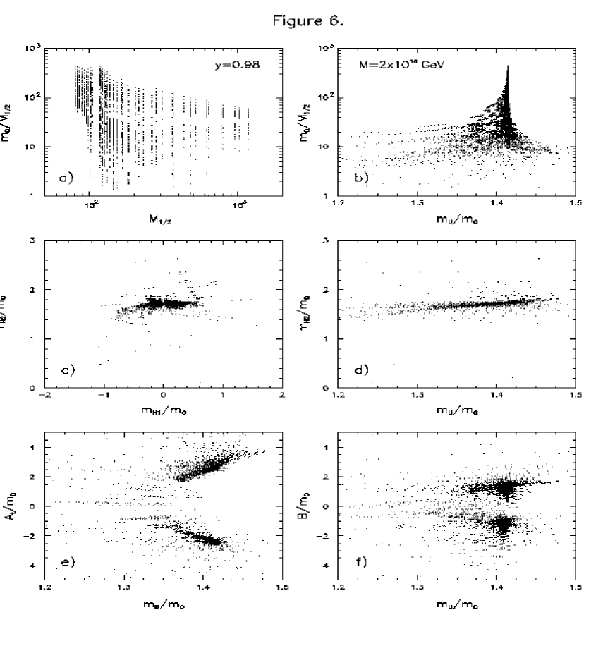
Figure 6: Soft supersymmetry breaking parameters at the scale $M=M_{GUT}=2\times 10^{16}$ GeV, for $y_{GUT}=0.98$ obtained by mapping the low-energy parameter space subject to the conditions specified in the section 4.

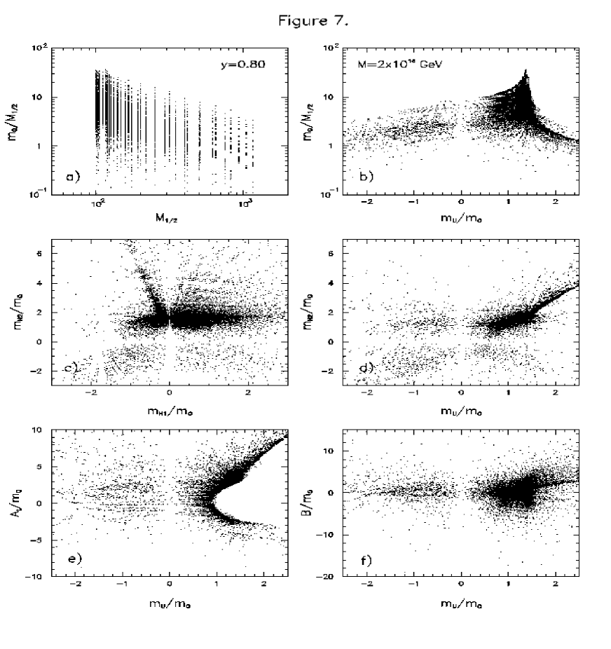
Figure 7: As in Fig. 6, but for $y_{GUT}=0.8$.

Figures 6 and 7 show the results for the soft supersymmetry breaking parameters at the scale  $M=M_{GUT}$,  obtained by mapping the whole low energy region shown in Figs. 3 and 4.  We plot

$$m_{K}\equiv{m^{2}_{K}(0)\over\sqrt{|m^{2}_{K}(0)|}},\;\;\;\;\;\;\;A_{t}\equiv A_{t}(0),\;\;\;\;\;\;\;B\equiv B(0),$$ (28)

for two different values of the top quark Yukawa coupling,  $y\simeq 0.98$  and   $0.8$.  Since the chargino mass is fixed, for any value of  $r=M_{2}/|\mu|$,  the values of  $M_{2}$  and  $\mu$  are uniquely determined (for any given sign of  $\mu$).  We have checked that the qualitative behaviour of the solutions do not strongly depend on the sign of  $\mu$.

Figure 6a shows that, for  $y\simeq 1$,  the characteristic third-generation squark scalar masses at the scale  $M_{GUT}$  must be, in general, much larger than the common gaugino masses. The stronger the deviation from the low-energy fixed-point relations, eqs. (19), the larger the value of  $m_{Q}/M_{1/2}$.  The strong correlations between the different scalar mass parameters at  $M_{GUT}$,  eq. (21), ensure the strong cancellations necessary to obtain low energy squark masses of order  $M_{1/2}$.  For values of  $y$ not very close to  $1$,  the resulting values of  $m_{Q}/M_{1/2}$  become smaller and the correlations are weaker. This behaviour is clearly illustrated in Fig. 7a  for  $y=0.80$.

In Fig. 6b we show the behaviour of  $m_{U}/m_{Q}$   for different values of  $M_{1/2}$  selected in our scan. A clear concentration of solutions around  $m_{U}/m_{Q}=\sqrt{2}$   appears. This concentration dilutes when we depart from the infrared fixed point solution for the top quark mass, as is clearly shown in Fig. 7b. Due to the relation of eq. (23), for a given stop spectrum, the values of  $m_{Q}/m_{U}$  are mainly governed by the size of  $M_{1/2}$.   For low values of  $M_{1/2}$,  the maximum value of  $m_{U}/m_{Q}$  is given by $\sqrt{2}$, while for all solutions with large values of  $M_{1/2}={\cal O}$(1 TeV) one has  $m_{U}/m_{Q}>\sqrt{2}$.  This is clearly seen in Figs 6b and 7b, where all solutions converge to   $m_{Q}/m_{U}=\sqrt{2}$  for large values of  $m_{Q}/M_{1/2}$.

In Figs 6c and 7c  we show the behaviour of the soft supersymmetry breaking Higgs mass parameters. Similarly to the relation between  $m_{U}$  and  $m_{Q}$,   it follows from eq. (23) that the hierarchy between   $m_{H_{2}}$  and  $m_{Q}$  is governed by the size of the gaugino masses. Values of  $m_{H_{2}}/m_{Q}\geq\sqrt{3}$  may only appear for large values of the gaugino masses, while low values always lead to  $m_{H_{2}}/m_{Q}\leq\sqrt{3}$.  For  $y\simeq 1$,  a strong concentration of solutions around the boundary value is observed. Solutions with negative values of  $m^{2}_{H_{1}}$,  associated with large values of  $\mu$,   are present in the data. For values of the lightest stop mass of order or below  $M_{Z}$,  a non-negligible stop mixing is in general necessary. For moderate values of  $\mu$   and  $M_{1/2}$,  values of  $A_{t}(t)$  appear, which violate relations (19). Therefore, from eqs. (6), it follows that close to the fixed point for the top quark mass,  $A_{t}$  becomes large. From eq. (2), it follows that, in this case,  $A_{t}$   dominates the renormalization group evolution of the scalar mass, implying the correlation  $A_{t}/m_{Q}\simeq\sqrt{6}$,  which is clearly observable in Fig. 6e. For lower values of  $y$,   as displayed in Fig. 7e,  $A_{t}$  ceases to dominate the evolution of the scalar mass parameters.

The behaviour of the solutions shown in Figs. 6 and 7 is just a reflection of the properties discussed above and shows the global tendency in the mapping of the low energy region selected by our criteria. The last important point we would like to discuss concerns the properties of the subregion, in the low-energy parameter space, that is consistent with simple patterns of the high-energy soft SUSY breaking parameters, such as universality or partial universality of scalar masses. It is clear from our earlier discussion that the closer is  $y$ to  $1$  the more restrictive such an Ansatz is.

In Figs 3 and 4  we show the regions, in the  $(\theta_{\tilde{t}},M_{\tilde{t}_{1}})$  and  $(M_{A},r)$  planes, which are consistent with the experimental constraints and can be obtained   a) with fully universal scalar masses at  $M_{GUT}$,  b) with  $m^{2}_{Q}=m^{2}_{U}=m^{2}_{H_{2}}$,   c) with  $m^{2}_{Q}=m^{2}_{U}$  ($SO(10)$-type boundary conditions). As expected from our qualitative analysis in section 3 and from Figs. 1 and 2,  such regions indeed exist, even for  $y\rightarrow 1$.   Cases a) and b) can only be realized with gaugino-like charginos and with large  $A_{t}$.  In the case c) we get both gaugino- and higgsino-like charginos (in agreement with the results displayed in Figs. 1 and 2) and the Higgs soft SUSY breaking masses tend to be ordered in such a way that  $m^{2}_{H_{2}}>m^{2}_{Q}>m^{2}_{H_{1}}$.   Comparison with contours in Figs. 2 shows that solutions with higgsino-like charginos fall into the region that gives  $R_{b}$  larger than in the SM by  $\delta R_{b}\sim 0.0010$.  Larger positive deviations from the Standard Model predictions for  $R_{b}$  demand both larger values of  $m_{Q}/M_{1/2}$  and soft supersymmetry breaking mass parameters with a hierarchy of masses close to the one given by eq. (21). Similar conclusions, although less sharp, hold also for  $y=0.80$.   We conclude that in the low-energy parameter space characterized by light chargino and stop there exists a subspace corresponding to the simple patterns of initial conditions discussed above which is consistent with the available experimental data. The hierarchy  $m_{0}\gg M_{1/2}$  must be, of course, present if the scalar masses at  $M_{GUT}$  are to satisfy   $m^{2}_{Q}\approx m^{2}_{U}\approx m^{2}_{H_{2}}$  or   $m^{2}_{Q}\approx m^{2}_{U}\approx m^{2}_{H_{2}}\approx m^{2}_{H_{1}}$   In the case of  $SO(10)$-type boundary conditions, the hierarchy   $m_{0}\gg M_{1/2}$  is also generically present although there can be also solutions with  $m_{0}\stackrel{{\scriptstyle<}}{{{}_{\sim}}}M_{1/2}$.

5. GAUGE-MEDIATED SCENARIOS OF SUSY BREAKING

Models in which supersymmetry breaking is transmitted to the observable sector through ordinary  $SU(3)\times SU(2)\times U(1)$   gauge interactions of the so-called messenger fields at scales   $M\ll M_{GUT}$  have recently attracted a lot of interest [2, 9, 25, 26, 27]. In general, these gauge-mediated models of SUSY breaking are characterized by two scales: the scale  $M$,  which is of the order of the average messenger mass and the scale  $\sqrt{F}$  of supersymmetry breaking. Since the physical messenger masses squared are given by

$$m_{\rm mess.}^{2}\simeq M^{2}\pm F,$$ (29)

one must have  $F<M^{2}$.  In the minimal models a lower bound on the scale  $M$,  $M\stackrel{{\scriptstyle>}}{{{}_{\sim}}}20$ TeV,  is set by the requirement   $M_{\tilde{\nu}}$, $M_{\tilde{e}_{R}}>M_{Z}/2$  [27]. In those models the ordinary “LSP” always decays into a gravitino (and an ordinary particle) whose mass is related to the scale  $\sqrt{F}$  by

$$m_{\tilde{G}}\simeq 4{\rm~{}eV}\times\left({\sqrt{F}\over 100~{}{\rm TeV}}\right)^{2}.$$ (30)

Since the decay length of the lightest neutral gaugino into photon and gravitino is approximately given by

$${\it l}\simeq 2\times 10^{-3}\times\left({\sqrt{F}\over 75~{}{\rm TeV}}\right)^{4},$$ (31)

it follows that, if  $\sqrt{F}\stackrel{{\scriptstyle<}}{{{}_{\sim}}}10^{6}$ GeV,  apart from missing energy, photons become a relevant signature for supersymmetry search at LEP and Tevatron colliders, because the lightest neutralino decays before leaving the detector. Such final photon states may be efficiently searched for at the Tevatron collider, and the absence of any spectacular signature in the existing  $\sim 100$ pb^-1  of data strongly disfavours chargino and stop masses below  100 GeV   [9]. Hence, the chargino and stop would be outside the reach of the LEP2 collider. Since our motivation is based on LEP2 physics, we consider here the scales  $M$  and  $\sqrt{F}$  such that the neutralino always decays only after leaving the detector. This leads to values  $\sqrt{F}\stackrel{{\scriptstyle>}}{{{}_{\sim}}}10^{6}$ GeV   and  $M\stackrel{{\scriptstyle>}}{{{}_{\sim}}}10^{7}$ GeV.  We have also analysed what happens for  $M\approx 10^{5}$ GeV  (usually considered in the context of gauge-mediated models [2, 25, 9]), and values of the stop and chargino masses consistent with the Tevatron bounds. We shall comment on this possibility at the end of this section.

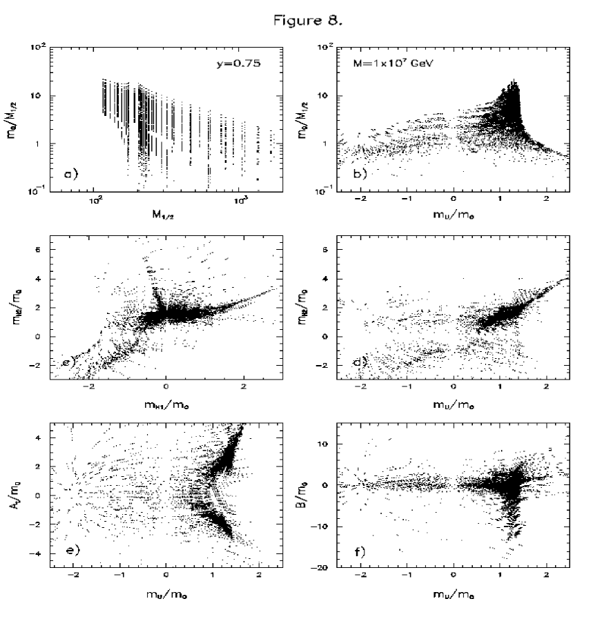
Figure 8: As in Fig. 6, but for $M=10^{7}$ GeV and $y(t)=0.75$.

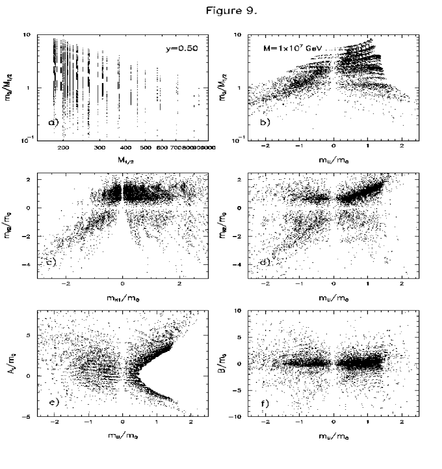
Figure 9: As in Fig. 8, but for $y(t)=0.50$.

Figures 8 and 9  show the solutions obtained for  $M=10^{7}$ GeV  and two different values of the auxiliary function  $y=0.75$  and  $y=0.50$,   which, for  $m_{t}=175$ GeV  and  $\alpha_{s}(M_{Z})=0.118$,  correspond to the low (1.2) and moderate (5.9)  $\tan\beta$  regimes, respectively. The variation with  $\tan\beta$  of the soft supersymmetry-breaking parameters is weaker than for   $M=M_{GUT}$,  reflecting the lower sensitivity to the GUT scale fixed-point solution.  The dependence on the actual value of   $y_{GUT}$  is weaker, since the auxiliary function  $y(t)$  always takes values smaller than  1.  For instance, for  $y_{GUT}=1$   ($M_{GUT}=2\times 10^{16}$ GeV)  and  $M=10^{7}$ TeV, we get  $y(t)\sim 0.70$.   As we explained before, since additional matter multiplets must be present at scales above the scale $M$,   a value of $y(t)\sim 0.75$ does not imply a breakdown of the perturbative consistency of the theory at scales below the grand unification scale. In this case the violation of the sum rules, eq. (19), is not associated with an enhancement of the values of the parameters at the scale  $M$.  From the analysis of our equations, for these low values of  $M$  and  $y(t)$,  it follows that the values of the soft terms at the scale  $M$  tend to reflect the pattern observed at the  $M_{Z}$  scale. Still, the larger  $y(t)$  the closer we are to the effects discussed earlier and the larger the modification of the pattern at  $M_{Z}$  with respect to the initial conditions. Indeed, as can be seen from the comparison of Figs. 7 and 8, the qualitative behaviour of the solutions for  $y=0.75$   is very similar to the one obtained in the gravity mediated supersymmetry breaking scenario for  $y=0.80$.

Due to the smaller renormalization group running effects and the fact that  $\eta_{Q}\simeq 1.6$,  the ratio   $m_{Q}/M_{1/2}$  reflects the chosen values of the left-handed stop parameter and the gluino mass at low energies, increasing for lower values of  $M_{1/2}$,  as is clearly shown in Figs. 8a and 9a. More interesting is the behaviour of  $m_{U}/m_{Q}$  displayed in Figs. 8b and 9b. The concentration of solutions around   $m_{U}/m_{Q}\simeq\sqrt{2}$  is still visible at low values of $\tan\beta$, but it disappears for low values of $y$. Indeed, for $y=0.50$ the ratio  $m_{U}/m_{Q}$  tends, in general, to be lower than   1.  However, values of  $m_{U}/m_{Q}$  of order  1  can also appear as possible solutions in this scenario. Hence, a light stop is not necessarily in conflict with models of supersymmetry breaking in which   $m_{U}/m_{Q}\simeq 1$  at the scale  $M\sim 10^{7}$ GeV. This is true for both values of  $y$,   although it is easier to accommodate  $m_{U}/m_{Q}$  of order  1  for low values of  $\tan\beta$  (larger values of  $y$).   For $y=0.5$, however,  $m_{U}/m_{Q}\sim 1$  implies large values of  $A_{t}$   and/or large values of  $M_{A}$.

For  $M=10^{7}$ GeV,  instead of going into further detail of the mapping of the full allowed low-energy region, it is more interesting to check where there are points that correspond to initial values of the soft parameters, which are generic for the gauge-mediated scenarios of SUSY breaking.

We impose the most universal conditions in the following way. In the more restrictive version, from

$$M_{1/2}={\alpha_{3}(0)\over 4\pi}\Lambda$$ (32)

we extract  $\Lambda=F/M$  and then  $m^{2}_{Q}(0)$  and  $m_{U}^{2}(0)$   are required to be no more than 10% off from the values

$$m^{2}_{Q~{}g.m.} = 2\Lambda^{2}\left[{4\over 3}\left({\alpha_{3}(0)\over 4\pi}\right)^{2}+{3\over 4}\left({\alpha_{2}(0)\over 4\pi}\right)^{2}+{1\over 60}\left({\alpha_{1}(0)\over 4\pi}\right)^{2}\right]$$

$$m^{2}_{U~{}g.m.} = 2\Lambda^{2}\left[{4\over 3}\left({\alpha_{3}(0)\over 4\pi}\right)^{2}+{4\over 15}\left({\alpha_{1}(0)\over 4\pi}\right)^{2}\right]$$ (33)

predicted in such models [2] . In the less restrictive version,  $m_{Q}^{2}(0)$  and   $m^{2}_{U}(0)$  must only satisfy (within 10%) the relation following from eq. (33) and we do not impose condition (32). We do not constrain  $m^{2}_{H_{1,2}}(0)$  or  $A_{t}$.   In gauge-mediated models the prediction  $A_{t}\sim 0$  is also quite general, but we prefer to see the regions defined by the conditions specified above and to check the corresponding values of  $m^{2}_{H_{1,2}}(0)$   and  $A_{t}$.

In Figs. 5a,b we show the contours consistent with experimental constraints and mark the regions defined by the above conditions (more and less restrictive cases are shown by dark stars and white rhombs, respectively), whereas in Fig. 10  we show the corresponding ratios  $h_{1,2}$  of the actual values of  $m^{2}_{H_{1,2}}(0)$  obtained from the low-energy mapping to the values  $m^{2}_{H_{1,2}~{}g.m.}$   predicted in the minimal models of gauge-mediated symmetry breaking (with  $\Lambda$  determined from eq. (32) or (33) in the more and less restrictive cases, respectively):

$$m^{2}_{H_{1,2}~{}g.m.}=2\Lambda^{2}\left[{3\over 4}\left({\alpha_{2}(0)\over 4\pi}\right)^{2}+{3\over 20}\left({\alpha_{1}(0)\over 4\pi}\right)^{2}\right].$$ (34)

Also, the obtained values of  $A_{t}$  and  $B$  are displayed. From Fig. 10, it is clear that a light stop is always associated with values of  $m_{H_{2}}^{2}(0)$  very large with respect to the ones that would be obtained in the minimal models. However, because of the uncertainty in the values of these parameters associated with the physics involved in the solution to the  $\mu$  problem in the gauge-mediated supersymmetry-breaking models [26], such large values of  $m^{2}_{H_{2}~{}g.m.}$  are not necessarily inconsistent in this context. The value of  $A_{t}$  must be, in general, large, a reflection of the small hierarchy of scales and the large values of the stop mixing necessary to generate a light stop. Smaller values of  $A_{t}$  can only be obtained by increasing the value of   $m^{2}_{H_{2}}$  and, hence, the mass of the $CP$-odd Higgs boson. In fact, for $m_{U}(0)\simeq m_{Q}(0)$, $A_{t}\simeq 0$, we obtain

$$M_{A}^{2} = {M_{Z}^{2}\over 2}\left(\tan^{2}\beta-1\right)+\left[\mu^{2}+m_{Q}^{2}(t)\;{6-7y\over y}+m_{U}^{2}(t)\;{5y-6\over y}\right.$$ (35)

$$+ \left.M_{1/2}^{2}\left(\eta_{Q}\;{7y-6\over y}+\eta_{U}\;\frac{6-5y}{y}+\eta_{H_{2}}-\hat{\eta}+y\hat{\xi}^{2}\right)\right]\left(\tan^{2}\beta+1\right).$$

It is easy to show that the  $M_{1/2}^{2}$  coefficient is positive for any value of  $M$  and  $y$.  It follows from the above expression that, for  $y<0.8$,  values of  $m_{U}^{2}\ll m_{Q}^{2}$  can only be obtained for large values of  $M_{A}$,  particularly for large values of  $\tan\beta$.   Indeed, in the more restrictive case, for  $y=0.75$ (0.50),  i.e. for   $\tan\beta$  small (intermediate), solutions with  $A_{t}\sim 0$   are possible only for very large values of  $M_{A}$,  $M_{A}\stackrel{{\scriptstyle>}}{{{}_{\sim}}}1~{}(5)$ TeV,   and  $h_{1,2}\sim{\cal O}(15)$.   In the less restrictive case, for  $y=0.75$,  solutions with  $A_{t}\sim 0$   are possible already with  $M_{A}\stackrel{{\scriptstyle>}}{{{}_{\sim}}}800$ GeV (they require, however,   $h_{1,2}\sim{\cal O}(20)$).  For  $y=0.50$,  even in the less restrictive case, they require extremely large values of  $M_{A}$  ($M_{A}\stackrel{{\scriptstyle>}}{{{}_{\sim}}}3$ TeV) and   $h_{1,2}\stackrel{{\scriptstyle>}}{{{}_{\sim}}}{\cal O}(50)$.

Let us end this section by mentioning what happens for  $M\approx 10^{5}$ GeV   and values of the chargino and stop masses slightly above the present Tevatron bounds. Notice that, although this range of masses is outside the reach of LEP2, it is still consistent with the requirements of electroweak baryogenesis in the MSSM. In this case, for values of   $\tan\beta$  similar to the ones chosen for  $M=10^{7}$ GeV,  one obtains the values  $y=0.55$  and  $y=0.35$,   respectively, while the coefficients associated with the dependence of the scalar masses on the gaugino ones is reduced by a factor  2   with respect to the ones obtained for  $M=10^{7}$ GeV.  Since for low values of  $\eta_{K}$,  the overall properties are governed by the value of  $y$,  the solutions for  $y=0.55$  resemble those obtained for   $y=0.50$  at  $M=10^{7}$ GeV.  The bounds on the $CP$-odd mass necessary for obtaining a light stop in the gauge-mediated scenario are somewhat weaker, since there is a  $\tan\beta$  enhancement associated with this value, as is clear from eq. (35). Hence, for  $y=0.55$,  in the most restrictive case a light stop may only be obtained for $CP$-odd masses of the order of   2 TeV,  while in the less restrictive case, masses of order  900 GeV   are necessary. For  $y=0.35$,  the bounds are raised to  6 TeV  and  5 TeV, respectively.

6. CONCLUSIONS

In this paper we have discussed the mapping to high energies of the low energy region of the MSSM parameter space, characterized by the presence of a light stop and light chargino. The parameter space considered is consistent with present experimental constraints, such as precision tests, the lower bound on the Higgs boson mass and  $BR(b\rightarrow s\gamma)$  and therefore of special interest for physics at LEP2 and the Tevatron colliders. For heavy top quark and small  $\tan\beta$,  the global pattern of the mapping is determined by the proximity of the top-quark Yukawa coupling to its IR fixed-point value and by the assumed scale at which supersymmetry breaking is transmitted to the observable sector. The general pattern of this mapping is the dominance of the scalar masses (over the gaugino mass) in the supersymmetry breaking and the strong correlation between the soft SUSY breaking mass parameters   $m^{2}_{Q}$,  $m^{2}_{U}$  and  $m^{2}_{H_{2}}$.  Moreover, we have identified the conditions that are necessary for the spectrum to be consistent with a simple Ansatz such as universality (or partial universality) of the high energy values for the scalar masses. In particular, the  $SO(10)$-type initial conditions, with universal left- and right-handed squark masses, but with non-universal Higgs masses, are compatible with an interesting subregion of the considered parameter space. In the scenario in which the supersymmetry breaking is transferred to the observable sector via gravitational interactions, the conditions for such simple patterns are easier to satisfy away from the IR fixed point. On the contrary, for low values of the messenger masses, these patterns are easily obtained for small   $\tan\beta$  and values of the top quark Yukawa couplings associated with large values of  $h_{t}$  at  $M_{GUT}$.  In the latter case the considered low energy spectra can be consistent with the typical boundary conditions for the squark and gaugino appearing in gauge-mediated supersymmetry breaking. However, consistency with with another generic prediction of those scenarios,  $A_{t}\sim 0$,   can be achieved only for extremely large values of the $CP$-odd Higgs boson mass.

Acknowledgements

M.C. and C.W. would like to thank the Aspen Center for Physics, where part of this work has been done.

P.H.Ch. would like to thank Prof. H. Haber and the Santa Cruz Institute for Particle Physics for hospitality. His work and the work of S.P. were partly supported by the joint U.S.–Polish Maria Skłodowska Curie grant.

M.O. thanks the INFN Sezione di Torino where part of this work has been done. His work was partly supported by the Deutsche Forschungsgemeinschaft under grant SFB–375/95 and by the European Commission TMR programmes ERBFMRX-CT96-0045 and ERBFMRX-CT96-0090.

APPENDIX

Here we collect formulae for various factors appearing in the solutions to the RGEs. Solutions for the soft masses contain the following functions of the gauge coupling constants:

$$\xi_{j}(t)=I\left[\sum_{i}\frac{M_{i}(0)}{M_{1/2}}\frac{a_{j}^{i}\alpha_{i}^{2}(t)}{\alpha_{i}(0)}\right]$$ (36)

$$\eta_{K}(t)=I\left[\sum_{i}\frac{M_{i}^{2}(0)}{M_{1/2}^{2}}\frac{d_{K}^{i}\alpha_{i}^{3}(t)}{\alpha_{i}^{2}(0)}\right]$$ (37)

$${\hat{\xi}}(t)=H\left[\sum_{i}\frac{M_{i}(0)}{M_{1/2}}\frac{a^{i}_{u}\alpha_{i}^{2}(t)}{\alpha_{i}(0)}\right]$$ (38)

$${\hat{\eta}}(t)=H\left[\sum_{i}\frac{M_{i}^{2}(0)}{M_{1/2}^{2}}\frac{\overline{d}^{i}\alpha_{i}^{3}(t)}{\alpha_{i}^{2}(0)}\right]+H\left[\sum_{i}\frac{M_{i}(0)}{M_{1/2}}\frac{\overline{d}^{i}\alpha_{i}^{2}(t)}{\alpha_{i}(0)}\xi_{u}(t)\right],$$ (39)

where the coefficients  $a^{i}_{j}$  and  $d^{i}_{K}$   read:  $a_{u}^{i}=(13/15,3,16/3)$,   $a_{d}^{i}=(7/15,3,16/3)$,  $a_{e}^{i}=(3/5,3,0)$  ($\xi_{B}=\xi_{e}$);   $d_{Q}^{i}=(1/15,3,16/3)$,  $d_{U}^{i}=(16/15,0,16/3)$,   $d_{D}^{i}=(4/15,0,16/3)$,  $d_{L}^{i}=d^{i}_{H_{1}}=d^{i}_{H_{2}}=(3/5,3,0)$,   $d_{E}^{i}=(12/5,0,0)$;   $\overline{d}^{i}\equiv d^{i}_{Q}+d^{i}_{U}+d^{i}_{H_{2}}$  and  $I$,  and  $H$   are defined by:

$$I[f(t)]=\int_{0}^{t}f(t^{\prime})dt^{\prime}$$ (40)

$$H[f(t)]=\int_{0}^{t}f(t^{\prime})dt^{\prime}-\frac{1}{F(t)}\int_{0}^{t}F(t^{\prime})f(t^{\prime})dt^{\prime}$$ (41)

with  $F(t)$  given by eqs. (11). The factors  $M_{i}(0)/M_{1/2}\neq 1$  appear because we do not assume exact gauge coupling unification and, by convention,  $M_{1/2}\equiv M_{3}(0)$.   Parameters  $\xi_{i}$  and  $\eta_{K}$  can be computed analytically. Parameters  $\hat{\xi}$  and  $\hat{\eta}$  require numerical integration. We give below (using the assumption (25)) their typical values for few scales  $M$  and three values of  $\alpha_{3}$.   For other values of   $\alpha_{3}$,  $\hat{\xi}$  and  $\hat{\eta}$  can be easily obtained by interpolation.

Table 1. Typical  $\hat{\xi}$  values

$\hat{\xi}$		$\,M$ [GeV]
		$4\times 10^{16}$	$2\times 10^{16}$	$1\times 10^{16}$	$1\times 10^{10}$	$1\times 10^{7}$	$1\times 10^{5}$
	0.115	2.22	2.16	2.10	1.08	0.640	0.374
$\alpha_{3}$	0.120	2.29	2.23	2.17	1.11	0.663	0.388
	0.125	2.36	2.30	2.23	1.15	0.686	0.402

Table 2. Typical  $\hat{\eta}$  values

$\hat{\eta}$		$\,M$ [GeV]
		$4\times 10^{16}$	$2\times 10^{16}$	$1\times 10^{16}$	$1\times 10^{10}$	$1\times 10^{7}$	$1\times 10^{5}$
	0.115	12.7	12.1	11.6	4.16	1.10	0.987
$\alpha_{3}$	0.120	13.4	12.8	12.3	4.39	2.10	1.04
	0.125	14.1	13.5	12.9	4.63	2.22	1.09

Table 3. Typical  $\xi_{u}$  values

$\xi_{u}$		$\,M$ [GeV]
		$4\times 10^{16}$	$2\times 10^{16}$	$1\times 10^{16}$	$1\times 10^{10}$	$1\times 10^{7}$	$1\times 10^{5}$
	0.115	3.94	3.84	3.75	2.03	1.24	0.736
$\alpha_{3}$	0.120	4.07	3.97	3.88	2.10	1.29	0.764
	0.125	4.20	4.10	4.01	2.17	1.33	0.792

Table 4. Typical  $\xi_{B}$  values

$\xi_{B}$		$\,M$ [GeV]
		$4\times 10^{16}$	$2\times 10^{16}$	$1\times 10^{16}$	$1\times 10^{10}$	$1\times 10^{7}$	$1\times 10^{5}$
	0.115	0.614	0.590	0.566	0.210	0.102	0.050
$\alpha_{3}$	0.120	0.605	0.581	0.557	0.206	0.099	0.049
	0.125	0.597	0.573	0.549	0.202	0.097	0.047

Table 5. Typical  $\eta_{Q}$  values

$\eta_{Q}$		$\,M$ [GeV]
		$4\times 10^{16}$	$2\times 10^{16}$	$1\times 10^{16}$	$1\times 10^{10}$	$1\times 10^{7}$	$1\times 10^{5}$
	0.115	6.87	6.65	6.44	2.85	1.54	0.836
$\alpha_{3}$	0.120	7.27	7.04	6.81	3.01	1.62	0.876
	0.125	7.69	7.44	7.19	3.17	1.70	0.917

Table 6. Typical  $\eta_{U}$  values

$\eta_{U}$		$\,M$ [GeV]
		$4\times 10^{16}$	$2\times 10^{16}$	$1\times 10^{16}$	$1\times 10^{10}$	$1\times 10^{7}$	$1\times 10^{5}$
	0.115	6.42	6.22	6.03	2.74	1.50	0.817
$\alpha_{3}$	0.120	6.84	6.62	6.41	2.90	1.58	0.858
	0.125	7.26	7.03	6.81	3.06	1.66	0.900

Table 7. Typical  $\eta_{H_{2}}$  values

$\eta_{H_{2}}$		$\,M$ [GeV]
		$4\times 10^{16}$	$2\times 10^{16}$	$1\times 10^{16}$	$1\times 10^{10}$	$1\times 10^{7}$	$1\times 10^{5}$
	0.115	0.561	0.529	0.499	0.128	0.049	0.020
$\alpha_{3}$	0.120	0.544	0.513	0.484	0.123	0.047	0.019
	0.125	0.530	0.499	0.471	0.118	0.045	0.018

Figure 1: $\Delta_{m^{2}}$ defined in eqs. (19),(22) as a function of $r\equiv M_{2}/|\mu|$  for  $M_{A}=1000$ (solid lines),   $750$ (dashed), $500$ (dotted) and $250$ (dash-dotted) GeV.  Different lines of the same type correspond to $M_{\tilde{t}_{1}}=1000$ (upper), $750$ (middle) and $500$ (lower) GeV. Cases with positive and negative $\mu$ are shown in a) and b) respectively. Values of  $m_{t}=175$ GeV,  $\tan\beta=1.6$,   $m_{C^{+}}=90$ GeV  and  $M_{\tilde{t}_{2}}=60$ GeV are taken.

Figure 2: a.  Contours of $\Delta_{A}=50$ (internal solid lines) and 100 GeV(external ones) in the plane $(r,~{}\theta_{\tilde{t}})$  for $M_{\tilde{t}_{1}}=1000$ GeV (for positive and negative values of  $\mu$  in the upper and lower panels respectively). Regions excluded by  $M_{h}>60$ GeV (horizontal lines)  and  $0.98\times 10^{-4}<BR(b\rightarrow s\gamma)<3.66\times 10^{-4}$  for  $M_{A}=1000$, 500 and 250 GeV  are marked by dashed, dot-dashed, and dot-dot-dashed lines respectively (contours of $\Delta_{A}$ are  $M_{A}$ independent, see eq. (22)). Dotted contours show values of   $\delta R_{b}\times 10^{4}$.  Other parameters as in Fig. 1.

Figure 2: b.  As in Fig. 2a, but for $M_{\tilde{t}_{1}}=500$ GeV.

Figure 3: a.  Regions in the  $(r,M_{A})$   plane allowed by experimental constraints listed in the text (for positive and negative values of  $\mu$  in the upper and lower panels respectively) for  $\tan\beta=1.6$  (corresponding for   $M_{GUT}=2\times 10^{16}$ GeV  to  $y=0.98$).   Regions above the dashed lines are allowed by  $M_{h}>60$ GeV  and   $BR(b\rightarrow s\gamma)$.  In regions above the solid lines, in addition,  $\chi^{2}<\chi^{2}_{best~{}SM}+2$ (see the text). The black star shows the point that can be obtained with fully universal boundary conditions at  $M_{GUT}$ (i.e. with $m^{2}_{Q}(0)$, $m^{2}_{U}(0)$, $m^{2}_{H_{1}}(0)$ and $m^{2}_{H_{2}}$  all equal within 10%). The white rhombs denote points that can be realized with $m^{2}_{Q}(0)$, $m^{2}_{U}(0)$, $m^{2}_{H_{2}}(0)$ equal and the dots correspond to points that require $SO(10)$-type initial values (i.e. $m^{2}_{Q}(0)=m^{2}_{U}(0)$ within 10%). All marked points are consistent with our experimental cuts. Values of the other parameters as in Fig. 1.

Figure 3: b.  As in Fig. 3a, but in the  $(M_{\tilde{t}_{1}},~{}\theta_{\tilde{t}})$ plane. Allowed regions are inside marked contours.

Figure 4: a.  As in Fig. 3a,  but for  $\tan\beta=2.8$  (corresponding for  $M_{GUT}=2\times 10^{16}$ GeV  to  $y=0.80$).

Figure 4: b.  As in Fig. 4a, but in the   $(M_{\tilde{t}_{1}},~{}\theta_{\tilde{t}})$ plane.

Figure 5: a.  As in Fig. 3a,  but for  $\tan\beta=1.2$  (corresponding, for  $M=10^{7}$ GeV,  to  $y=0.75$). The black stars (white rhombs) show the points that can be obtained with more (less) restrictive boundary conditions at  $M=10^{7}$ GeV (see the text for explanation).

Figure 5: b.  As in Fig. 5a, but in the  $(M_{\tilde{t}_{1}},~{}\theta_{\tilde{t}})$ plane.

Figure 10: Ratio ($h_{1,2}$) of the squared Higgs boson mass parameters, $m_{H_{1,2}}^{2}(0)$, to the ones predicted in gauge-mediated supersymmetry breaking models, for the case of minimal relations between the squark and gaugino masses (left) and for the unrestricted case (right). The behaviour of the soft supersymmetry breaking parameters $A_{t}$ and $B$ at the scale $M=10^{7}$ GeV is also shown here.

References

- [1] H.-P. Nilles Phys. Rep. 110C (1984) 1.
-
[2]
M. Dine, W. Fischler, M. Srednicki Nucl. Phys.
B189 (1981) 575,
S. Dimopoulos, S. Raby Nucl. Phys. B192 (1981) 353,
L. Alvarez-Gaumé, M. Claudson, M. Wise Nucl. Phys. B207 (1982) 96,
M. Dine, A. Nelson Phys. Rev. D48 (1993) 1277,
M.. Dine, A. Nelson, Y. Shirman Phys. Rev. D51 (1995) 1362,
M. Dine, A. Nelson, Y. Nir, Y. Shirman Phys. Rev. D53 (1996) 2658. - [3] The LEP Electroweak Working Group, CERN preprint LEPEWWG/96-02.
-
[4]
J. Ellis, G.L. Fogli, E. Lisi Z. Phys. C69 (1996)
627, preprint CERN–TH/96–216 (hep-ph/9608329),
P. Chankowski, S. Pokorski Phys. Lett. B356 (1995) 307, Acta Phys. Pol. B27 (1996) 933 (hep-ph/9509207). - [5] G. Altarelli, R. Barbieri, F. Caravaglios Nucl. Phys. B405 (1993) 3, Phys. Lett. 314B (1993) 357.
- [6] J. Ellis, G.L. Fogli, E. Lisi Nucl. Phys. B393 (1993) 3, Phys. Lett. B324 (1994), 173, 333B (1994) 118.
- [7] P.H. Chankowski, S. Pokorski Phys. Lett. 366B (1996) 188.
- [8] P.H. Chankowski, S. Pokorski Nucl. Phys. B475 (1996) 3.
- [9] S. Ambrosanio et al. Phys. Rev. Lett. 76 (1996) 3498, Phys. Rev. D54 (1996) 5395.
- [10] M. Drees et al. preprint MADPH-96-944 (hep-ph/9605447).
- [11] M. Boulware, D. Finnell Phys. Rev. D44 (1991) 2054.
-
[12]
G.L. Kane, C. Kolda, J.D. Wells
Phys. Lett. 338B (1994) 219,
G.L. Kane, R.G. Stuart, J.D. Wells Phys. Lett. 354B (1995) 350. -
[13]
J. Rosiek Phys. Lett. 252B (1990) 135,
A. Denner et al. Z. Phys. C51 (1991) 695,
D. Garcia, R. Jimenéz, J. Solà Phys. Lett. 347 (1995) 309, 321, E 351B (1995) 602,
D. Garcia, J. Solà Phys. Lett. 354B (1995) 335, 357B (1995) 349. -
[14]
K.G. Chetyrkin, M. Misiak, M. Münz to be published,
private communication of M. Misiak,
C. Greub, T. Hurth, D. Wyler Phys. Rev. D54 (1996) 3350,
C. Greub, T. Hurth talk given at 1996 Meeting of the Division of Particles and Fields of the American Physical Society, Minneapolis, August 1996 (hep-ph/9608449). -
[15]
D. Pierce, A. Papadopoulos Nucl. Phys. B430
(1994) 278,
D. Pierce, J. Bagger, K. Matchev, R.-J. Zhang preprint SLAC-PUB-7180 (hep-ph/9606211),
A. Donini Nucl. Phys. B467 (1996) 3. - [16] J. Bagger, S. Dimopoulos, E. Masso Phys. Rev. Lett. 55 (1985) 920.
- [17] M. Olechowski, S. Pokorski Phys. Lett. 257B (1991) 388.
- [18] M. Carena et al. Nucl. Phys. B369 (1992) 33.
-
[19]
S. Dimopoulos, L.J. Hall, S. Raby Phys. Rev. Lett. 68
(1992) 1984; Phys. Rev. D45 (1992) 4192,
V. Barger, M. Berger, P. Ohmann, R.J.N. Phillips Phys. Lett. 314B (1993) 351,
V. Barger, M. Berger, P. Ohmann Phys. Rev. D47 (1993) 1093,
G.W. Anderson, S. Raby, S. Dimopoulos, L. Hall Phys. Rev. D47 (1993) 3702,
M. Carena, S. Pokorski, C.E.M. Wagner, Nucl. Phys. B406 (1993) 59. - [20] H. Arason et al. Phys. Rev. D46 (1992) 3945.
- [21] M. Carena, M. Olechowski, S. Pokorski, C.E.M. Wagner Nucl. Phys. B419 (1994) 213.
-
[22]
M. Carena, M. Quiros, C.E.M. Wagner
Phys. Lett. 380B (1996) 81,
J.R. Espinosa Nucl. Phys. B475 (1996) 273,
D. Delepine, J.M. Gerard, R. Gonzalez Felipe, J. Weyers preprint UCL-IPT-96-05 (hep-ph/9604440). - [23] P. Huet, A.E. Nelson Phys. Rev. D53 (1996) 4578.
-
[24]
R. Hempfling Ph.D. Thesis, UCSC preprint SCIPP 92/28 (1992);
J.L. Lopez, D.V. Nanopoulos Phys. Lett. 266B (1991) 397. -
[25]
K.S. Babu, C. Kolda, F. Wilczek preprint IASSNS-HEP-96-55
(hep-ph/9605408),
S. Dimopoulos, S. Thomas, J.D. Wells, preprint SLAC-PUB-7237 (hep-ph/9609434). - [26] G. Dvali, G.F. Giudice, A. Pomarol preprint CERN-TH/96-61 (hep-ph/9603238).
- [27] S. Dimopoulos, G.F. Giudice preprint CERN-TH/96-171 (hep-ph/9607225).