hep-ph/9610468

UCSD-TH-96-27

October 1996

Bounds on Long-Lived Relics from Diffuse Gamma Ray Observations
Graham D. Kribs

Randall Physics Laboratory, University of Michigan,
Ann Arbor, MI 48109-1120

I.Z. Rothstein

Dept. of Physics, UCSD, La Jolla, CA 92122

We place bounds on long-lived primordial relics using measurements of the diffuse gamma ray spectrum from EGRET and COMPTEL. Bounds are derived for both radiative and hadronic decays with stronger bounds applying for the latter decay mode. We present an exclusion plot in the relic density–lifetime plane that shows nontrivial dependence on the mass of the relic. The violations of scaling with mass are a consequence of the different possible scattering processes which lead to differing electromagnetic showering profiles. The tightest bounds for shorter lifetimes come from COMPTEL observations of the low energy part of the spectrum, while for longer lifetimes the highest observable energy at EGRET gives the tightest bounds. We discuss the implications of the bounds for dark matter candidates as well as relics that have a mass density substantially below the critical density. These bounds can be utilized to eliminate models that contain relics with lifetimes longer than $10^{-4}$ times the age of the universe.

1 Introduction

While the standard model of particle physics has passed all experimental tests to date, it lacks a particle candidate that could provide the dark matter of the universe as expected from astronomical observations. Furthermore, our present understanding of structure formation seems to indicate that some fraction of the dark matter should be “cold”, so as to generate the proper power spectrum. Such dark matter candidates are quite common in many extensions of the standard model. Indeed, many models predict long lived relics that may or may not be dark matter candidates. Long lifetimes for heavy relics, where by “long” we mean within several orders of magnitude of the age of the universe may arise in many models which have symmetries that are only broken at short distances. Thus it is interesting to investigate the observational signatures of such long lived relics in an effort to rule out classes of models.

In this paper we study the signatures of particles with lifetimes comparable to the age of the universe. Such particles could play a role in solving the dark matter problem, but we will not confine our analysis to dark matter candidates. The inclusion of long lived heavy ($M_{\scriptscriptstyle X}\mathrel{\>{\hbox{\raise 1.50696pt\hbox{$>$}}\kern-3.8889pt\kern-3.8889pt\hbox{\lower 2.79857pt\hbox{$\sim$}}}\>}50~{}{\rm GeV}$) particles necessitates an extension of the standard model. These relics could be technibaryons in technicolor models or the lightest supersymmetric partner in an R-parity violating supersymmetric extension of the standard model. The bounds found here are model independent and depend on only three parameters: the mass $M_{\scriptscriptstyle X}$, the lifetime $\tau_{\scriptscriptstyle X}$ and the radiative or hadronic branching ratio times the relic density $B\cdot\eta_{\scriptscriptstyle X}$, with $\eta_{\scriptscriptstyle X}\equiv n_{\scriptscriptstyle X}/n_{\gamma}$. Given any model, it is possible to calculate the relic density using standard techniques leading to bounds on couplings as well as masses.

Our exclusion bounds are derived by considering the direct observation of the gamma rays produced in the decay process. In general, the predicted observed spectrum will differ greatly from the decay spectrum due to redshifting and scattering in the early universe. The final spectrum can be compared to the EGRET and COMPTEL data leading to the exclusion plots presented here.

Previous investigations [1, 2, 3, 4, 5] of the gamma ray spectra produced by long lived relics have concentrated on radiative decays into either photons or charged particles. We consider both radiative and hadronic decays, including the effects of photon–photon scattering and $e^{+}e^{-}$ pair production. There are reasons to believe that hadronic decays are more compelling. First, the hadronic branching ratio of the relics is expected to be of order one, unless there is a symmetry which forbids such decays. Radiative decays usually arise at the one loop level and so one would expect smaller branching ratios. Second, hadronic decays produce more photons in the softer part of the spectrum due to fragmentation, which produces a large number of pions that decay to two photons. Thus, as opposed to the case of radiative decay, we expect the non-scattered spectra to have more photons at smaller energies (i.e. $E_{\gamma}\ll M_{\scriptscriptstyle X}$). Since the diffuse photon background spectrum is well measured only up to $10$ GeV, we would naively expect our bounds to apply to larger mass relics $M_{\scriptscriptstyle X}\geq{\cal O}(10^{3})$ GeV for hadronic decays but not for radiative decays. However, bounds derived from radiative decays of large mass relics can be obtained if a reprocessing mechanism to lower the photon energy is active. Such mechanisms begin operating once injected photon energies are above about $23$ GeV where radiative decays can potentially compete with hadronic decays and produce large numbers of photons at low energy for masses larger than roughly $50$ GeV. Thus, a complete calculation is necessary to determine the bound for a given mode of decay, as we present here.

It should be noted that some of the bounds derived here will overlap those coming from structure formation arguments in the part of parameter space where the relic density is of the order of the critical density. Radiative decay can lead to a radiation dominated epoch after recombination that would drastically distort the observed power spectrum. Thus the shorter lifetimes considered here could lead to such distortions, but we will not consider these effects.

2 Electromagnetic Cascades in the Early Universe

A high energy photon injected in the early universe will, in general, scatter. Since there are many scattering processes possible, the nature of the scattering is strongly dependent on the redshift at which the photon is injected as well as its energy. Each process has a characteristic optical depth which determines its relevance to the evolution of the photon. The relevant processes were investigated in detail by Zdziarski and Svensson in Ref. [6]. The processes include: $e^{+}e^{-}$ pair production (PP), photon–photon scattering (GG), Compton scattering and pair production off of matter (PPM). Figure 1 (derived from [6]) divides the redshift energy plane into regions labeled by the process that dominates in a particular part of the graph. The photons always have injected energies, $E_{\gamma}\mathrel{\>{\hbox{\raise 1.50696pt\hbox{$>$}}\kern-3.8889pt\kern-3.8889pt\hbox{\lower 2.79857pt\hbox{$\sim$}}}\>}100$ MeV, which is obviously true of radiative decays of heavy relics and is also true of hadronic decays due to a cutoff in the spectrum at $E_{\gamma}=m_{\pi}/2$. Therefore, the mechanisms for rescattering photons with energies below about $100$ MeV are irrelevant to our analysis. Details of the spectra and cutoffs are described in the following sections.

Given the initial energy of the photon and the redshift at which it was injected, the progress of the injected photon can be tracked by moving horizontally across Fig. 1. For large enough photon energies, the time scale for scattering is short compared to the expansion rate of the universe, so we may neglect any vertical motion until we reach the region where Compton scattering dominates (not shown; to the left of the left edge of the graph) or where the photon reaches the point where its optical depth drops below one. In the limit that the photon energy is much smaller than the mass of the electron (Thompson limit), the cross section for Compton scattering is independent of energy. When the photons reach the region of the plot dominated by Compton scattering in the Thompson limit, the photons will eventually be in kinetic equilibrium with the thermal bath leading to a finite chemical potential for the photons. The resulting distortion of the precisely measured microwave background leads to bounds on the injection of low-energy photons prior to recombination ($z\simeq 1300$), as discussed in Ref. [4]. For photons with redshifts in the range $10^{3}\mathrel{\>{\hbox{\raise 1.50696pt\hbox{$<$}}\kern-3.8889pt\kern-3.8889pt\hbox{\lower 2.79857pt\hbox{$\sim$}}}\>}z\mathrel{\>{\hbox{\raise 1.50696pt\hbox{$<$}}\kern-3.8889pt\kern-3.8889pt\hbox{\lower 2.79857pt\hbox{$\sim$}}}\>}10^{6}$, the electromagnetic cascades result in the production of ³He and D via the disintegration of ⁴He. Thus, there will be even more stringent bounds for this range of redshifts coming from limits on primordial abundances of light elements [7, 8, 4]. Here we concern ourselves with bounds coming from direct observations of gamma rays, and therefore we will be interested in photons whose life begins in the region dominated by pair production or photon–photon scattering after the epoch of recombination. Such photons will eventually reach the region of the plot where the optical depth drops below one and can be directly detected.

Pair production leads to a cascade, since the hot electron-positron pairs produced will inverse Compton scatter in the Klein-Nishina regime ($\sigma\propto\ln(s)/s$), where they generate very energetic photons, which will in turn pair produce again. This process will continue until the photon energies drop to the point where pair production off the Wien tail of the black-body distribution is no longer efficient, or until we reach a regime where some other process (e.g. photon–photon scattering) begins to dominate. Note that during this cascade process the mean free path for pair production is much smaller than the local Hubble length. We may therefore calculate the cascade rate without regard to the effects of the expansion rate on the energies or occupation numbers.

For the region of energies and redshift relevant to our analysis, photons will follow one of four paths. If the photon is injected in the region where the optical depth is less than one, then the redshifted photon will free stream to the detector. A photon injected in the region dominated by pair production will induce an electromagnetic cascade resulting in an “escape photon spectrum”, that was calculated in Ref. [9, 10] and is presented in the next section. The spectrum terminates at $E_{\rm max}$, defined as the energy above which a photon will pair produce and degrade its energy. The line dividing the PP and $\tau<1$ regions in Fig. 1 is $E_{\rm max}$ as a function of redshift. A photon born in the region dominated by pair production with a redshift in the range $300<z<700$ will have a slightly different fate. In this regime, photon–photon scattering becomes relevant [9] since the energy of the photons are degraded and pass through the region GG in Fig 1. The width of this shaded region is given by [6]

$$\frac{z_{\rm max}}{z_{\rm min}}\approx\left(\frac{21}{\Omega_{0.1}h_{50}^{2}T^{-3}_{2.7}}\right)^{1/3},$$ (1)

where $\Omega_{0.1}=\Omega_{b}/0.1$, $h_{50}=H_{0}/(50~{}{\rm km}~{}{\rm s}^{-1}~{}{\rm Mpc}^{-1})$, and $T_{2.7}$ is the temperature of the microwave background in units of $2.7$ K. The existence of this region has the effect of further distorting the photon spectrum, as will be discussed in more detail below. Finally, if a photon is injected directly into the region where photon–photon scattering dominates, it will lead to yet another spectrum of escape photons.

3 Scattering processes

To quantify the photon scattering processes, we divide the region into three segments in redshift $0\leq z\leq 300$, $300<z\leq 700$, $700<z$. This division in redshift, along with the forthcoming divisions in energy ($E_{\rm max}(z)$, $E_{\rm crit}(z)$), provide an approximation to Fig. 1 that we use throughout the following discussion of scattering processes. As anticipated, we divide the region $0\leq z\leq 300$ along the line of optical depth $\tau=1$ for pair production, defined by [9]

$$E_{\rm max}=\frac{m_{e}^{2}}{30T}\simeq\frac{36~{}{\rm TeV}}{1+z}\qquad(0\leq z<300).$$ (2)

Photons injected with redshifts in the region $0\leq z\leq 300$ with energies $E_{\gamma}<E_{\rm max}$ do not scatter, while those with energies $E_{\gamma}\geq E_{\rm max}$ pair produce and generate a cascade. The resulting spectrum is given by [6, 9]

$$\frac{{\cal L}(E_{\gamma})}{E_{\rm tot}}=\left\{\begin{array}[]{ll}0.767\,E_{\rm max}^{-0.5}E_{\gamma}^{-1.5}&\mbox{ $0\leq E_{\gamma}<0.04E_{\rm max}$ }\\ 0.292\,E_{\rm max}^{-0.2}E_{\gamma}^{-1.8}&\mbox{ $0.04E_{\rm max}\leq E_{\gamma}<E_{\rm max}$ }\\ 0&\mbox{ $E_{\rm max}\leq E_{\gamma}$ }.\end{array}\right.$$ (3)

where ${\cal L}$ is the number of photons per unit energy in the spectrum and $E_{\rm max}$ is given by (2). The spectrum is normalized according to $\int{\cal L}(E_{\gamma})E_{\gamma}dE_{\gamma}=E_{\rm tot}$, where $E_{\rm tot}$ is the fraction of energy in the injected spectrum above $E_{\rm max}$.

In the region $300\leq z<700$, photon–photon scattering dominates for photon energies above $E_{\rm crit}$ and below $E_{\rm max}$, which is given by

$$\frac{E_{\rm crit}}{E_{\rm max}}=\frac{z_{\rm min}}{z_{\rm max}}\sim\frac{1}{3}.$$ (4)

$E_{\rm max}$ is now determined by equating the optical depths for photon–photon scattering and pair production. $E_{\rm max}$ is thus slightly larger [6]

$$E_{\rm max}=\frac{m_{e}^{2}}{22T}\simeq\frac{50~{}{\rm TeV}}{1+z}\qquad(300\leq z<700)$$ (5)

than in (2). Photons with $E_{\gamma}<E_{\rm crit}$ do not scatter, while those with $E_{\rm crit}\leq E_{\gamma}<E_{\rm max}$ photon–photon scatter (with the background radiation), and those with $E_{\rm max}\leq E_{\gamma}$ pair produce. In the energy window $E_{\rm crit}\leq E_{\gamma}<E_{\rm max}$, each scattering of an energetic photon with a background photon results in the production of two photons which approximately share the energy of the injected photon. The spectrum from these scattered photons takes the form [9]

$$\frac{{\cal L}(E_{\gamma})}{E_{\rm tot}}=\frac{2.08}{E_{\rm crit}^{2}[1+(E_{\rm crit}/E_{\rm inj})^{3}]^{1/3}[1+(E_{\gamma}/E_{\rm crit})^{3}]^{5/3}}\qquad(E_{\rm crit}<E_{\rm inj}<E_{\rm max}),$$ (6)

where $E_{\rm inj}$ is the energy of the assumed monoenergetic injected photons and $E_{\rm tot}$ is the total integrated energy in the injected spectrum. The spectrum is normalized as in (3), where we assume $E_{\rm crit}/E_{\rm max}=1/3$ to obtain the overall normalization constant. A non-monoenergetic injected spectrum can be treated by simply splitting injected spectra into many small subregions between $E_{\rm crit}$ and $E_{\rm max}$, dividing the total integrated energy in the spectrum accordingly and using (6). The limiting behavior of the resulting spectrum is proportional to a constant for $E_{\gamma}\ll E_{\rm crit}$ and proportional to $E_{\gamma}^{-5}$ for $E_{\rm crit}\ll E_{\gamma}<E_{\rm inj}$, thus resulting in a startling spectral hump near $E_{\rm crit}$. For photons injected with energy $E_{\rm inj}\geq E_{\rm max}$, pair production initially scatters the photons as in (3), but photons with energy below $E_{\rm max}$ can also rescatter by photon–photon scattering as above. The scattered spectrum can be approximated by [9]

$$\frac{{\cal L}(E_{\gamma})}{E_{\rm tot}} = 0.535\left[\frac{10}{E_{\rm crit}^{2}\left[1+\left(\frac{E_{\gamma}}{E_{\rm crit}}\right)^{3}\right]^{5/3}}\left[1-\left(\frac{E_{\gamma}}{E_{\rm max}}\right)^{0.2}\right]\right.$$ (9)

$$\;\;\qquad\left.+\;\frac{1}{1+\left(\frac{E_{\gamma}}{E_{\rm crit}}\right)^{3}}\times\left\{\begin{array}[]{ll}0.767\,E_{\rm max}^{-0.5}E_{\gamma}^{-1.5}&\mbox{ $0\leq E_{\gamma}<0.04E_{\rm max}$ }\\ 0.292\,E_{\rm max}^{-0.2}E_{\gamma}^{-1.8}&\mbox{ $0.04E_{\rm max}\leq E_{\gamma}\leq E_{\rm max}$ }\end{array}\right.\right]$$

valid for $E_{\gamma}\leq E_{\rm max}$. The limiting behavior of the spectrum recovers the pair production result (3) proportional to $E_{\gamma}^{-1.5}$ for $E_{\gamma}<0.04E_{\rm max}$, while the first term in (9) dominates between $0.07E_{\rm max}\mathrel{\>{\hbox{\raise 1.50696pt\hbox{$<$}}\kern-3.8889pt\kern-3.8889pt\hbox{\lower 2.79857pt\hbox{$\sim$}}}\>}E_{\gamma}\mathrel{\>{\hbox{\raise 1.50696pt\hbox{$<$}}\kern-3.8889pt\kern-3.8889pt\hbox{\lower 2.79857pt\hbox{$\sim$}}}\>}0.86E_{\rm max}$ and the second term dominates for $E_{\gamma}\mathrel{\>{\hbox{\raise 1.50696pt\hbox{$>$}}\kern-3.8889pt\kern-3.8889pt\hbox{\lower 2.79857pt\hbox{$\sim$}}}\>}0.86E_{\rm max}$ leading to a spectrum proportional to $E_{\gamma}^{-4.8}$.

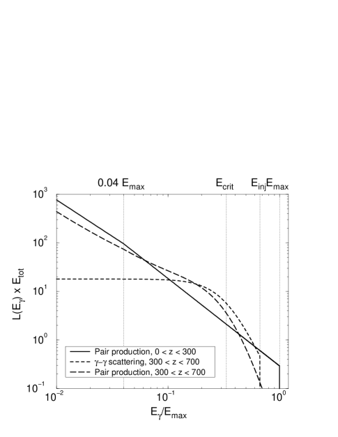
Figure 2: Scattered spectra from pair production at low $z$, photon–photon scattering, and pair production at high $z$. Each spectra has a total integrated energy of $E_{\rm tot}$, with $E_{\rm max}$ set to unity. See the text for details.

In Fig. 2 we show the spectra for pair production in the low and high $z$ regimes and the spectra for photon–photon scattering, assuming a total integrated energy of $E_{\rm tot}$ in each case. The energy is normalized with $E_{\rm max}=1$, $E_{\rm crit}=E_{\rm max}/3$ and $E_{\rm inj}=2E_{\rm max}/3$, the latter being an arbitrary choice (within the allowed range $E_{\rm max}/3<E_{\rm inj}<E_{\rm max}$) for illustration.

4 Redshifting

Given a photon spectrum after decay (from direct and/or reprocessed photons) ${\cal L}(E_{\gamma})$, the spectrum we see today is simply an integral over all redshifts convoluted with exponential decay rate,

$$\frac{dJ}{dE_{\gamma_{0}}}\;=\;\frac{3}{8\pi}\frac{t_{0}}{\tau_{\scriptscriptstyle X}}\int^{z_{0}}_{0}\frac{dz}{(1+z)^{3/2}}{\cal L}(E_{\gamma})\left(\frac{n_{\gamma}(t_{0})}{n_{\gamma}}n_{\scriptscriptstyle X}\right)\exp\left[-\frac{t_{0}}{\tau_{\scriptscriptstyle X}}(1+z)^{-3/2}\right],$$ (10)

where $\frac{dJ}{dE_{\gamma_{0}}}$ is the flux of photons, $E_{\gamma_{0}}$ is the present-day photon energy, $t_{0}$ is the age of the universe, $\tau_{\scriptscriptstyle X}$ is the lifetime of the relic, $n_{\gamma}(t_{0})$ is the present-day density of photons, and $n_{\gamma}$ and $n_{\scriptscriptstyle X}$ are respectively the densities of the photons and relics at decoupling (we use $\Omega=1$ from here on). From the previous section, we use $z_{0}=700$ as the upper limit in redshift since high energy photons injected above this redshift will pair produce off of matter and eventually Compton scatter thus avoiding direct detection. The photon spectrum today in (10) can be written suggestively as

$$\frac{dJ}{dE_{\gamma_{0}}}\;=\;B_{\gamma}\eta_{\scriptscriptstyle X}\left\{1.5\times 10^{9}\>\frac{t_{0}}{\tau_{\scriptscriptstyle X}}\int^{700}_{0}\frac{dz}{(1+z)^{3/2}}\frac{{\cal L}(E_{\gamma})}{B_{\gamma}}\exp\left[-\frac{t_{0}}{\tau_{\scriptscriptstyle X}}(1+z)^{-3/2}\right]\right\}\quad({\rm cm}^{2}{\rm~{}s~{}sr~{}MeV})^{-1},$$ (11)

where ${\cal L}(E_{\gamma})$ is in [GeV]^-1. It is clear from (11) that an upper limit on the present-day flux of photons can be translated into an upper limit on ‘the ratio of relic to photon number density’ $\eta_{\scriptscriptstyle X}$ (times the relic branching ratio to photons $B_{\gamma}$) at $z=700$.

If the lifetime is short relative to the age of the universe, then most of the photons would be reprocessed at or before recombination, and would not reach the detector. Thus, to ensure that an appreciable number of photons can be observed today, we require

$$\tau_{\scriptscriptstyle X}/t_{0}\mathrel{\>{\hbox{\raise 1.50696pt\hbox{$>$}}\kern-3.8889pt\kern-3.8889pt\hbox{\lower 2.79857pt\hbox{$\sim$}}}\>}(1+z_{0})^{-3/2}\approx 5\times 10^{-5}.$$ (12)

Furthermore, we have specified that the bound we obtain is the relic density at $z_{0}$. This is roughly equivalent to the relic density at decoupling if the lifetime is longer than (12), so that the density does not change appreciably between decoupling and $z_{0}$.

5 Diffuse Photon Background

To establish bounds on the relic density, we use the recent bounds on the extra-galactic diffuse gamma ray background from the EGRET [11] and COMPTEL [12] instruments aboard the Compton Gamma Ray Observatory. Both instruments find that the diffuse photon flux obeys a power law

$$\frac{dJ}{dE_{\gamma_{0}}}\;=\>k\left(\frac{E_{\gamma_{0}}}{1\;{\rm MeV}}\right)^{-\alpha}\qquad({\rm cm}^{2}{\rm~{}s~{}sr~{}MeV})^{-1},$$ (13)

roughly consistent with (but more sensitive than) measurements done by the SAS-2 experiment many years ago [13]. EGRET fit to a power law for photons in its observable range $30<E_{\gamma_{0}}<10^{4}$ MeV and found $k=2.26\times 10^{-3}$ and $\alpha=2.07$. COMPTEL also found a reasonable fit with $\alpha\simeq 2.3$ (although they did not explicitly give fit parameters with errors). We take the EGRET fit to be valid down to $E_{\gamma_{0}}=30$ MeV, then we estimated a best fit power law for the COMPTEL data that is continuous through $E_{\gamma_{0}}=30$ MeV. We obtained $\alpha=2.38$ with $k=6.4\times 10^{-3}$ which fits the COMPTEL data quite well down to $E_{\gamma_{0}}=0.8$ MeV (the lowest energy reported), and also fits other data [14] below the sensitivity of COMPTEL to roughly $E_{\gamma_{0}}=0.1$ MeV. We also note here that the infamous “MeV bump” discussed in Ref. [4] has disappeared.

6 Bounds from Radiative Decays

6.1 Preamble and Previous Results

Bounds on relics with radiative decays from diffuse background measurements have been considered previously in Refs. [4, 2, 5]. Our analysis differs in several ways. Many of the bounds derived here were found using the new EGRET data which allows us to look at higher energy gamma rays. Furthermore, our analysis of the showering profiles differs from those given in [4, 5]. The authors of [4, 5] determined $E_{\rm max}$ by equating the Compton scattering cross section with that from pair production, leading to a much lower value of $E_{\rm max}$ than what was used in this paper. This lower value of $E_{\rm max}$ leads to showering at lower values of the relic mass and thus the bounds found in [4, 5] have a different mass dependence than found here. As discussed in the previous section, Compton scattering does not become important until much lower energies [9] and does not play a role in the determination of $E_{\rm max}$. We also included a more complete analysis of the spectral distortion due to photon–photon scattering than was considered in [4], though the effects on the bounds are minor.

In what follows, we assume 2-body decays $X\rightarrow\gamma\gamma$ with a branching ratio $B_{\gamma}$, giving a (non-scattered) input spectrum

$$\frac{{\cal L}(E_{\gamma})}{E_{\rm inj}}=\frac{B_{\gamma}}{E_{\rm inj}}\delta(E_{\gamma}-E_{\rm inj}),$$ (14)

where we use $E_{\rm inj}=M_{\scriptscriptstyle X}/2$ to represent the injected energy per decay, with a total energy in the input spectrum of $E_{\rm tot}=2B_{\gamma}E_{\rm inj}$ (the factor of $2$ due to two photons in the final state). The bounds we find for 2-body decays can be applied approximately for 3-body decays by setting $E_{\rm inj}=\langle E\rangle=M_{\scriptscriptstyle X}/3$. In addition, 2-body decays to single photons $X\rightarrow Y\gamma$ can be similarly constrained by scaling up the bound on $\eta_{\scriptscriptstyle X}$ by a factor of two.

6.2 No scattering

In the special case that the relic decays with no scattering (so that (14) is the input spectrum), the present-day photon spectrum can be calculated exactly from (10) yielding

$$\frac{dJ}{dE_{\gamma_{0}}}=\frac{3}{8\pi}B_{\gamma}\eta_{\scriptscriptstyle X}n_{\gamma}(t_{0})\frac{t_{0}}{\tau_{\scriptscriptstyle X}}\frac{E^{1/2}_{\gamma_{0}}}{E_{\rm inj}^{3/2}}\exp\left[-\frac{t_{0}}{\tau_{\scriptscriptstyle X}}\left(\frac{E_{\gamma_{0}}}{E_{\rm inj}}\right)^{3/2}\right],$$ (15)

for $E_{\rm inj}/(1+z_{0})<E_{\gamma_{0}}<E_{\rm inj}$. The photon flux rises proportional to $E_{\gamma_{0}}^{1/2}$ up to roughly $E_{\gamma_{0}}\approx E_{\rm inj}(\tau_{\scriptscriptstyle X}/t_{0})^{2/3}$ and then drops exponentially for higher $E_{\gamma_{0}}$ up to $E_{\rm inj}$. This can be seen in Fig. 3 where sample spectra are shown for $E_{\rm inj}=20$ GeV with relic lifetimes in the range $10^{-4}\leq\tau_{\scriptscriptstyle X}/t_{0}\leq 1$. The lower bound $E_{\gamma_{0}}=E_{\rm inj}/(1+z_{0})\simeq 28.5$ MeV is clearly visible as a cutoff in the spectrum, as is the upper bound from the photon injection energy $E_{\gamma_{0}}=E_{\rm inj}=20$ GeV. Notice that for short lifetimes $\tau_{\scriptscriptstyle X}/t_{0}\mathrel{\>{\hbox{\raise 1.50696pt\hbox{$<$}}\kern-3.8889pt\kern-3.8889pt\hbox{\lower 2.79857pt\hbox{$\sim$}}}\>}10^{-4}$, the exponential suppression completely dominates the final spectra for all $E_{\gamma_{0}}$.

6.3 Numerical results, with scattering

The sample spectra in Fig. 3 illustrate the effect of redshifting, but the more general case with scattering is what is of interest to determine relic density times branching ratio bounds. In Table 1 we list the relevant scattering mechanisms with their redshift and injected energy dependence. For a given injected photon energy, we expect a dip in the spectrum due to the transition from scattered to unscattered photons as $E_{\rm inj}$ is increased. The dip is located at

$$E_{\rm dip}\;=\;\left\{\begin{array}[]{ccl}\frac{E_{\rm inj}^{2}}{E_{\rm crit}(z=0)}&&(E_{\rm inj}<55~{}{\rm GeV})\\ \frac{E_{\rm inj}}{301}&&(55<E_{\rm inj}<122~{}{\rm GeV})\\ \frac{E_{\rm inj}^{2}}{E_{\rm max}(z=0)}&&(E_{\rm inj}>122~{}{\rm GeV})\end{array}\right.,$$ (16)

where

$$E_{\rm crit}(z=0)=\frac{m_{e}^{2}}{3\cdot 22T_{0}}\approx 17~{}{\rm TeV}$$ (17)

and

$$E_{\rm max}(z=0)=\frac{m_{e}^{2}}{30T_{0}}\approx 36~{}{\rm TeV}.$$ (18)

The dependence on $E_{\rm inj}$ comes from the fact that at larger energies it is possible to scatter at smaller redshifts. This is readily seen in the $E_{\rm inj}=25,50$ GeV figures of Fig. 4. In Table 2 we evaluate (16) for the injected energies that we have considered. The photons with energies smaller than (or to the left of) $E_{\rm dip}$ are those that were reprocessed by scattering, and thus decayed at an earlier redshift then those with energy larger than (or to the right of) $E_{\rm dip}$, that were unprocessed. As we further increase $E_{\rm inj}$, pair production turns on as seen in the $E_{\rm inj}=100$, $200$ GeV figures of Fig. 4. In these figures we see the power law behavior expected at low energies coming from those photons produced in the pair production cascade.

Notice in particular that $E_{\rm inj}=100$ GeV displays a scattered spectra that is consistent with (9), whereas the scattered spectra for $E_{\rm inj}\geq 200$ GeV is consistent with (3) (see Fig. 2). The reason for this difference is that the threshold for pair production at low $z(<300)$ is crossed once $E_{\rm inj}\geq 200$ GeV, and consequently those scattered photons dominated the final spectra. It is also important to notice the critical injected energy $E_{\rm inj}=600$ GeV corresponds to an $E_{\rm dip}=10$ GeV in Table 2. For injection energies above this value, the only detectable photons will be those which undergo photon–photon scattering.

$E_{\rm inj}$				Scattering mechanism(s)
	$<$	$23$ GeV		no scattering
$23$	$\rightarrow$	$55$ GeV		photon–photon scattering ($1+z>\frac{17~{}{\rm TeV}}{E_{\rm inj}}$)
$55$	$\rightarrow$	$71$ GeV		photon–photon scattering ($1+z>301$)
$71$	$\rightarrow$	$167$ GeV		photon–photon scattering ($301<1+z<\frac{50~{}{\rm TeV}}{E_{\rm inj}}$)
$71$	$\rightarrow$	$167$ GeV		pair production ($1+z>\frac{50~{}{\rm TeV}}{E_{\rm inj}}$)
$122$	$\rightarrow$	$167$ GeV		pair production ($\frac{36~{}{\rm TeV}}{E_{\rm inj}}<1+z<301$)
$167$	$\rightarrow$	$3.7\times 10^{4}$ GeV		pair production ($1+z>\frac{36~{}{\rm TeV}}{E_{\rm inj}}$)
	$>$	$3.7\times 10^{4}$ GeV		pair production (all $z$)

Table 1: Scattering mechanisms for different injected photon energies $E_{\rm inj}$ and redshifts $z$.

$E_{\rm inj}$ (GeV)	$E_{\rm dip}$ (GeV)
$25$	$0.037$
$50$	$0.15$
$100$	$0.33$
$200$	$1.1$
$400$	$4.4$
$600$	$10$
$800$	$17$
$1600$	$70$
$3200$	$280$
$6400$	$1100$

Table 2: The location of the dip in redshifted spectra $E_{\rm dip}$, where above (below) this value the photons originated from unscattered (scattered) injected photons (see (16)). The entry in bold $E_{\rm dip}=10$ GeV, corresponding to an injected energy $E_{\rm inj}=600$ GeV is a critical point where injected energies above this value can only be detected today through scattered photons.

In Fig. 5, we have sliced the previous photon flux vs. photon energy plots along the energy axis for a particular set of observed energies $E_{\gamma_{0}}=1$, $10$, $100$, $1\times 10^{3}$ MeV. The bound on the relic density can be found by using the observational limit on the diffuse background found in Sec. 5 for each photon energy $E_{\gamma_{0}}$, and effectively inverting the graphs in Fig. 5 to give Fig. 6. These figures demonstrate that the best bound is not a trivial function of the measured photon energy, relic mass or lifetime. For example, in the $E_{\gamma_{0}}=100$ MeV figure one finds a better bound on a $25$ GeV relic particle than for somewhat heavier relics. This is due to the fact that the unscattered photons will populate the higher energy range of the observed spectrum which is more strongly constrained. Whether or not such an inversion comes about depends upon whether the energy we are considering is larger or smaller than $E_{\rm dip}$, defined in (16). For shorter lifetimes and larger photon energies, one finds the unscattered part of the spectra is exponentially suppressed, as can be seen in the lack of a limit for $E_{\gamma_{0}}=1\times 10^{3}$ MeV and small injected energies $\mathrel{\>{\hbox{\raise 1.50696pt\hbox{$<$}}\kern-3.8889pt\kern-3.8889pt\hbox{\lower 2.79857pt\hbox{$\sim$}}}\>}50$ GeV.

Finding the maximum photon flux above background (i.e. one point on each line in each graph of Fig. 4), allows one to derive the bound on the relic density for a given mass and lifetime as shown in the upper graph of Fig. 7. Bounds for lifetimes less than $\tau_{\scriptscriptstyle X}/t_{0}\approx 10^{-5}$ become poor very quickly due to the exponential suppression. Bounds for lifetimes longer than $\tau_{\scriptscriptstyle X}/t_{0}=1$ scale by a factor $t_{0}/\tau_{\scriptscriptstyle X}$ (outside (10)) relative to the bounds at $\tau_{\scriptscriptstyle X}/t_{0}=1$. We used the observational diffuse background fit as described in Sec. 5, and thus a bound for any given mass and lifetime utilizes one (optimal) observational energy. This is shown in the lower graph of Fig. 7. For example, for $\tau_{\scriptscriptstyle X}/t_{0}\geq 1$ one can see the trend in increasing $E_{\gamma_{0}}$ is to increase the photon flux (see Fig. 4). Hence the best bound for this lifetime comes from observations of the most energetic photons. On the other hand, for $\tau_{\scriptscriptstyle X}/t_{0}=10^{-4}$ one finds the best bound for $E_{\rm inj}=25$ GeV is roughly $E_{\gamma_{0}}\approx 80$ MeV. Higher $E_{\gamma_{0}}$ simply pushes into the exponential suppression regime where no bound exists. The upper limit on $M_{\scriptscriptstyle X}\eta_{\scriptscriptstyle X}\sim 2.5\times 10^{-8}$ GeV corresponds to the critical density $\Omega_{\scriptscriptstyle X}h^{2}\sim 1$, which is the upper limit for any relic based upon the age of the universe.

The general behavior in Fig. 7 is an increasing upper bound on $M_{\scriptscriptstyle X}\eta_{\scriptscriptstyle X}$ as the injected energy is raised up to about $E_{\rm inj}=800$ GeV, and then a steady decrease thereafter for larger injected energies. The reason for this trend in the bounds for 2-body decays is due to the transition noted in Table 2 when the injected energy crosses $E_{\rm inj}=600$ GeV. As remarked above, the value $E_{\rm dip}=10$ GeV at this transition implies that for all injected energies above $600$ GeV, bounds can only be derived using the scattered photons. Since the number of photons increases as the injected energy increases in the scattering regime, the bounds are stronger as the energy is increased above $600$ GeV. This effect is further enhanced by the fact that as the mass of the relic increases showering can occur at smaller redshifts. As the injected energy is reduced below $600$ GeV, more of the non-scattered, redshifted photons appear, and so a better bound comes from lowering the injected energy. This is clear since the best bound comes from the lowest injected energy considered, $E_{\rm inj}=25$ GeV. The one special case is for $E_{\rm inj}=800$ GeV where the best bound for long lifetimes $\tau_{\scriptscriptstyle X}/t_{0}\mathrel{\>{\hbox{\raise 1.50696pt\hbox{$>$}}\kern-3.8889pt\kern-3.8889pt\hbox{\lower 2.79857pt\hbox{$\sim$}}}\>}1$ is not the highest present-day detection energy, but instead slightly less $E_{\gamma_{0}}\approx 4\times 10^{3}$ MeV. The reason the bound comes from lower energies is due the $E_{\gamma}^{-4.8}$ suppression in the scattered photons that exists for present-day energies within a factor of $E_{\rm max}/E_{\rm crit}=3$ lower than $E_{\rm dip}=17$ GeV. Since the diffuse background scales as $E_{\gamma}^{-2.07\;{\rm to}\;-2.38}$, the best bound will be determined by the point where the redshifted spectrums’ slope is equal to the slope of the diffuse background . This point is roughly given by $E_{\rm dip}/3$.

It is also interesting to note that the bounds for shorter lifetimes show scalings with the mass. This can be seen by the fact that for shorter lifetimes the bounds begin to lay on top of each other in Fig. 7. This scaling is seen to group into two lines: one line of which consists of the relics whose bounds come from scattering (i.e. $E_{\rm inj}>600$ GeV) and another line for those relics whose photons can be directly detected.

7 Bounds from Hadronic Decays

The bounds on radiative decays calculated above are strong, but it is not obvious that such decays ought to dominate the branching ratio of heavy relics. Here we establish bounds on relic particles that decay through hadronic channels. We consider 3-body decays of relics into all kinematically available quark pairs and one uncolored (assumed massless) spectator.

7.1 The photon spectrum from hadronic decays

We assume general vector–axial couplings leading to both charged and neutral current mediated decays. (CKM mixing is ignored since it is in general model dependent and can be absorbed into the couplings). We take $m_{t}=175~{}{\rm GeV}$, and so two thresholds exist with increasing mass $M_{\scriptscriptstyle X}$ of the relic: $M_{\scriptscriptstyle X}=m_{t}+m_{b}$ (for charged current mediated decays) and $M_{\scriptscriptstyle X}=2\,m_{t}$ (for neutral current mediated decays). Thus, for a given mass $M_{\scriptscriptstyle X}$, an ensemble of relic decays with final quark energy and momenta spanning the 3-body phase space can be constructed.

The quark pairs are fragmented and decayed according to the string fragmentation scheme [15] implemented in Jetset [16]. This fragmentation scheme has been well tested with collider experiment data, and the resulting photon spectrum from Jetset is discussed in Ref. [17]. In particular, the exact of shape and normalization of the photon spectrum depends on the particular final state quarks [17] but generally scales with the relic mass $M_{\scriptscriptstyle X}$, which we discuss below. Once the spectrum is calculated, the present-day photon flux can be determined from (10).

The 3-body decay allows energy to escape with the uncolored decay product. Hence, the integrated photon spectrum appearing after the hadronization and decay of the $q\overline{q}^{(^{\prime})}$ system is always less than $M_{\scriptscriptstyle X}$. Furthermore, the hadronization process does not uniquely end with neutral pions, as some energy leaks into leptons. We consider only the effects of pion decays into photons. Therefore, the fraction of energy appearing in the final state (before redshifting) is generally between about $M_{\scriptscriptstyle X}/10$ and $M_{\scriptscriptstyle X}/3$ on average. This is to be contrasted with the 2-body radiative decays, where the total photonic energy injected is equal to the mass of the relic.

7.2 Generating the photon spectrum

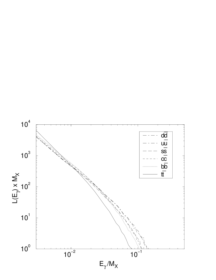
Figure 8: The photon flux from selected final state quark pairs from a 3-body decay of a relic. Notice the photon spectrum for $t\overline{t}$ has an excess of very low energy $E_{\gamma}/M_{\scriptscriptstyle X}\ll 0.01$ photons and a deficit of higher energy photons $E_{\gamma}/M_{\scriptscriptstyle X}>0.01$, compared with the photon spectra from lighter quark pairs. Note also that the spectra are effectively cutoff at $E_{\gamma}=m_{\pi}/2$, although the mass used to generate these spectra $M_{\scriptscriptstyle X}(=800\;{\rm GeV})\gg m_{\pi}$, and so the cutoff is not visible.

The photon spectrum is obtained directly from the hadronization of different final state quark pairs and is presented in Fig. 8. As we discuss below, charged current and neutral current mediated decays yield nearly identical results (except near the thresholds associated with producing one or two top quarks). As such, we will only consider neutral current decays. In total, $10^{4}$ events were generated for each final state quark pair, with each event corresponding to a point in the 3-body decay phase space. We have included final state electromagnetic and QCD radiation showers prior to fragmentation, although the showering is performed only off the final state quark pair. The particular quark pair $t\overline{t}$ is a special case since the top quark decays before it fragments. However, the photon spectrum is not particularly sensitive to Monte Carlo ordering of decay vs. fragmentation (Jetset fragments before decay). In particular, we compared the photon spectrum produced from the Pythia process $e^{+}e^{-}\rightarrow t\overline{t}$ after fragmentation (with no initial state radiation) at large energies $\sqrt{s}>2\,m_{t}$ with the top quark decaying before and after fragmentation. The photon spectrum is slightly enhanced for energies $E_{\gamma}/\sqrt{s}>0.05$ when the top quark is allowed to decay before it fragments. However, the dominant effect on our bounds from relic decays into heavy top quarks comes from the large number of photons produced at low energies. In fact, Fig. 8 clearly shows a much larger number of photons from the hadronization of light quarks ($d\overline{d}$, $u\overline{u}$, etc.) at energies $E_{\gamma}/M_{\scriptscriptstyle X}\mathrel{\>{\hbox{\raise 1.50696pt\hbox{$>$}}\kern-3.8889pt\kern-3.8889pt\hbox{\lower 2.79857pt\hbox{$\sim$}}}\>}0.01$ where one would roughly expect the slight enhancement in the top quark photon spectrum. Thus in regimes where the higher energy photons define the bound, it is the light quarks’ photon spectrum that is crucial.

The photon spectrum originates almost entirely from decaying pions, which are created in the quark fragmentation process [15, 17]. Thus, for a given decay $M_{\scriptscriptstyle X}\rightarrow q\overline{q}$, the spectra scale with $M_{\scriptscriptstyle X}$ and can be normalized to the mass of the relic. It is only the finite mass of the pion that breaks the scaling behavior. The photon spectrum is also virtually independent of the vector–axial couplings in the 3-body phase space. The only energy dependence enters in the mass of the uncolored product which we take to be negligible compared with the mass of the relic. In fact, a large non-zero uncolored product mass could be easily accommodated by simply reducing the relic mass by approximately the mass of the uncolored product.

Once the photon spectrum has been obtained from Jetset, it is fit to a sum of exponentials [17]

$${\cal L}(E_{\gamma})\times M_{\scriptscriptstyle X}\;=\;\frac{dN_{\gamma}}{dx}\;=\;A\,e^{-\alpha x}\,+\>B\,e^{-\beta x},$$ (19)

where $x\equiv E_{\gamma}/M_{\scriptscriptstyle X}$, and $A$, $B$, $\alpha$, $\beta$ are positive constants. The fit gives a reasonable characterization of the photon spectrum valid for $E_{\gamma}\mathrel{\>{\hbox{\raise 1.50696pt\hbox{$>$}}\kern-3.8889pt\kern-3.8889pt\hbox{\lower 2.79857pt\hbox{$\sim$}}}\>}m_{\pi}/2$. The dependence of the fit on the Monte Carlo statistics is small. Increasing the statistics by a factor of 5 shifts the final redshifted spectra by at most ${\cal O}(15\%)$.

7.3 Numerical results: Photon flux versus photon energy

We have scanned the relic mass range over more than two orders of magnitude from $M_{\scriptscriptstyle X}=50$ GeV (a likely lower bound from LEP) through $12.8$ TeV in steps of a factor of $2$. We have simultaneously scanned the lifetime range throughout the region that gives bounds for relevant densities. Fig. 9 displays a selection of the above sampling, with relic masses $M_{\scriptscriptstyle X}=50$, $100$, $800$, $6400$ GeV and lifetimes including $\tau_{\scriptscriptstyle X}/t_{0}=10^{-4}$, $10^{-3}$, $10^{-2}$, $10^{-1}$, $1$. The figures show the photon flux as a function of the present-day photon energy. We have also calculated the photon flux as a function of the photon energy for the same relic mass–lifetime parameter space using charged current interactions. The photon fluxes are virtually identical throughout most of the mass range, with the neutral current interaction usually giving a slightly larger value (due to decays into top quark pairs) than decays via charged current interactions. However, in the mass window $m_{t}+m_{b}<M_{\scriptscriptstyle X}<2\,m_{t}$ the photon flux from a charged current interaction is about a factor of two greater than the equivalent spectra from a neutral current interaction, since the $b\overline{t}$ decay mode is open.

It is clear from Fig. 8 that most of the photons are well below $M_{\scriptscriptstyle X}/10$, so that the effect of scattering for hadronic decays is not as prominent as in radiative decays for the same relic mass. The effects of photon–photon scattering and pair production are handled similarly to the radiative decays, however the input spectra is no longer a delta function in the photon energy. Specifically, the spectra for photon–photon scattering (6), pair production at low $z$ (3) and pair production at high $z$ (9) are used in the same way as in radiative decays. We need only determine how much energy is injected into each regime. Since the energy injected into this regime is dependent on $E_{\rm max}$ and $E_{\rm crit}$, which are in turn dependent on the redshift $z$, the procedure must be done numerically.

As noted above the non-scattered spectra are cutoff at $E_{\gamma}=m_{\pi}/2$, whereas the scattered spectra have no such cutoff. Thus, in regimes where the non-scattered (injected) spectra dominate the final redshifted spectra, we expect a cutoff at $E_{\gamma_{0}}=\frac{m_{\pi}}{2}/(1+z_{0})\approx 10^{-1}$ MeV. Such a cutoff is observed in all of the spectra in Fig. 9. Fig. 9 also shows explicit scaling with relic mass in the redshifted spectra. This is a consequence of the string fragmentation process, which is Lorentz invariant (given that enough energy is present to create a string and subsequently, jets). Scaling does not hold, however, for the scattered spectra since there are absolute cutoffs ($E_{\rm max}$, $E_{\rm crit}$) involved. Note also that despite the fact that there is no scattering, the location of the peak photon flux increases above $10^{-1}$ MeV as the lifetime is increased. This is to be expected since as the lifetime $\tau_{\scriptscriptstyle X}/t_{0}\rightarrow 1$, the peak flux should approach $m_{\pi}/2$ since photons that have not been appreciably redshifted ($z\sim 1$) are not exponentially suppressed.

Different final state quark pairs give rise to different final spectra. However, the principle differences between decays into particular final state quark pairs is not difficult to understand. As can be anticipated from the injected (non-redshifted) spectra in Fig. 8, decays into top quark pairs yield the best bound when the lowest energy photons from the injected spectra are sampled. The decay into top quark pairs gives the largest flux of photons for relics with a large mass $M_{\scriptscriptstyle X}>2m_{t}$ at very low present-day energies $E_{\gamma_{0}}\ll M_{\scriptscriptstyle X}/(1+z_{0})$. Similarly, it is the decay into light quark pairs $d\overline{d}$ and $u\overline{u}$ that give the largest flux of photons for higher energy photons $E_{\gamma_{0}}\mathrel{\>{\hbox{\raise 1.50696pt\hbox{$>$}}\kern-3.8889pt\kern-3.8889pt\hbox{\lower 2.79857pt\hbox{$\sim$}}}\>}M_{\scriptscriptstyle X}/(1+z_{0})$. Without a theoretical motivation for decays into one or another flavor or family, we choose to divide the branching ratio equally among the kinematically available quark pairs. Thus we assign an equal branching ratio for all the pairs ($1/5$ or $1/6$ depending on whether the $t\overline{t}$ threshold has been crossed).

The effect of scattering on the spectra, as remarked near the beginning of this section, is not as important for hadronic decays as it is for radiative decays. In fact, scattering is virtually absent for $M_{\scriptscriptstyle X}=50$ GeV, as illustrated in Fig. 9 where there is no photon flux (above the lower limit in the graph) for $E_{\gamma_{0}}<10^{-1}$ MeV. This is not surprising since the quark pair will always have an invariant mass less than $M_{\scriptscriptstyle X}/2$, which is only barely above the threshold for photon–photon scattering $\simeq 23$ GeV. For $M_{\scriptscriptstyle X}=100$ GeV, only photon–photon scattering is possible, and one can see the characteristic limiting behavior of a flat spectra for $E_{\gamma_{0}}<10^{-1}$ MeV. For $M_{\scriptscriptstyle X}\geq 200$ GeV, pair production dominates the scattered piece of the redshifted spectra $E_{\gamma_{0}}<10^{-1}$ MeV, albeit with a total integrated energy that is much less than the unscattered piece ($E_{\gamma_{0}}>10^{-1}$ MeV). It is really only when $M_{\scriptscriptstyle X}\mathrel{\>{\hbox{\raise 1.50696pt\hbox{$>$}}\kern-3.8889pt\kern-3.8889pt\hbox{\lower 2.79857pt\hbox{$\sim$}}}\>}1$ TeV that the scattered piece of the spectra has a photon flux comparable to the unscattered piece. This implies that the bulk of the injected photons are below about $M_{\scriptscriptstyle X}/10$, which is roughly the scale where scattering turns on.

7.4 Relic density bounds

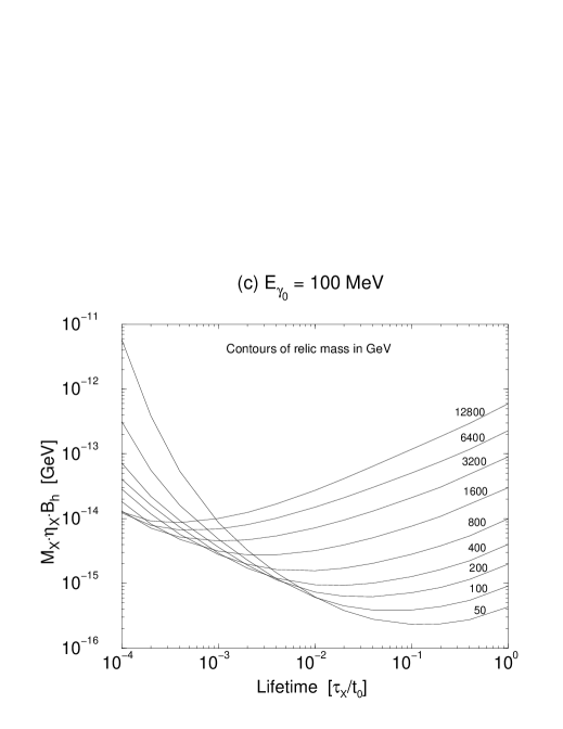
Figure 11: Upper bounds on the relic density (times the hadronic branching ratio) for particular present-day detection energies $E_{\gamma_{0}}=1$, $10$, $100$, $1\times 10^{3}$ MeV. For a given relic mass, the region with relic density larger (or above) the mass contour is excluded. Notice that better bounds do not necessarily come from higher or lower detection energies.

In Fig. 10 we have sliced the previous photon flux vs. photon energy plots along the energy axis in analogy to Fig. 5, for the particular present-day energies $E_{\gamma_{0}}=1$, $10$, $100$, $1\times 10^{3}$ MeV. Just as in the 2-body case, the bound on the relic density can be found by using the observational limit on the diffuse background found in Sec. 5 for each photon energy $E_{\gamma_{0}}$, as shown in Fig. 11. We observe, as in the 2-body radiative decays, that the mass dependence shows nontrivial behavior characteristic of the transition between relics whose bounds come the scattered and unscattered spectra respectively, for $M_{\scriptscriptstyle X}\mathrel{\>{\hbox{\raise 1.50696pt\hbox{$>$}}\kern-3.8889pt\kern-3.8889pt\hbox{\lower 2.79857pt\hbox{$\sim$}}}\>}1$ TeV. In addition, one finds that for shorter lifetimes and larger photon energies the spectra are exponentially suppressed, as can be seen in the lack of a bound for $E_{\gamma_{0}}=10^{3}$ MeV and small masses $M_{\scriptscriptstyle X}\mathrel{\>{\hbox{\raise 1.50696pt\hbox{$<$}}\kern-3.8889pt\kern-3.8889pt\hbox{\lower 2.79857pt\hbox{$\sim$}}}\>}100$ GeV. The physical interpretation is that most of the decays occurred much earlier than our present epoch, so the photon flux is significantly more redshifted than for relics with a longer lifetime. Thus, we see a much smaller number of present-day photons at high energy.

By finding the maximum photon flux above background (i.e. one point on each line in each graph of Fig. 9), one can derive the bound on the relic density for a given mass lifetime as is done in Fig. 12 (the same procedure as in Fig. 7). We used the observational diffuse background fit as described in Sec. 5, and thus a bound for any given mass and lifetime utilizes one (optimal) observational energy, as is shown in the lower graph of Fig. 12. For example, for $\tau_{\scriptscriptstyle X}/t_{0}=1$ one can see the trend in increasing $E_{\gamma_{0}}$ is to increase the photon flux (see Fig. 9). Hence the best bound for this lifetime comes from observations of the most energetic photons. On the other hand, for $\tau_{\scriptscriptstyle X}/t_{0}=10^{-4}$, one finds that the best bound for $M_{\scriptscriptstyle X}=50$ GeV is roughly $E_{\gamma_{0}}\approx 7$ MeV.

8 Implications of the Bounds

There are two central results we can extract from Figs. 7 and 12 for both radiative and hadronic decays. First, a large range of lifetimes can be excluded for a relic with roughly the critical density. Second, relics with densities considerably below the critical density are excluded, which places a strong constraint on models with a long lived massive particle.

8.1 Relics with the critical density

For relics with roughly the critical density that decay dominantly through a radiative channel, the bounds from the diffuse background exclude lifetimes in the range

$$10^{12}\mathrel{\>{\hbox{\raise 1.50696pt\hbox{$<$}}\kern-3.8889pt\kern-3.8889pt\hbox{\lower 2.79857pt\hbox{$\sim$}}}\>}\tau_{\scriptscriptstyle X}\mathrel{\>{\hbox{\raise 1.50696pt\hbox{$<$}}\kern-3.8889pt\kern-3.8889pt\hbox{\lower 2.79857pt\hbox{$\sim$}}}\>}3\times 10^{22}\;\>{\rm s}$$ (20)

(using $t_{0}=10^{10}$ yr). This bound applies to a relic with any mass $M_{\scriptscriptstyle X}\mathrel{\>{\hbox{\raise 1.50696pt\hbox{$>$}}\kern-3.8889pt\kern-3.8889pt\hbox{\lower 2.79857pt\hbox{$\sim$}}}\>}1$ MeV. The upper bound on the excluded lifetime of $3\times 10^{22}$ s applies to the worst-case scenario with $M_{\scriptscriptstyle X}/2=E_{\rm inj}\approx 600$ GeV, where the upper bound increases to roughly $10^{27}$ s for $M_{\scriptscriptstyle X}/2=E_{\rm inj}=25$ GeV and to roughly $10^{25}$ s for $M_{\scriptscriptstyle X}/2=E_{\rm inj}=6400$ GeV. The upper bounds increase for larger mass relics $M_{\scriptscriptstyle X}\mathrel{\>{\hbox{\raise 1.50696pt\hbox{$>$}}\kern-3.8889pt\kern-3.8889pt\hbox{\lower 2.79857pt\hbox{$\sim$}}}\>}10$ TeV. The upper bound on the excluded range is near $10^{28}$ s for small masses ${\cal O}(1\;{\rm GeV})$.

For relics with roughly the critical density that decay dominantly through hadronic channels, the bounds from the diffuse background exclude lifetimes in the range

$$10^{12}\mathrel{\>{\hbox{\raise 1.50696pt\hbox{$<$}}\kern-3.8889pt\kern-3.8889pt\hbox{\lower 2.79857pt\hbox{$\sim$}}}\>}\tau_{\scriptscriptstyle X}\mathrel{\>{\hbox{\raise 1.50696pt\hbox{$<$}}\kern-3.8889pt\kern-3.8889pt\hbox{\lower 2.79857pt\hbox{$\sim$}}}\>}10^{26}\;\>{\rm s}$$ (21)

for masses $M_{\scriptscriptstyle X}=50\rightarrow 10000$ GeV. Unlike 2-body decays, the upper bound on the lifetime decreases as the mass of the relic is increased. This is because for masses beyond $10$ TeV, an increasing fraction of the photons are scattered into lower energies where the diffuse photon bound is weaker. For masses smaller than $50$ GeV the upper bound on the lifetime is roughly similar, but is absent once the mass is below the threshold for pion production.

8.2 General bounds

We have shown that a large range in relic lifetime can be excluded assuming the relic has roughly the critical density. However, Figs. 7 and 12 clearly show that the upper limit on the relic density is much smaller that the critical density by several orders of magnitude. In particular, models with a long lived particle that does not have the critical density will be excluded if the relic density exceeds our bounds. The translation of our bounds is relatively straightforward, if most of the relics have not decayed prior to the earliest redshift which we considered, $z_{0}=700$ (that is, if the lifetime is longer than that in (12)). Specifically,

$$\Omega_{\scriptscriptstyle X}h^{2}\sim\frac{M_{\scriptscriptstyle X}\eta_{\scriptscriptstyle X}}{2.5\times 10^{-8}\;{\rm GeV}}$$ (22)

for $\tau_{\scriptscriptstyle X}/t_{0}\mathrel{\>{\hbox{\raise 1.50696pt\hbox{$>$}}\kern-3.8889pt\kern-3.8889pt\hbox{\lower 2.79857pt\hbox{$\sim$}}}\>}10^{-4}$.

9 Conclusions

Utilizing the latest observations of the diffuse photon background found from EGRET and COMPTEL leads to the bounds summarized in Figs. 7 and 12. Since the diffuse photon background is now well measured (up to $10$ GeV), these bounds establish a fixed upper limit on the relic density of long lived relics. We find that 3-body hadronic decays typically give better bounds than 2-body radiative decays for the same relic mass despite a larger total energy deposited into the final spectra for the latter decay mode. The stronger bounds on hadronic decays are a direct result of the low energy photons emitted from the fragmentation process that produces pions which then decay into two photons. However, strong limits on radiative decays have also been obtained for heavy mass relics since high energy photons are typically scattered by either photon–photon scattering or pair production. In particular, relics with the critical density and the masses considered here that decay dominantly through radiative (hadronic) channels are excluded for lifetimes in the range $10^{12}\mathrel{\>{\hbox{\raise 1.50696pt\hbox{$<$}}\kern-3.8889pt\kern-3.8889pt\hbox{\lower 2.79857pt\hbox{$\sim$}}}\>}\tau_{\scriptscriptstyle X}\mathrel{\>{\hbox{\raise 1.50696pt\hbox{$<$}}\kern-3.8889pt\kern-3.8889pt\hbox{\lower 2.79857pt\hbox{$\sim$}}}\>}10^{22}(10^{26})$ s. The upper bound on the excluded lifetime assumes the worst-case, which is not necessarily the smallest or largest mass. For particular masses or lifetimes, considerably more stringent bounds on the relic density can be read off from Figs. 7, 12.

The existence of strong bounds for both radiative and hadronic decays from the diffuse photon background provides a useful tool for those who consider long lived relics in particular particle physics or cosmological models. If we assume that the relic has roughly the critical density, then we have seen that the lifetime must be far greater than the age of the universe.

The bounds derived here allow for a more general analysis in that we do not make any assumptions about the number density of the relic. Thus, whether or not the relic is the dark matter, one is still able to put strong constraints on the model. Furthermore, it may be the case that the model under consideration has more than one (meta-)stable relic, one of which is a dark matter candidate. Such scenarios may arise in cases where there exist symmetries which are only broken by higher dimensional operators. For instance, in many supersymmetric models it is assumed that R parity is classically conserved. In such cases one may expect that this symmetry will be broken by gravitational effects leading to very long lived particles which may or may not be dark matter candidates. Bounds in such scenarios were discussed in Ref. [18] using limits from the positron flux in our galaxy for the case of critical density. These bounds are useful for limiting the values of the couplings involved in the decay, which in general are uncorrelated to all couplings that can be measured in accelerator experiments. However, if we do not make any assumptions regarding the energy density of the relic then we may constrain couplings that are accessible in collider experiments via a calculation of the relic density. The relic density may be determined by calculating the annihilation cross section which will be a function of the accessible parameters of the theory. The drawback to this scenario is that one must make some assumption about what is considered to be unnaturally small for the symmetry breaking couplings.

Figure 1: Dominant scattering mechanisms for high energy photons injected in the post-recombination era. The region below the solid line has an optical depth $\tau<1$, thus no scattering occurs. The other regions are dominated by $e^{+}e^{-}$ pair production (PP), photon–photon scattering (GG), pair production in matter (PPM1) and pair production in ionized matter (PPM2).

Figure 3: Photon flux as a function of photon energy ($z=0$) from a non-scattered 2-body decay (see (14)) with $M_{\scriptscriptstyle X}/2=E_{\rm inj}=20$ GeV. The spectra scale linearly with the radiative branching ratio $B_{\gamma}$ and the relic density $\eta_{\scriptscriptstyle X}$, thus an observational limit on the photon flux can be translated into a limit on $B_{\gamma}\eta_{\scriptscriptstyle X}$. A sample of relic lifetimes $\tau_{\scriptscriptstyle X}/t_{0}$ were chosen and plotted as separate contours on the graph.

Figure 4: Redshifted photon spectra for a relic with mass $M_{\scriptscriptstyle X}/2=E_{\rm inj}=25$, $50$, $100$, $200$ GeV, a 2-body decay $X\rightarrow\gamma\gamma$ with branching ratio $B_{\gamma}$, and a relic density $\eta_{\scriptscriptstyle X}$. A sample of relic lifetimes $\tau_{\scriptscriptstyle X}/t_{0}$ were chosen and plotted as separate contours on the graph.

Figure 5: Slices of Fig. 4 with present-day detection energies $E_{\gamma_{0}}=1$, $10$, $100$, $1\times 10^{3}$ MeV. To focus on the behavior of the photon flux for different masses and present-day photon detection energies, we restricted the lifetime $\tau_{\scriptscriptstyle X}/t_{0}$ to be in the range $10^{-4}\rightarrow 1$.

Figure 6: Upper bounds on the relic density (times the radiative branching ratio) for particular present-day detection energies $E_{\gamma_{0}}=1$, $10$, $100$, $1\times 10^{3}$ MeV. For a given relic mass, the region with relic density larger (or above) the mass contour is excluded. Notice that better bounds do not necessarily come from higher or lower detection energies.

Figure 7: The upper graph shows the final relic density bound for 2-body radiative decays with lifetimes in the indicated range. The bound scales linearly with the radiative branching fraction of the relic $B_{\gamma}$, although a branching ratio different from one does not strongly affect our bounds. The upper limit on the relic density of $\sim 2\times 10^{-8}$ GeV is roughly the critical density corresponding to $\Omega_{\scriptscriptstyle X}h^{2}\sim 1$. The lower graph shows the optimal photon detection energy to obtain the best bound for a given lifetime. This graph is divided at $E_{\gamma_{0}}=30$ MeV with a dotted line to show which instrument provides the diffuse photon background bound for a given lifetime.

Figure 9: Redshifted photon spectra for a relic with mass $M_{\scriptscriptstyle X}=50$, $100$, $800$, $6400$ GeV, a hadronic branching ratio $B_{h}$, and a relic density $\eta_{\scriptscriptstyle X}$. All kinematically allowed 3-body hadronic decays $X\rightarrow q\overline{q}$ ($+$ uncolored product) are assumed to occur with equal branching ratio. A sample of relic lifetimes $\tau_{\scriptscriptstyle X}/t_{0}$ were chosen and plotted as separate contours on the graph.

Figure 10: Slices of Fig. 9 with present-day detection energies $E_{\gamma_{0}}=1$, $10$, $100$, $1\times 10^{3}$ MeV. To focus on the behavior of the photon flux for different masses and present-day photon detection energies, we restricted the lifetime $\tau_{\scriptscriptstyle X}/t_{0}$ to be in the range $10^{-4}\rightarrow 1$.

Figure 12: The upper graph shows the final relic density bound for 3-body hadronic decays with lifetimes in the indicated range. The bound scales linearly with the hadronic branching fraction of the relic $B_{h}$, although a branching ratio different from one does not strongly affect our bounds. The upper limit on the relic density of $\sim 2\times 10^{-8}$ GeV is roughly the critical density corresponding to $\Omega_{\scriptscriptstyle X}h^{2}\sim 1$. The lower graph shows the optimal photon detection energy to obtain the best bound for a given lifetime. This graph is divided at $E_{\gamma_{0}}=30$ MeV with a dotted line to show which instrument provides the diffuse photon background bound for a given lifetime.

References

- [1] R. Barbieri and V. Berezinsky, Phys. Lett. B 205, 559 (1988).
- [2] S. Dodelson, Phys. Rev. D40, 3252 (1989).
- [3] V. Berezinsky, A. Masiero, and J. W. F. Valle, Phys. Lett. B 266, 382 (1991).
- [4] J. Ellis, G. B. Gelmini, J. L. Lopez, D. V. Nanopoulos, and S. Sarkar, Nucl. Phys. B373, 399 (1992).
- [5] P. Gondolo, Phys. Lett. B 295, 104 (1992).
- [6] A. A. Zdziarski and R. Svensson, Astrophys. J. 344, 551 (1989).
- [7] D. Lindley, Astrophys. J. 294, 1 (1985); M. H. Reno and D. Seckel, Phys. Rev. D37, 3441 (1988); S. Dimopoulos et al., Astrophys. J. 330, 545 (1988).
- [8] R. J. Protheroe, T. Stanev, and V. S. Berezinsky, Phys. Rev. D51, 4134 (1995).
- [9] R. Svensson and A. A. Zdziarski, Astrophys. J. 349, 415 (1990).
- [10] V. S. Berezinskii et al., “Astrophysics of Cosmic Rays”, (North-Holland, Amsterdam, 1990).
- [11] D. A. Kniffen, et al. “EGRET Observations of the High Latitude Diffuse Radiation”, 1996 (A & A in press); C. E. Fichtel, “EGRET overview: achievements in the light of expectations”, Compton Symposium, Munich, Germany, 1995.
-
[12]
S. C. Kappadath et al., “The Preliminary Cosmic Diffuse
-Ray Spectrum from 800 keV to 30 MeV Measured with COMPTEL”,
ftp://unhgro.unh.edu/pub/papers/kappadath_cdg_24icrc.ps.gz. - [13] C. E. Fichtel et al., Astrophys. J. 198, 163 (1975); C. E. Fichtel et al., Astrophys. J. 217, L9 (1977); C. E. Fichtel, G. A. Simpson, and D. J. Thompson, Astrophys. J. 222, 833 (1978).
- [14] See Fig. 2 of Ref. [12] that displays data reported in E. P. Mazets et. al., Astrophysics and Space Science, 33, 347 (1975); J. I. Trombka et. al., Astrophys. J. 212, 925 (1977).
- [15] B. Andersson, G. Gustafson, G. Ingelman, and T. Sjöstrand, Phys. Rept. 97, 31 (1983).
- [16] T. Sjöstrand, Computer Physics Commun. 82, 74 (1994).
- [17] H.-U. Bengtsson, P. Salati, and J. Silk, Nucl. Phys. B346, 129 (1990).
- [18] V. Berezinsky, A. S. Joshipura, and J. W. F. Valle, hep-ph/9608307.
- [19] I. Z. Rothstein, K. S. Babu, and D. Seckel, Nucl. Phys. B403, 725 (1993); E. Kh. Akhmedov, Z. G. Berezhiani, R. N. Mohapatra, and G. Senjanović, Phys. Lett. B 299, 90 (1993).