TOWARDS AUTOMATIC ANALYTIC EVALUATION

OF MASSIVE FEYNMAN DIAGRAMS.

L. Avdeev ,  J. Fleischer ,  M. Yu. Kalmykov   and M. Tentyukov

Fakultät für Physik, Universität Bielefeld

D-33615 Bielefeld 1, Germany

A method to calculate two-loop self-energy diagrams of the Standard Model is demonstrated. A direct physical application is the calculation of the two-loop electroweak contribution to the anomalous magnetic moment of the muon ${\frac{1}{2}(g-2)}_{\mu}$. Presently we confine ourselves to a “toy” model with only $\mu$, $\gamma$ and a scalar particle (Higgs). The algorithm is implemented as a package of computer programs in FORM. For generating and automatically evaluating any number of two-loop self-energy diagrams, a special C-program has been written. This program creates the initial FORM-expression for every diagram generated by QGRAF, executes the corresponding subroutines and sums up the final results.

Keywords: Standard Model, Feynman diagram, recurrence relations, anomalous magnetic moment

1 Introduction

Recent high precision experiments to verify the Standard Model of electroweak interactions require, on the side of the theory, high precision calculations resulting in the evaluation of higher loop diagrams. For specific processes thousands of multi-loop Feynman diagrams do contribute, and it turns out impossible to perform these calculations by hand. That makes the request for automatization a high priority task. In this direction, several program packages are elaborated (^{? ?} and reports of the Minami-Tateya collaboration, Bauberger et al., Pukhov et al., Vermaseren and J.X.Wang on this conference). It appears absolutely necessary that various groups produce their own solutions of handling this problem: the various ways will be of different efficiency, have different domains of applicability, and last but not least, should eventually allow for completely independent checks of the final results. This point of view motivated us to seek our own way for automatic evaluation of Feynman diagrams. We have in mind only higher loop calculations (no multipoint functions).

We demonstrate here the functioning of a C-program (TLAMM) for the evaluation of the two-loop anomalous magnetic moment (AMM) of the muon ${\frac{1}{2}(g-2)}_{\mu}$, but on the same lines we have developed the program to an extent that it can be applied to arbitrary processes in the Standard Model. This piloting C-program must read the diagrams generated by QGRAF ^? for a given physical process, generate the FORM ^? source code, start the FORM interpreter, read and sum up the results for the class of diagrams under consideration. For the purpose of demonstration, here we apply TLAMM to a closed subclass of diagrams of the Standard Model, which we refer to as a “toy” model.

Recent papers reduced the theoretical uncertainty of the muon AMM by partially calculating the two-loop electroweak contributions ^?, ^?. Their results have been obtained in the following approximation: terms suppressed by $(1-4\sin^{2}\Theta)$ were omitted; the fermion masses of the first two families are set to zero; in the third family the $\tau$- and $b$-quark masses are taken to be zero as well; diagrams with two or more scalar couplings to the muon are suppressed by the ratio $\frac{m^{2}_{\mu}}{M^{2}_{Z}}$ and have been discarded; the Kobayashi-Maskawa matrix is assumed to be unity; the mass of the Higgs particle is large compared to $M_{Z,W}$.

All of these approximations, except possibly the last one, are well justified and give rise to small corrections only. We consider it of great interest to study also the case $M_{H}\sim M_{Z,W}$. To perform this calculation is our main physical motivation. Apart from that, for technical reasons, it may be interesting to study the functioning of TLAMM by calculating all $1832$ two-loop diagrams without any approximation.

The calculation of the anomalous magnetic moment of the muon reduces, after differentiation and contractions with projection operators, to diagrams of propagator type with external momentum on the muon mass-shell (for details see ^?).

The method of Taylor expansion of diagrams in external momenta and Padé approximation ^? yields only slowly converging results at the threshold. Since in the case of the muon AMM we are confronted with a low energy problem it appears natural to expand with respect to the heavy masses ($M_{Z},M_{H}$ and $m_{t}$) of the theory. The applicability of the “asymptotic-R-operation” ^? in the limit of large masses has to be investigated for diagrams evaluated on the muon mass-shell(i.e. $p^{2}=-m_{\mu}^{2}$). Some diagrams already had a threshold at the muon mass-shell before the expansion. In other diagrams this threshold appears in some terms of the expansion. In dimensional regularization, threshold singularities (like any other infrared singularities if they are strong enough) manifest themselves as poles in $\varepsilon$ (d=4-2$\varepsilon$). They ought to cancel for the total AMM. We check this in our toy model.

2 Large-mass expansion

The asymptotic expansion in the limit of large masses is defined ^? as

$$F_{G}(q,M,m,\varepsilon)\stackrel{{\scriptstyle M\to\infty}}{{\sim}}\sum_{\gamma}F_{G/\gamma}(q,m,\varepsilon)\circ T_{q^{\gamma},m^{\gamma}}F_{\gamma}(q^{\gamma},M,m^{\gamma},\varepsilon)$$ (1)

where $G$ is the original graph, $\gamma$’s are subgraphs involved in the asymptotic expansion, $G/\gamma$ denotes shrinking $\gamma$ to a point; $F_{\gamma}$ is the Feynman integral corresponding to $\gamma$; $T_{q^{\gamma},m^{\gamma}}$ is the Taylor operator expanding the integrand in small masses $\{m_{\gamma}\}$ and external momenta $\{q_{\gamma}\}$ of the subgraph $\gamma$ (before integration); “$\circ$” inserts the subgraph expansion in the numerator of the integrand $F_{G/{\gamma}}$. The sum goes over all subgraphs $\gamma$ which (a) contain all lines with large masses, and (b) are one-particle irreducible relative to lines with light masses.

The following types of integrals occur in the asymptotic expansion of the muon AMM in the Standard Model: $1.$ two-loop tadpole diagrams with various heavy masses on internal lines; $2.$ two-loop self-energy diagrams, involving contributions from fermions lighter or heavier than the muon, with the external momentum on the muon mass-shell; $3.$ two-loop self-energy diagrams with two or three muon lines and the external momentum on the muon mass-shell; $4.$ products of one-loop self-energy diagrams on-shell and a one-loop tadpole with a heavy mass. Almost all of these diagrams can be evaluated analytically using the package SHELL2 ^?. For our calculation we have modified this package in the following way: $1.$ There are no restrictions on the indices on the lines (powers of scalar denominators). $2.$ More recurrence relations are used, and the dependence on the space-time dimension is always explicitly reducible to powers of linear factors. $3.$ A new algorithm for simplification of this rational fractions is implemented. These modifications essentially reduce the execution time (in some cases, down to the order of a hundredth). $4.$ New programs for evaluating two-loop tadpole integrals with different masses are added. $5.$ New programs were written for the asymptotic expansion of one-loop self-energy diagrams (relevant for renormalization) in the large-mass limit.

3 The toy-model

As the first step, we concentrate on a “toy” model, a “slice” of the Standard Model, involving a light charged spinor $\Psi$, the photon $A_{\mu}$, and a heavy neutral scalar field $\Phi$. The scalar has triple $\left(g\right)$ and quartic $\left(\lambda\right)$ self-interactions, and the Yukawa coupling to the spinor $\left(y\right)$. The Lagrangian of the toy-model reads (in the Euclidean space-time):

$${\it L} = \frac{1}{2}\partial_{\mu}\Phi\partial^{\mu}\Phi+\frac{1}{2}M^{2}\Phi^{2}-\frac{g}{3!}\Phi^{3}-\frac{\lambda}{4!}\Phi^{4}+\frac{1}{4}F_{\mu\nu}^{2}+\frac{1}{2\alpha}\left(\partial_{\mu}A^{\mu}\right)^{2}$$ (2)

$$+\bar{\Psi}\left(\hat{\partial}+m\right)\Psi+ie\bar{\Psi}\hat{A}\Psi-y\Phi\bar{\Psi}\Psi$$

where $e$ is the electric charge and $\alpha$ is a gauge fixing parameter.

The main aims of the present investigation are the following:

$1.$ Verification of the consistency of the large-mass asymptotic expansion with the external momentum on the mass shell of a small mass. In particular, we check the cancelation of all threshold singularities, that appear in individual diagrams and manifest themselves as infrared poles in $\varepsilon$.

$2.$ Estimation of the influence of a heavy neutral scalar particle on the AMM of the muon in the framework of the Standard Model.

$3.$ Verification of gauge independence: we use the covariant gauge with an arbitrary parameter $\alpha$.

In the following we analyze in some detail the diagrams contributing to the AMM of the fermion in our toy-model and specify the renormalization procedure. Apart from counterterms $40$ diagrams contribute to the two-loop AMM of the fermion. After performing the Dirac and Lorentz algebra, all diagrams can be reduced to some set of scalar prototypes. A “prototype” defines the arrangement of massive and massless lines in a diagram. Individual integrals are specified by the powers of the denominators, called indices of the lines. From the point of view of the asymptotic expansion method the topology of the diagram is essential. All diagrams of the toy-model which contribute to the two-loop AMM can be classified in terms of $9$ prototypes (we omit the pure QED diagrams). These prototypes and their corresponding subgraphs $\gamma$ involved in the asymptotic expansion, are given in Fig. 1. In dimensional regularization, the last subgraphs vanish in cases $1,4,7$, and $8$, owing to massless loops.

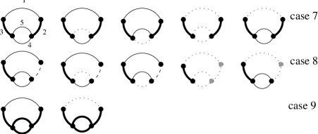
Figure 1: The prototypes and their subgraphs contributing to the large mass expansion. Bold, thin and dashed lines correspond to the heavy-mass, light-mass, and massless propagators, respectively. Dotted lines indicate the lines omitted in the subgraph $\gamma$.

All diagrams were generated in symbolic form by means of QGRAF ^?. The TLAMM-program

$1.$ Reads QGRAF output;

$2.$ For each diagram, it creates a file containing the complete FORM program for calculating this diagram;

$3.$ Executes FORM;

$4.$ Reads FORM output, picks out the result of the calculation, and builds the total sum of all diagrams in a single file.

All initial settings are defined in the “configuration file”. It contains information about the use of file names, identifiers of topologies, choice of momenta, and the description of the model in terms of the notation that is some extension of QGRAF’s. All diagrams are classified according to their prototypes. Identifiers for vertices and propagators and explicit Feynman rules are read from separate files and then inserted into the FORM program. For each diagram, the relevant FORM subroutines are called. Since the number of identifiers needed for the calculation of all diagrams may exceed FORM capacity, the TLAMM-program keeps for each diagram only those needed for its calculation. Finally, the total sum of all diagrams is put into one file and can be processed further by FORM. There exist several options which allow one to process only diagrams $1$ with given numbers; $2$ of a given prototype; $3$ of a specified topology; and some debugging options.

To perform the asymptotic expansion FORM-programs have been written for every prototype. For efficiency of the algorithm the following is essential:

$1.$ The result of the calculation is presented as a series in small parameters. Care is taken to avoid the production of unnecessary high powers in intermediate results.

$2.$ For the evaluation of the Feynman integrals it is necessary to reduce scalar products of momenta in the numerator to the square combinations present in the denominator. Most efficiently, this is done by means of recurrence relations proposed by Tarasov ^? in the proceeding of the AIHENP-$95$.

We use the on-shell renormalization scheme. The renormalization conditions are as follows: $1.$ The electric charge $e$ is defined in terms of the nonrelativistic Thompson limit of the Compton scattering. $2.$ The physical masses are given as the pole of the propagators. Since we are interested here only in the AMM, we don’t need the wave-function renormalization. All the tadpoles are canceled by mass counterterms. Then at the two-loop level the interaction $\Phi^{4}$ does not contribute to the AMM of the fermion. No special functions but the logarithms appear in the final result:

$$a_{\mu} = \frac{e^{2}}{4\pi^{2}}\left\{\frac{1}{2}\right\}+\frac{e^{4}}{16\pi^{4}}\left\{\frac{197}{144}+\left(\frac{1}{2}-3\ln\left(2\right)\right)\zeta\left(2\right)+\frac{3}{4}\zeta\left(3\right)\right\}$$ (3)

$$+\frac{y^{2}}{16\pi^{2}}\left(\frac{m}{M}\right)^{2}\left\{-\frac{7}{3}+2\ln\left(\frac{M}{m}\right)^{2}\right\}$$

$$+\frac{e^{2}y^{2}}{64\pi^{4}}\left(\frac{m}{M}\right)^{2}\left\{\frac{335}{27}+\frac{121}{9}\ln\left(\frac{M}{m}\right)^{2}-\frac{13}{2}\ln^{2}\left(\frac{M}{m}\right)^{2}-29\zeta\left(2\right)\right\}$$

$$+\frac{y^{3}}{256\pi^{4}}\left(\frac{gm}{M^{2}}\right)\left\{2-\frac{4}{3}\zeta\left(2\right)+\left(\frac{m}{M}\right)^{2}\left\{\frac{46}{3}-\frac{189}{2}S_{2}+6\ln\left(\frac{M}{m}\right)^{2}\right\}\right\}$$

$$+\frac{y^{2}}{256\pi^{4}}\left(\frac{gm}{M^{2}}\right)^{2}\left\{-\frac{5}{3}+\frac{45}{2}S_{2}-\frac{13}{3}\frac{\pi}{\sqrt{3}}-\left(2-\frac{16\pi}{\sqrt{3}}\right)\ln\left(\frac{M}{m}\right)^{2}\right\}$$

$$+\frac{y^{4}}{256\pi^{4}}\left(\frac{m}{M}\right)^{2}\left\{\frac{103}{6}-13\ln\left(\frac{M}{m}\right)^{2}\right\}$$

where $S_{2}=\frac{4}{9\sqrt{3}}{\it Cl}_{2}\left(\frac{\pi}{3}\right)=0.2604341$ with ${\it Cl}_{2}$ the Clausen function, $e^{2}/(4\pi)\equiv\frac{1}{137}$ and $y,g$ are renormalized coupling constants. We see that

$1$ The two-loop contribution to the AMM is gauge independent.

$2$ The additional threshold singularities arising in the asymptotic R-operation have canceled.

$3$ With the Standard Model values it is $\sim\left(\frac{m}{M}\right)^{4}$.

References

References

- [1] T. Ishikawa et al., Minami-Tateya group “GRACE manual”, KEK-92-19, 1993.
- [2] J. Kublbeck, M. Böhm and A. Denner, Comp. Phys. Comm. 60 (1990), 165.
- [3] P. Nogueira, J. Comput. Phys. 105 (1993), 279.
- [4] J. A. M. Vermaseren, Symbolic manipulation with FORM, Amsterdam, Computer Algebra Nederland, 1991.
- [5] T. V. Kukhto, E. A. Kuraev, A. Schiller and Z. K. Silagadze, Nucl. Phys. B371 (1992), 567; E. A. Kuraev, T. V. Kukhto, and A. Schiller, Sov. J. Nucl. Phys. 51 (1990), 1031.
- [6] A. Czarnecki, B. Krause and W. Marciano, Phys. Rev. D52 (1995), R2619; Phys. Rev. Lett. 76 (1996), 3267; Preprint TTP96-21 (hep-ph/9606393).
- [7] R. Z. Roskies, E. Remiddi and M. J. Levine in Quantum Electrodynamics, p. 163, ed. T. Kinoshita (World Scientific, Singapore, 1990).
- [8] J. Fleischer and O. V. Tarasov, Z.Phys. C64 (1994), 413; J. Fleischer, Int.J.Mod.Phys. C6 (1995), 495; J. Fleischer, V. A. Smirnov and O. V. Tarasov, Preprint Bi-TP 95/39, to be published in Z.Phys. C (hep-ph/9605392).
- [9] F. V. Tkachov, Preprint INR P-0358 (Moscow, 1984); Int. J. Mod. Phys. A8 (1993), 2047; G. B. Pivovarov and F. V. Tkachov, Preprint INR P-0370 (Moscow, 1984); Preprint INR P-0459 (Moscow, 1986); Int. J. Mod. Phys. A8 (1993), 2241; S. G. Gorishny and S. A. Larin, Nucl. Phys. B283 (1987), 452; K. G. Chetyrkin, Teor. Math. Phys. 75 (1988), 26; ibid 76 (1988), 207; Preprint MPI-PAE/PTh-13/91 (Munich, 1991); V. A. Smirnov, Comm. Math. Phys. 134 (1990), 109; Renormalization ans asymptotic expansions (Bikrhäuser, Basel, 1991).
- [10] F. A. Berends, A. I. Davydychev, V. A. Smirnov and J. B. Tausk, Nucl. Phys. B 439 (1995), 536.
- [11] J. Fleischer and O. V. Tarasov, Comp. Phys. Commun. 71 (1992), 193.
- [12] O.V. Tarasov, in New Computing Techniques in Physics Research IV, ed. B. Denby and D. Perret-Gallix (World Scientific, Singapore, 1995), p.161 (hep-ph/9505277).