Abstract

We calculate the two-loop vertex function for the crossed topology, and for arbitrary masses and external momenta. We derive a double integral representation, suitable for a numerical evaluation by a Gaussian quadrature. Real and imaginary parts of the diagram can be calculated separately.

PACS numbers: 02.70.+d, 12.38.Bx, 11.20.Dj

1 Introduction

In the recent past many efforts have been made to calculate two-loop Feynman diagrams with masses, e.g. [1, 2, 3, 4, 5]. Though now very effective methods exist for the general mass case of the two-loop two point function [6, 7], these methods need considerable extensions or modifications to cope with two-loop three-point functions in general. The planar topology has been discussed extensively, e.g. in [2, 3, 8, 9]. For the other important topology — the crossed topology — so far two methods have been presented.

The method presented in [5] is based on Feynman parameters and uses high dimensional Monte Carlo integration, resulting in extensive CPU usage and slow convergence when high accuracy is needed.

Taylor expansion, analytic continuation and Padé approximations, as presented in [4], gives results with very high accuracy, but the method is, at this stage, still restricted to one kinematical variable.

Our approach is based on [2, 3], where it gave excellent results for the planar two-loop three point function. The calculation of the crossed topology is similar to the planar case. Again we succeed by considering orthogonal and parallel space variables. From this starting point, a four-fold integration is immediately obtained. Still following the lines of [3] we use Euler transformations for subsequent integrations. The difference between the planar and the non-planar topology is apparent in the increasing number of different cases which have to be considered for the latter, while, fortunately, the conceptual frame remains unaffected. Once more we end up with a two-fold integral over a finite region, solely involving dilogarithms and related functions. This integral representation allows for a Gaussian quadrature, and is thus perfectly suitable for practical purposes [10].

2 Calculation

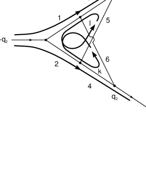
Figure 1: The two-loop crossed vertex function.

Our task is to calculate the two-loop crossed vertex function, as shown in fig.1. We restrict ourselves to the scalar integral, which is given by

$$V(q_{1},q_{2})=\int\!\!d^{4}l\int\!\!d^{4}k\frac{1}{P_{1}P_{2}P_{3}P_{4}P_{5}P_{6}}\,,$$ (1)

where $q=q_{1}+q_{2}$ is the momentum of the incoming particle and $q_{1}$ and $q_{2}$ are the momenta of the outgoing particles. Further, $l$ and $k$ are the internal loop momenta, and $P_{i}$, $i=1\dots 6$ are the propagators of the internal particles, as labeled in fig.1. We assume that all external particles are massive and have time-like momenta. The massless limit is approached smoothly as long as no on-shell singularities occur.

The integral will be splitted into parallel and orthogonal space integrations. The parallel space is two-dimensional here, hence leaving two dimensions for the orthogonal space. The integral is convergent in $D=4$ dimensions, and there is no need to use a regularization scheme.

Since the integral is Lorentz invariant, the splitting into parallel and orthogonal space variables is equivalent to the choice of a Lorentz frame. For time-like external particles, we choose the rest frame of the incoming particle, and assume that outgoing particles are moving along the $x$-axis.

Explicitly, the four-momenta are chosen as

$$q^{\mu} = (e_{1}+e_{2},0,0,0)$$

$$q_{1}^{\mu} = (e_{1},q_{z},0,0)$$

$$q_{2}^{\mu} = (e_{2},-q_{z},0,0)$$

$$l^{\mu} = (l_{0},l_{1},\vec{l}_{\perp})$$

$$k^{\mu} = (k_{0},k_{1},\vec{k}_{\perp})$$ (2)

with $q_{z}$, $e_{1}$ and $e_{2}$ positive and $q_{z}<e_{1}$, $q_{z}<e_{2}$.

The propagators $P_{i}$ of the internal particles can be written down using the flow of loop momenta as shown in fig.1

$$P_{1} = (l+k-q_{1})^{2}-m_{1}^{2}+i\eta$$

$$P_{2} = (l+k+q_{2})^{2}-m_{2}^{2}+i\eta$$

$$P_{3} = (l-q_{1})^{2}-m_{3}^{2}+i\eta$$

$$P_{4} = (k+q_{2})^{2}-m_{4}^{2}+i\eta$$

$$P_{5} = l^{2}-m_{5}^{2}+i\eta$$

$$P_{6} = k^{2}-m_{6}^{2}+i\eta\,.$$ (3)

A small imaginary part $-i\eta$ with $\eta>0$ is assigned to the squared masses of the internal particles and is chosen equal for all particles for convenience. Hence differences of propagators have a vanishing imaginary part, which we utilize in the following. The choice of different (small, positive) $\eta_{i}$’s for the propagator would not change our final result, but is technically more cumbersome.

Using the explicit representation of the momenta in eq.(2), a shift of the loop momenta with a trivial Jacobian according to

$$l_{1} \rightarrow l_{1}+q_{z}$$

$$l_{0} \rightarrow l_{0}+l_{1}$$

$$k_{0} \rightarrow k_{0}+k_{1}\,,$$ (4)

achieves that the propagators are linear in $l_{1}$ and $k_{1}$ and hence can be written as

$$P_{1} = (l_{0}+k_{0}-e_{1})^{2}+2(l_{0}+k_{0}-e_{1})(l_{1}+k_{1})-l_{\perp}^{2}-k_{\perp}^{2}-2l_{\perp}k_{\perp}z-m_{1}^{2}+i\eta$$

$$P_{2} = (l_{0}+k_{0}+e_{2})^{2}+2(l_{0}+k_{0}+e_{2})(l_{1}+k_{1})-l_{\perp}^{2}-k_{\perp}^{2}-2l_{\perp}k_{\perp}z-m_{2}^{2}+i\eta$$

$$P_{3} = (l_{0}-e_{1})^{2}+2(l_{0}-e_{1})l_{1}-l_{\perp}^{2}-m_{3}^{2}+i\eta$$

$$P_{4} = (k_{0}+e_{2}+q_{z})^{2}+2(k_{0}+e_{2}+q_{z})(k_{1}-q_{z})-k_{\perp}^{2}-m_{4}^{2}+i\eta$$

$$P_{5} = (l_{0}-q_{z})^{2}+2(l_{0}-q_{z})(l_{1}+q_{z})-l_{\perp}^{2}-m_{5}^{2}+i\eta$$

$$P_{6} = k_{0}^{2}+2k_{0}k_{1}-k_{\perp}^{2}-m_{6}^{2}+i\eta\,,$$ (5)

where $z$ is the cosine of the angle between $\vec{l}_{\perp}$ and $\vec{k}_{\perp}$.

The volume element in the integral in eq.(1) is given by (cf. [3])

$$d^{4}l\,d^{4}k=\frac{1}{2}dl_{0}\,dk_{0}\,dl_{1}\,dk_{1}\,ds\,dt\,d\alpha\,\frac{dz}{\sqrt{1-z^{2}}}$$ (6)

with $s\equiv l_{\perp}^{2}$, $t\equiv k_{\perp}^{2}$ and the angle $\alpha$ describing the absolute position of $\vec{l}_{\perp}$ and $\vec{k}_{\perp}$. The integration over $\alpha$ gives a trivial factor $2\pi$.

An important difference between the crossed and the planar two-loop vertex function is that now necessarily two (instead of one) propagators depend on $z$, which, in our notation, are $P_{1}$ and $P_{2}$. This is a result of the fact that in the planar case the loop momenta can be arranged to flow through only one common propagator, which is not possible for the crossed topology.

But after applying a partial fraction decomposition to the integrand

$$\frac{1}{P_{1}P_{2}P_{3}P_{4}P_{5}P_{6}}=\frac{1}{(P_{2}-P_{1})P_{1}P_{3}P_{4}P_{5}P_{6}}+\frac{1}{(P_{1}-P_{2})P_{2}P_{3}P_{4}P_{5}P_{6}}$$ (7)

the $z$-dependence in $P_{1}-P_{2}$ drops out and the $z$-integration can be performed as in the planar case:

$$\int\limits_{-1}^{1}\frac{dz}{\sqrt{1-z^{2}}}\frac{1}{A_{k}+B_{k}z+i\eta}=\frac{\pi}{\sqrt[c]{A_{k}^{2}-B_{k}^{2}+2A_{k}i\eta}},\quad k=1,2$$ (8)

where $P_{1}=A_{1}+B_{1}z+i\eta$ for the first term in eq. (7) and $P_{2}=A_{2}+B_{2}z+i\eta$ in the second, respectively. $\sqrt[c]{z}$ denotes the square root of a complex number with a cut along the positive real axis, whereas $\sqrt{x}$ is the usual square root of a positive real number (if $x$ has a small imaginary part of any sign, it can be ignored).

The next step is the integration over $l_{1}$ and $k_{1}$ using Cauchy’s theorem for both of them. It is important to notice that, as a result of the partial fraction decomposition in eq. (7), in the difference $P_{1}-P_{2}$ the imaginary part of the masses $-i\eta$, which has been chosen to be equal for all masses, drops out. Therefore not all poles in $l_{1}$ and $k_{1}$ lie in the upper or lower complex half-plane, but some also on the real axis. The integral can be made meaningful if interpreted as a principal value integral. Then one has to use the modified Cauchy’s theorem [11]:

$${\mbox{P$\!$.V$\!$.}}\!\int\limits_{-\infty}^{\infty}f(z)\,dz = 2i\pi\sum_{i}^{n}\mbox{Res}(f(z))\bigg{|}_{z=z_{i},\,\mbox{\scriptsize Im}(z_{i})\!\!\begin{array}[]{c}\mbox{\tiny$<$}\\[-6.32918pt] \mbox{\tiny$>$}\end{array}\!\!0}$$ (12)

$$+i\pi\sum_{j}^{m}\mbox{Res}(f(z))\bigg{|}_{z=z_{j},\,\mbox{\scriptsize Im}(z_{j})=0},$$

where the $z_{i}$ are the $n$ poles of $f(z)$ inside the closed integration contour, whereas $z_{j}$ are $m$ poles along the integration path. Poles on the path contribute only with half the weight compared to poles inside the path. For the cases we are confronted with it is guaranteed that the function tends to zero sufficiently fast for large $l_{1}$ and $k_{1}$, hence the theorem is applicable.

The integration path has to be closed either in the upper or in the lower complex half-plane, depending on the position of the cuts of the square root $\sqrt[c]{A^{2}-B^{2}+2Ai\eta}$. Similarly to the planar case, the position of the cuts is determined by the sign of $l_{0}+k_{0}-e_{1}$ for the first term in eq.(7) and by the sign of $l_{0}+k_{0}+e_{2}$ for the second term.

Let us concentrate on the first term of the partial fraction decomposition, the second can be handled analogously. Assume $l_{0}+k_{0}-e_{1}<0$, so that we have to close the contour of the $l_{1}$ integration in the lower half-plane. Then, some propagators have poles inside the path: $P_{3}$ iff $l_{0}-e_{1}>0$ and $P_{5}$ iff $l_{0}-q_{z}>0$. Additionally, $P_{2}-P_{1}$ always contributes with half its residue, since it has a pole on the real axis. In the following we will call residues, which involve only $P_{3}\dots P_{6}$, complex contributions, because all poles lie in the upper or lower complex half-plane, whereas residues involving $P_{1}-P_{2}$ are called real contributions, because the pole lies on the real axis.

For the $k_{1}$ integration, we close the contour in the same half-plane as for the $l_{1}$ integration, depending on the sign of $l_{0}+k_{0}-e_{1}$. This is not necessary for the $P_{2}-P_{1}$ contribution, where the square root becomes independent of $k_{1}$, but it is done for consistency. Let us first assume that we had a $l_{1}$-pole in $P_{3}$. Then we have poles in $k_{1}$ from $P_{4}$ iff $k_{0}+e_{2}+q_{z}>0$ and $P_{6}$ iff $k_{0}>0$, and a pole in $P_{2}-P_{1}$, iff $l_{0}-e_{1}<0$. But the last case is a contradiction to $l_{0}-e_{1}>0$ above, so it does not contribute.

Analogously, if we had a $l_{1}$-pole in $P_{5}$, we have the same constraints from $P_{4}$ and $P_{6}$, but $l_{0}-q_{z}<0$ from $P_{2}-P_{1}$, which is again a contradiction.

The last case, a $l_{1}$-pole in $P_{2}-P_{1}$, gives contributions from all other propagators, namely $P_{3}$ iff $l_{0}-e_{1}<0$, $P_{4}$ iff $k_{0}+e_{2}+q_{z}>0$, $P_{5}$ iff $l_{0}-q_{z}<0$ and $P_{6}$ iff $k_{0}>0$.

If $l_{0}+k_{0}-e_{1}>0$, the relation operators have to be reversed in all inequalities. Out of the complex combinations, only the pairs $(P_{3},P_{4})$, $(P_{5},P_{4})$ and $(P_{5},P_{6})$ contribute in triangular regions in the $(k_{0},l_{0})$ plane if $l_{0}+k_{0}-e_{1}<0$ (see fig.2). If $l_{0}+k_{0}-e_{1}>0$, no terms contribute. All real residues contribute for $l_{0}+k_{0}-e_{1}<0$ as well as for $l_{0}+k_{0}-e_{1}>0$. The areas are not triangles, but unbound, as can be seen in fig.3.

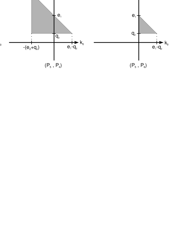
Figure 2: Triangles from the first term of the partial fraction decomposition (complex contributions).

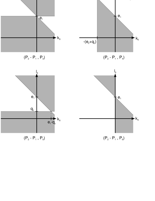
Figure 3: Unbound areas from the first term of the partial fraction decomposition (real contributions).

The second term of the partial fraction decomposition also gives us three contributing complex residues (all for $l_{0}+k_{0}+e_{2}>0$, fig.4) and four real residues, which have the same constraints as for the first term, but with $l_{0}+k_{0}-e_{1}\begin{array}[]{c}<\\[-7.3194pt] >\end{array}0$ replaced by $l_{0}+k_{0}+e_{2}\begin{array}[]{c}<\\[-7.3194pt] >\end{array}0$ (fig.5).

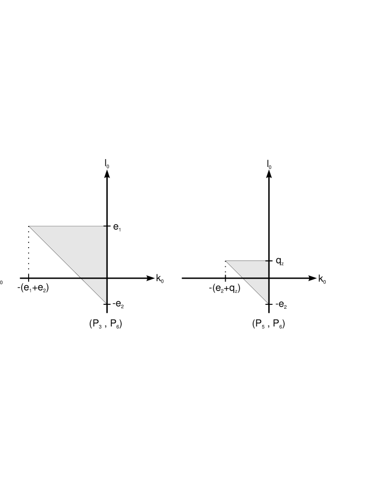
Figure 4: Triangles from the second term of the partial fraction decomposition (complex contributions).

Figure 5: Unbound areas from the second term of the partial fraction decomposition (real contributions).

If we compare the real contributions from both terms of the partial fraction decomposition eq.(7), we notice that the terms for two corresponding residues (e.g. $(P_{2}-P_{1},P_{3})$ and $(P_{1}-P_{2},P_{3})$) are equal, except for an overall minus sign. As a consequence they cancel in the area where both contribute together. This is everywhere the case except in the strip $-e_{2}<l_{0}+k_{0}<e_{1}$ (see fig.6). Furthermore it can be shown that all four real contributions from fig.6 add up to zero where they all contribute together. This is the case everywhere outside the finite area shown in fig.7, which is also the joined area of all triangles in figs.2 and 4 from the complex residues.

Figure 6: Sum of both terms of the pfd for the real contributions (dark shading from the first, light shading from the second term $=$ $-$ first term.)

Figure 7: Sum of all four terms from fig. 6.

After the residue integrations we end up with a four-fold integral representation which is similar in nature, but slightly more complicated in its technical appearance than the planar case. It can be written in the general form

$$V(q_{1},q_{2}) = \sum_{j}\int\!\!\!\!\int\limits_{A_{j}}\!\!dl_{0}\,dk_{0}\int\limits_{0}^{\infty}\!\!ds\int\limits_{0}^{\infty}\!\!dt\>C(k_{0},l_{0})$$ (13)

$$\frac{1}{\tilde{a}_{1}t+\tilde{b}_{1}+\tilde{c}_{1}s}\frac{1}{\tilde{a}_{2}t+\tilde{b}_{2}+\tilde{c}_{2}s}\frac{1}{\tilde{a}_{3}t+\tilde{b}_{3}+\tilde{c}_{3}s}\frac{1}{\sqrt[c]{(at+b+cs)^{2}-4st}}\,.$$

The $j$-sum runs over all areas $A_{j}$ depicted in figs.2 – 5. The coefficients $C(k_{0},l_{0})$, $\tilde{a}_{i}$, $\tilde{b}_{i}$, $\tilde{c}_{i}$ ($i=1\dots 3$), $a$, $b$ and $c$ are in general dependent on $j$, $l_{0}$ and $k_{0}$. $\tilde{b}_{i}$ and $b$ have an infinitesimal imaginary part, all other coefficients are real. Some coefficients are vanishing: for the complex residues, $\tilde{a}_{1}$ and $\tilde{c}_{3}$ are zero, and we have one pure pole in $s$, one in $t$ and a mixed $(s,t)$ pole. For the real residues, either $\tilde{c}_{3}=0$ or $\tilde{a}_{3}=0$, i.e. we have two mixed poles and either one pure pole in $t$ or in $s$. In the latter case we can relabel $s{\displaystyle\leftrightarrow}t$, together with exchanging $\tilde{a}_{i}\leftrightarrow\tilde{c}_{i}$ and $a\leftrightarrow c$, so that we always have exactly two poles in $s$, either pure or mixed, and $c_{3}=0$. In the planar case we always had one pure $s$ pole and two pure $t$ poles, with mixed poles altogether absent.

To proceed further with the $s$ and $t$ integrations, we apply a partial fraction decomposition in $s$, followed by a similar partial fraction decomposition in $t$.

$$\frac{1}{\tilde{a}_{1}t+\tilde{b}_{1}+\tilde{c}_{1}s}\frac{1}{\tilde{a}_{2}t+\tilde{b}_{2}+\tilde{c}_{2}s}\frac{1}{\tilde{a}_{3}t+\tilde{b}_{3}}$$ (14)

$$= C^{\prime}\left(\frac{1}{t+\bar{t}_{02}}-\frac{1}{t+\bar{t}_{01}}\right)\left(\frac{1}{s+\bar{s}_{02}(t)}-\frac{1}{s+\bar{s}_{01}(t)}\right)$$

with

$$C^{\prime} = \frac{1}{\tilde{c}_{2}(\tilde{a}_{1}\tilde{b}_{3}-\tilde{b}_{1}\tilde{c}_{3})-\tilde{c}_{1}(\tilde{a}_{2}\tilde{b}_{3}-\tilde{b}_{2}\tilde{c}_{3})}$$

$$\bar{t}_{01} = \frac{\tilde{b}_{3}}{\tilde{c}_{3}}$$

$$\bar{t}_{02} = \frac{\tilde{c}_{2}\tilde{b}_{1}-\tilde{c}_{1}\tilde{b}_{2}}{\tilde{c}_{2}\tilde{a}_{1}-\tilde{c}_{1}\tilde{a}_{2}}\,.$$

$$\bar{s}_{01}(t) = \frac{\tilde{a}_{1}t+\tilde{b}_{1}}{\tilde{c}_{1}}$$

$$\bar{s}_{02}(t) = \frac{\tilde{a}_{2}t+\tilde{b}_{2}}{\tilde{c}_{2}}\,.$$ (15)

Thus we have to calculate four integrals of the form

$$V^{\prime}=\int\limits_{0}^{\infty}\frac{dt}{t+\bar{t}_{0}}\int\limits_{0}^{\infty}\frac{ds}{s+\bar{s}_{0}(t)}\frac{1}{\sqrt[c]{(at+b+cs)^{2}-4st}}$$ (16)

with $s_{0}(t)$ being either a linear function of $t$ or a constant. Now we have to split these into real and imaginary part. It can be shown that $b$ always has a positive small imaginary part, whereas the sign of the imaginary part of $\bar{s}_{0}$ and $\bar{t}_{0}$ is a function of $l_{0}$ and $k_{0}$, so that in general $\bar{s}_{0}=s_{0}\pm i\eta$ and $\bar{t}_{0}=t_{0}\pm i\eta$. In contrast, in the planar case the imaginary part was always negative.

Now there are three possible sources for an imaginary part of $V^{\prime}$: either $s_{0}$, $t_{0}$ or the argument of the square root can become negative. In the first two cases the imaginary part can be extracted using

$$\lim_{\eta\to 0}\int\limits_{0}^{\infty}\frac{dx}{x+x_{0}\pm i\eta}f(x)={\mbox{P$\!$.V$\!$.}}\!\int\limits_{0}^{\infty}\frac{dx}{x+x_{0}}f(x)\mp i\pi\int\limits_{0}^{\infty}\delta(x+x_{0})f(x)dx\,.$$ (17)

To analyze the contribution from the square root, we have to distinguish between complex and real residues. For the complex case, the area in the $s-t$ plane, where the argument is negative, is an ellipse. For a given positive $t$, the $s$ values on the border of the ellipse can be calculated as

$$\sigma_{1/2}=\frac{1}{c^{2}}\left[\sqrt{t}\pm\sqrt{t(1-ac)-bc}\right]^{2}\,,$$ (18)

which has real and positive solutions for $0<t<bc/(1-ac)$ if $b>0$, since $1-ac<0$, cf. fig. 8. For the real residues, $a=-1$ and $c=-1$, therefore the area where the argument becomes negative is unbounded with a parabola as its boundary (fig. 9).

Figure 8: The ellipse.

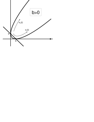
Figure 9: The parabola.

Now we can do the $s$-integration with the aid of an Euler’s change of variables [12] and obtain

$$V^{\prime}=\frac{1}{|c|}\int\limits_{0}^{\infty}\frac{1}{t+t_{0}}\left(f(s_{0},\sigma_{i})+ik(t)g(s_{0},\sigma_{i})\right)\,dt$$ (19)

with

$$f(s_{0},\sigma_{i})=\left\{\begin{array}[]{lll}\frac{2}{\sqrt{-R}}\arctan\left(\frac{s_{0}\pm\sqrt{\sigma_{1}\sigma_{2}}}{\sqrt{-R}}\right)&\mbox{if}\quad\sigma_{1}<-s_{0}<\sigma_{2}&\mbox{(i)}\\ -\frac{1}{\sqrt{R}}\log\left|\frac{s_{0}\pm\sqrt{\sigma_{1}\sigma_{2}}+\sqrt{R}}{s_{0}\pm\sqrt{\sigma_{1}\sigma_{2}}-\sqrt{R}}\right|&\mbox{else}&\mbox{(ii)}\end{array}\right.$$ (20)

and

$$g(s_{0},\sigma_{i})=\left\{\begin{array}[]{lll}\frac{i}{\sqrt{-R}}&\mbox{if}\quad\sigma_{1}<-s_{0}<\sigma_{2}&\mbox{(i)}\\ \frac{1}{\sqrt{R}}&\mbox{else}&\mbox{(ii)}\end{array}\right.$$ (21)

where we note that $s_{0}$ and $\sigma_{i}$ are functions of $t$ and further $R=s_{0}^{2}+s_{0}(\sigma_{1}+\sigma_{2})+\sigma_{1}\sigma_{2}$ and $k=-2,-1,0,1$ or 2, depending on the relative magnitudes of $s_{0}$ and $\sigma_{1/2}$ and the sign of the imaginary part of $s_{0}$. One has to choose $+\sqrt{\sigma_{1}\sigma_{2}}$ in eqs.(20) and (21) if $t>-b/a$, and $-\sqrt{\sigma_{1}\sigma_{2}}$ else. The condition $\sigma_{1}<-s_{0}<\sigma_{2}$ is equivalent to $R<0$.

The $t$-intervals where $k$ is constant, together with the corresponding $k$ values, can be calculated by solving $s_{0}=0$ and $s_{0}=-\sigma_{i}$ for $t$. With another Euler’s change of variables, using eq.(17) and exploiting the relevant properties of the functions $\log(x)$ and $\arctan(x)$, the $t$-integration leads to expressions of the form

$${\mbox{P$\!$.V$\!$.}}\!\int\limits_{x_{1}}^{x_{2}}\frac{1}{x^{2}+px+q}\quad\mbox{from}\;\;g(s_{0},\sigma_{i})\,,$$ (22)

$${\mbox{P$\!$.V$\!$.}}\!\int\limits_{x_{1}}^{x_{2}}\frac{\arctan(rx+s)}{x^{2}+px+q}\quad\mbox{from}\;f(s_{0},\sigma_{i}),\;\mbox{case (i)}$$ (23)

and

$${\mbox{P$\!$.V$\!$.}}\!\int\limits_{x_{1}}^{x_{2}}\frac{\log|x^{2}+rx+s|}{x^{2}+px+q}\quad\mbox{from}\;f(s_{0},\sigma_{i}),\;\mbox{case (ii)}\,,$$ (24)

which can be expressed in terms of logarithms, arcus-tangens, dilogarithms and Clausen’s functions [15], as it was the case for the planar topology. The full result is, as expected, a lengthy expression in terms of these special functions, which we cannot list here. We rather follow the philosophy of [3] and present examples in the next section.

We stress that to obtain stable numerical results in the two dimensional integral over $l_{0}$ and $k_{0}$ it is very important to add all contributions (real and complex) to the same $l_{0}$ and $k_{0}$, because eq.(7) introduces some artificial divergences which cancel in the sum.

As expected, the numerical integrand for the crossed topology is of the same nature as for the planar case, but involves more terms and different cases. This naturally increases the amount of CPU time needed to obtain the requested accuracy: as a thumb rule, we found that the crossed topology demands 5-10 times more time compared to the planar case.

The threshold behaviour can be examined with the four-fold integral representation eq.(13). The crossed vertex function has three two-particle thresholds and six three-particle thresholds. As stated above a possible source for an imaginary part is a negative argument of the square root. A necessary condition for this to happen is $b>0$ for some $l_{0}$, $k_{0}$ inside the integration region. It can be shown that each three-particle threshold corresponds to one of the six $b$ coefficients of the complex triangles [6]. The other $b$ coefficients belonging to the real regions are identical and correspond to the two-particle threshold $q^{2}>(m_{1}+m_{2})^{2}$. The remaining two-particle thresholds $q_{1}^{2}>(m_{3}+m_{5})^{2}$ and $q_{2}^{2}>(m_{4}+m_{6})^{2}$ can be identified with the coefficients $\bar{s}_{01}$ (when $\tilde{a}_{1}=0$) and $\bar{t}_{01}$ respectively which produce an imaginary part when $\bar{s}_{01}$ and $\bar{t}_{01}$ become negative. A possible four-particle threshold $q^{2}>(m_{3}+m_{4}+m_{5}+m_{6})^{2}$ disconnects the graph into three parts and is therefore a combination of the two two-particle thresholds $q_{1}^{2}>(m_{3}+m_{5})^{2}$ and $q_{2}^{2}>(m_{4}+m_{6})^{2}$.

3 Examples

Only few analytical and/or numerical results are known for the crossed vertex function to compare with. Besides the symmetries with respect to internal masses and external momenta, some limiting cases can be checked. In the case of zero momentum transfer the crossed vertex function reduces to the master two-point topology [1, 7] with a squared propagator. fig.10 shows these limits for some arbitrary masses ($m_{1}=2$, $m_{2}=3$, $m_{3}=1$, $m_{4}=1.5$, $m_{5}=0.6$ and $m_{6}=0.2$), $q^{2}=1$ and either $q_{1}\to 0$ or $q_{2}\to 0$. Additionally, for vanishing $q^{2}$ we obtain the vacuum bubble calculated in [16].

Figure 10: Ratio of crossed vertex-function to master two-point function for $q_{1}$ (short dash) and $q_{2}\to 0$ (long dash).

For the case of all internal masses vanishing an analytical formula in known [14]. This limit is approached smoothly in fig.11 for all masses going to zero simultaneously and $e_{1}=4$, $e_{2}=3$ and $q_{z}=1$.

Figure 11: Limit of all masses vanishing.

In the limit of the momenta of the outgoing particles on the light-cone ($q_{1}^{2}=q_{2}^{2}=0$) and all internal masses equal this diagram can be calculated with the small momentum expansion technique [4]. A comparison for real and imaginary part is show in fig.12.

Figure 12: All masses equal, $q_{1}^{2}=q_{2}^{2}=0$, real part (left) and imaginary part (right).

We can obtain this limit easily by transforming our parallel space coordinates to light cone coordinates, which does not interfere with our subsequent steps.

As a last example in fig.13 we show the decay $\rm Z\to t\bar{t}$ with the exchange of two Z bosons. This diagram has been calculated in [5] by a five-dimensional numerical integration over the Feynman parameters.

Figure 13: Decay $\rm Z\to t\bar{t}$, real part.

Conclusions

In this paper, we demonstrated the calculation of the two-loop vertex function for the crossed topology. We outlined how to achieve the reduction to a manageable two-fold integral representation, and verified its correctness by comparison with the literature, wherever data were available. Further, our integral representation was used in [10], with results in perfect agreement with the expectations.

Our results complement the results for the planar topology in [3]. Together, the scalar two-loop three-point function is now available in $D=4$ dimensions for all topologies, all masses, and arbitrary external momenta. Some degenerated topologies were already given in [10], obtained by similar methods. Such degenerated cases typically also appear when one confronts tensor integrals. For the future, we plan to incorporate such cases in the package XLOOPS [6]. Also, code which implements the results presented here will be incorporated there.

To our knowledge, no other method is at this stage able to deliver reliable results for the massive two-loop vertex function in such generality and accuracy.

References

- [1] D. Kreimer. Phys. Lett. B273 (1991) 277.
- [2] D. Kreimer. Phys. Lett. B292 (1992) 341.
- [3] A. Czarnecki, U. Kilian and D. Kreimer, Nucl. Phys.B433 (1995) 259.
- [4] O.V. Tarasov. An algorithm for small momentum expansion of Feynman diagrams, publ. in the proceedings of AIHENP95: New Computing Techniques in Physics Research IV, Eds. B. Denby, D. Perret-Gallix, World Scientific (1995).
- [5] J. Fujimoto, Y. Shimizu, K. Kato and T. Kaneko, Numerical approach to two-loop three point functions with masses, publ. in the proceedings of AIHENP95: New Computing Techniques in Physics Research IV, Eds. B. Denby, D. Perret-Gallix, World Scientific (1995).
-
[6]
L.Brücher, J.Franzkowski,
A.Frink, D.Kreimer, contributed talks given at AIHENP96,
Lausanne, September 1996, to appear.
See also the homepage
http://dipmza.physik.uni-mainz.de/∼Bruecher/xloops.html - [7] S. Bauberger and M. Böhm. Nucl. Phys. B445 (1995) 25.
- [8] J. Fujimoto, Y. Shimizu, K. Kato and Y. Oyanagi, Numerical approach to two-loop integrals, publ. in the proceedings of the workshop on HEP and QFT, Sochi (1992), in Phys.Atom.Nucl.56.
- [9] J. Fleischer and O.V. Tarasov. Z.Phys.C64 (1994) 413.
- [10] A.Frink, B.Kniehl, D.Kreimer, K.Riesselmann. Phys.Rev.D54 (1996) 4548.
- [11] P. Henrici. Applied and computational complex analysis, Vol.I. John Wiley & Sons, New York, 1974.
- [12] G.M. Fichtenholz. Integral and differential calculus, Vol. II. Fizmatgiz, Moscow, 1959.
- [13] N.I. Ussyukina and A.I. Davydychev. Phys. Lett. B298 (1993) 363.
- [14] N.I. Ussyukina and A.I. Davydychev. Phys. Lett. B332 (1994) 159.
- [15] L. Lewin. Polylogarithms and associated functions. North Holland, New York, 1981.
- [16] A.I. Davydychev and J.B. Tausk. Nucl. Phys. B397 (1993) 123.