DTP/96/88

hep-ph/9610284

October 1996

Supersymmetric QCD corrections to the
$W$-boson width

A. B. Lahanas ^a   and   V. C. Spanos ^b
a University of Athens, Physics Department, Nuclear and Particle Physics Section,
GR–15771 Athens, Greece

^b University of Durham, Department of Physics,
Durham DH1 3LE, England

We calculate the one-loop supersymmetric QCD corrections to the width of the $W$-boson. We find that these are of order $\sim{{\alpha_{s}}\over{\pi}}{1\over 20}{{M^{2}_{W}}\over{M_{S}^{2}}}\Gamma_{u{\bar{d}}}$, where $M_{S}$ is the supersymmetry breaking scale and $\Gamma_{u{\bar{d}}}$ the tree level hadronic width for $W^{+}\rightarrow u{\bar{d}}$. Due to the appearance of the suppression factor $\sim{1\over 20}$ these are at least two orders of magnitude smaller than the standard QCD corrections $\sim{{\alpha_{s}}\over{\pi}}\Gamma_{u{\bar{d}}}$ and hence of the order of the two-loop electroweak effects. Therefore supersymmetric QCD corrections will only be of relevance once experiments reach that level of accuracy.

 
E-mail:   ^a alahanas@atlas.uoa.gr, ^b V.C.Spanos@durham.ac.uk

The second phase of the LEP (LEP2) collider has already started, and the first $e^{+}e^{-}\rightarrow W^{+}W^{-}$ events have been collected. Studying for the very first time directly this process, one will have the opportunity to test the non-abelian character of the Standard Model (SM), through the precise measurements of the trilinear gauge boson couplings. In addition, it will be possible to measure precisely the mass and width of the $W$-boson [1]. Specifically the measurement of the $W$-width is of special interest, as it is used as an input parameter in many other processes. (It is understood that all the $W$ production events are detected through the hadronic and/or (semi)leptonic decays of the $W$-boson.) So it is very essential, both for theoretical and experimental reasons, to know as precise as possible the theoretical prediction for this parameter.

The one-loop corrections to the $W$-width in the context of the Standard Model (SM) are already known [2, 3], and there has been also a calculation in the context of a two Higgs doublet model [4].

The possible existence of new physics of characteristic scale $M_{new}$ may affect the theoretical predictions for the $W$-boson decay width. The magnitude of these effects is not a priori known without knowledge of the underlying theory and thus manifestation of new physics from a direct measurement of the $W$-boson width is not possible. The corrections to the $W$-boson observables which are induced by new physics are expected to be small, possibly smaller than the experimental precision of LEP2 which will be in the percent region. With increasing experimental accuracy in the future, the $W$-boson observables may provide a laboratory for testing new physics and Supersymmetry is a prominent candidate.

It is known that strong interaction effects yield the largest contribution, ${\cal O}(4\%)$, to the $W$-width at the one-loop order. With the SM being promoted to a supersymmetric theory, the QCD sector is also supersymmetrized (SQCD) and new species which interact strongly affect the QCD predictions. Therefore it seems natural to calculate the SQCD corrections to the hadronic width of the $W$. The size of these corrections depends on the supersymmetry breaking scale $M_{S}$ and is obviously negligible as $M_{S}$ becomes large. However the existing experimental lower bounds on sparticle masses does not exclude values of $M_{S}$ in the vicinity of the electroweak scale $M_{S}\simeq{\cal O}$(few $M_{W}$), in which case these effects may not be suppressed.

In this Letter we undertake this problem and calculate the supersymmetric QCD corrections to the $W$-boson width. We perform our calculations using the on-shell renormalization scheme [6, 7] which has been extensively used in the SM calculations (see for instance Ref. [8, 9]). In order to study the SQCD corrections to the $W$-boson hadronic width we need to calculate the corrections to $Wu\bar{d}$ vertex as well as the wave function renormalizations to the external fermion propagators (see Fig. 1(a) and (b) respectively). In order to simplify our discussion we shall neglect mixings of the up ${\tilde{u}}_{L},{\tilde{u}}_{L}^{c}$ and down ${\tilde{d}}_{L},{\tilde{d}}_{L}^{c}$ left handed squarks of the first two generations since these mixings are proportional to the corresponding fermion masses and hence small. Therefore the above squark states are mass eigenstates in this approximation.

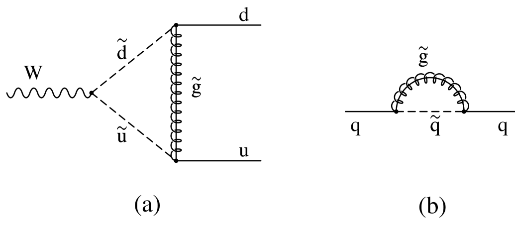
Figure 1: Graphs which contribute to the one-loop supersymmetric QCD corrections to the $W$-width. There are corrections to the $Wu\bar{d}$ vertex (a) and corrections to the external quark propagators (b).

By using the well known Passarino–Veltman functions [7, 10] $B_{0},B_{1},B_{1}^{\prime},C_{0},C_{1},C_{ij}$ etc., through which the two and three point functions are usually expressed, we find for the $Wu\bar{d}$ vertex correction of Fig. 1(a)

$${\cal A}_{1}\,=\,i({{\alpha_{s}}\over{2\pi}}){g\over\sqrt{2}}\,c_{F}\,[(2C_{24})\,M_{0}+2M_{u}(C_{21}+C_{11}-C_{12}-C_{23})\,M_{2}$$

$$\hskip 99.58464pt+\,2M_{d}(C_{23}+C_{12})\,M_{3}\,].$$ (1)

In the equation above the four basic amplitudes $M_{0,1,2,3}$ are as in Ref. [3], $g$ is the weak coupling constant and $\alpha_{s}={g^{2}_{s}\over(4\pi)}$, where $g_{s}$ is the strong coupling constant. $M_{u,d}$ are the masses of the $u,d$ external quarks and the factor $c_{F}=4/3$ is the value of the quadratic Casimir operator of the fundamental representation of the SU(3) symmetry group. The arguments of the $C_{ij}$ functions appearing above are defined as follows:

$$C_{ij}\,=\,{C_{ij}}(p_{1},-p_{1}-p_{2},M^{2}_{\tilde{g}},m^{2}_{{\tilde{u}}_{L}},m^{2}_{{\tilde{d}}_{L}}).$$

In this expression $p_{1}(-p_{2})$ is the momentum carried by the outgoing (incoming) $u(d)$ quark. The ultraviolet infinity of the vertex correction is contained within the factor $C_{24}$ of the amplitude $M_{0}$. This infinity is canceled by the vertex counterterm in the Lagrangian [9],

$${\Delta L}_{CT}\,=\,(\delta Z_{L}+\delta Z_{1}^{W}-\delta Z_{2}^{W})\,{g\over\sqrt{2}}W_{\mu}^{+}{\bar{u}}_{L}{\gamma^{\mu}}{d_{L}},$$ (2)

$\delta Z_{L}\equiv Z_{L}-1$, where $Z_{L}$ is the wave function renormalization constant of the left handed doublet $(u_{L},d_{L})$. There are no strong interaction contributions to the difference $\delta Z_{1}^{W}-\delta Z_{2}^{W}$ so that only $\delta Z_{L}$ needs be considered. For the down quark the on-shell renormalization condition is

$${S_{down}}(P)\,\,{\stackrel{{\scriptstyle{\mathchoice{\ooalign{$\hfil\displaystyle\mkern 0.0mu/\hfil$\crcr$\displaystyle P$}}{\ooalign{$\hfil\textstyle\mkern 0.0mu/\hfil$\crcr$\textstyle P$}}{\ooalign{$\hfil\scriptstyle\mkern 0.0mu/\hfil$\crcr$\scriptstyle P$}}{\ooalign{$\hfil\scriptscriptstyle\mkern 0.0mu/\hfil$\crcr$\scriptscriptstyle P$}}}\rightarrow M_{d}}}{{\longrightarrow}}}\,({\mathchoice{\ooalign{$\hfil\displaystyle\mkern 0.0mu/\hfil$\crcr$\displaystyle P$}}{\ooalign{$\hfil\textstyle\mkern 0.0mu/\hfil$\crcr$\textstyle P$}}{\ooalign{$\hfil\scriptstyle\mkern 0.0mu/\hfil$\crcr$\scriptstyle P$}}{\ooalign{$\hfil\scriptscriptstyle\mkern 0.0mu/\hfil$\crcr$\scriptscriptstyle P$}}}-M_{d})^{-1},$$ (19)

where ${S_{down}}(P)$ denotes the down quark propagator. This fixes the wave function renormalization constant of both left and right handed components of the down quark. By a straightforward calculation of the graph shown in Fig. 1(b), and using Eq. (19), we find for $\delta Z_{L}$, which is needed for our calculation,

$$\delta Z_{L}=({{\alpha_{s}}\over{2\pi}})\,c_{F}\,[{B_{1}}(M^{2}_{d},M^{2}_{\tilde{g}},m^{2}_{{\tilde{d}}_{L}})+M^{2}_{d}\,({{B_{1}}^{\prime}}(M^{2}_{d},M^{2}_{\tilde{g}},m^{2}_{{\tilde{d}}_{L}})+{{B_{1}}^{\prime}}(M^{2}_{d},M^{2}_{\tilde{g}},m^{2}_{{\tilde{d}}_{L}^{c}}))]$$

$$\equiv{{\Pi}_{d}}(M^{2}_{d}).$$ (20)

Therefore the SQCD contribution of the vertex counterterm to the $W^{+}\rightarrow u\bar{d}$ amplitude is

$${{\cal A}_{1}}^{\prime}\,=\,i{g\over\sqrt{2}}M_{0}\,(\delta Z_{L}),$$ (21)

with $\delta Z_{L}$ as given above.

Having fixed the the renormalization constant $Z_{L}$ it is convenient to choose the renormalization constant of the right handed up quark is such a way that the residues for the left and right handed propagators are equal (see for instance Ref. [3, 8, 9]). Thus we have for the up quark propagator

$${S_{up}}(P)\,\,{\stackrel{{\scriptstyle{\mathchoice{\ooalign{$\hfil\displaystyle\mkern 0.0mu/\hfil$\crcr$\displaystyle P$}}{\ooalign{$\hfil\textstyle\mkern 0.0mu/\hfil$\crcr$\textstyle P$}}{\ooalign{$\hfil\scriptstyle\mkern 0.0mu/\hfil$\crcr$\scriptstyle P$}}{\ooalign{$\hfil\scriptscriptstyle\mkern 0.0mu/\hfil$\crcr$\scriptscriptstyle P$}}}\rightarrow M_{u}}}{{\longrightarrow}}}\,{z_{u}}\,({\mathchoice{\ooalign{$\hfil\displaystyle\mkern 0.0mu/\hfil$\crcr$\displaystyle P$}}{\ooalign{$\hfil\textstyle\mkern 0.0mu/\hfil$\crcr$\textstyle P$}}{\ooalign{$\hfil\scriptstyle\mkern 0.0mu/\hfil$\crcr$\scriptstyle P$}}{\ooalign{$\hfil\scriptscriptstyle\mkern 0.0mu/\hfil$\crcr$\scriptscriptstyle P$}}}-M_{d})^{-1}.$$ (38)

Note that since left handed up ($I_{3}=1/2$) and down ($I_{3}=-1/2$) components belong to the same multiplet and $Z_{L}$ has already been fixed by Eq. (19) we cannot have $z_{u}=1$. The residue $z_{u}$ is finite and is given by

$$z_{u}\,\equiv\,1+{\delta z_{u}}\,=\,1\,+\,({{\alpha_{s}}\over{2\pi}})\,c_{F}\,({{\Pi}_{u}}(M^{2}_{u})-{{\Pi}_{d}}(M^{2}_{d})).$$ (39)

The ${{\Pi}_{u}}(M^{2}_{u})$ appearing above is in form identical to ${{\Pi}_{d}}(M^{2}_{d})$ defined in Eq. (20) with the replacements $M_{d},m_{{\tilde{d}}_{L}},m_{{\tilde{d}}_{L}^{c}}\rightarrow M_{u},m_{{\tilde{u}}_{L}},m_{{\tilde{u}}_{L}^{c}}$.

Since ${\delta z_{u}}\neq 1$ we have an additional contribution to the amplitude which stems from the wave function renormalization of the external up quark line; at the one-loop level this is given by

$${{\cal A}_{2}} = i\;{g\over\sqrt{2}}M_{0}\;({{\delta z_{u}}\over 2})$$ (40)

$$= i\;c_{F}\,{{g{\alpha_{s}}}\over{4\pi\sqrt{2}}}({{\Pi}_{u}}(M^{2}_{u})-{{\Pi}_{d}}(M^{2}_{d}))\,M_{0}.$$

This completes our calculation of the SQCD corrections to the amplitude for $W^{+}\rightarrow u{\bar{d}}$.

We now proceed to discussing the corrections to the hadronic width of the $W$-boson. The one-loop hadronic width $\Gamma^{(1)}$ can be written as

$$\Gamma^{(1)}\,=\,{\Gamma_{u{\bar{d}}}^{(0)}}\,(1\,+\,{\delta}),$$ (41)

where ${\Gamma_{u{\bar{d}}}^{(0)}}$ is the tree level hadronic width for one family. In the limit of vanishing quark masses this is given by ${\Gamma_{u\bar{d}}^{(0)}}\,=\,{{\alpha}_{w}}M_{W}/4$. The SQCD corrections to ${\delta}$ can be found from the amplitudes ${\cal A}_{1},{{\cal A}_{1}}^{\prime},{\cal A}_{2}$ we have just calculated. It is found that

$$\delta^{SQCD}\,=\,{{\alpha_{s}}\over{\pi}}\,c_{F}\,[\,2C_{24}+B_{1}+{{\Pi_{u}-\Pi_{d}}\over 2}\,]+...$$ (42)

In order to avoid confusion we should say that $\delta^{SQCD}$ accounts for only the supersymmetric corrections, that is those due to the exchange of gluinos and squarks. The functions $C_{24},B_{1},\Pi_{u,d}$ are as they appear in the definitions of the amplitudes ${\cal A}_{1},{\cal A}_{1}^{\prime},{\cal A}_{2}$, while the ellipses denote terms proportional to the external quark masses. In the limit of vanishing quark masses, $\delta^{SQCD}$ can be cast in the following integral form

$${\delta}^{SQCD}\, = \,{{2\alpha_{s}}\over{3\pi}}{\int_{0}^{1}xdx\int_{0}^{1}dy}$$ (43)

$$\times\,{\ln\,\{{{(xm^{2}_{{\tilde{u}}_{L}}+(1-x)M^{2}_{{\tilde{g}}})\,(xm^{2}_{{\tilde{d}}_{L}}+(1-x)M^{2}_{{\tilde{g}}})}\over{(M^{2}_{W}x^{2}y(y-1)+(m^{2}_{{\tilde{d}}_{L}}-m^{2}_{{\tilde{u}}_{L}})xy+(m^{2}_{{\tilde{u}}_{L}}-M^{2}_{{\tilde{g}}})x+M^{2}_{{\tilde{g}}})^{2}}}}\}.$$

¿From the form above we can easily get first estimates of the magnitude of the SQCD corrections as will be seen in the sequel.

Figure 2: The function $F(a)$ and its derivative as described in the text.

In order to simplify the discussion let us assume that $m_{{\tilde{u}}_{L}}\approx m_{{\tilde{d}}_{L}}\approx M_{{\tilde{g}}}=M_{S}$, where $M_{S}$ sets the order of the supersymmetry breaking scale. In this case the expression above for ${\delta}^{SQCD}$ is simplified, to become

$${\delta}^{SQCD}\,=\,{{4\alpha_{s}}\over{3\pi}}{\int_{0}^{1}xdx\int_{0}^{1}dy}\ln\,\{{{M_{S}^{2}}\over{M^{2}_{W}x^{2}y(y-1)+M_{S}^{2}}}\}$$

$$\equiv{{4\alpha_{s}}\over{3\pi}}F(M^{2}_{W}/M_{S}^{2}).$$ (44)

Since $M_{S}>M_{W}$ the function $F(M^{2}_{W}/M_{S}^{2})$ can be expanded in powers of $a\equiv M^{2}_{W}/M_{S}^{2}$. The result of such an expansion is

$$F(a)={a\over 24}+{{a^{2}}\over 360}+{{a^{3}}\over 3360}+...$$ (45)

Keeping the first term of the expansion results in

$${\delta}^{SQCD}\, = \,{{\alpha_{s}}\over{\pi}}{1\over 18}{{M^{2}_{W}}\over{M_{S}^{2}}}.$$ (46)

${\delta}^{SQCD}$ is very well approximated by keeping only the leading term in the expansion of $F$ as can be seen from Fig. 2 where both the function and its derivative are plotted. In fact the function $F(a)$ is almost linear in the interval $0<a<1$ with almost constant derivative, justifying the linear approximation to $F$ which led to the result above. Note the appearance of an extra suppression factor $1/18$ in addition to the expected ${{M^{2}_{W}}\over{M_{S}^{2}}}$ factor due to the decoupling of sparticles as we pass below the scale $M_{S}$. This situation persists also in other cases as for instance when the gluino is lighter than the squarks, i.e $M_{\tilde{g}}\ll m_{{\tilde{u}}_{L},{\tilde{d}}_{L}}$. In that case employing the fact that $\Delta m^{2}\equiv m^{2}_{{\tilde{d}}_{L}}-m^{2}_{{\tilde{u}}_{L}}\ll m^{2}_{{{\tilde{u}}_{L}},{{\tilde{d}}_{L}}}\equiv M_{S}^{2}$, since the difference of the masses squared of the ${\tilde{u}}_{L},{\tilde{d}}_{L}$ squarks is of the order of the electroweak scale, we get in an analogous way exactly the same result with the suppression factor $1/18$ being replaced by $2/27$. Our complete numerical analysis uses the full expression for $\delta^{SQCD}$ and has actually covered the whole parameter space of the MSSM assuming universal boundary conditions for the squark masses at the unification point where the couplings merge. In all cases the SQCD corrections turned out to be of the order ${\cal O}(5\%){{\alpha_{s}}\over{\pi}}{{M^{2}_{W}}\over{M_{S}^{2}}}$ or less, instead of the expected ${{\alpha_{s}}\over{\pi}}{{M^{2}_{W}}\over{M_{S}^{2}}}$ behaviour. If we compare this with ${{\alpha_{s}}\over{\pi}}$, which is the contribution of gluons to $\delta$, we see that the appearance of gluinos and squarks has a negligible effect $\leq{\cal O}(10^{-2}){{\alpha_{s}}\over{\pi}}$ on the hadronic width of the $W$-boson. Actually in the constrained MSSM with radiative symmetry breaking, these corrections turn out to be even smaller ${\cal O}(10^{-3}-10^{-4}){{\alpha_{s}}\over{\pi}}$. Therefore supersymmetric QCD corrections to the $W$-boson width are at best of the order of the two-loop electroweak corrections and not of relevance to current experiments.

Acknowledgements
We want to thank James Stirling for a careful reading of this manuscript. This work was supported by the EU Human Capital and Mobility Programme, CHRX–CT93–0319.

References

• [1] โ€˜Determination of the Mass of the $W$ Bosonโ€™, Z.ย Kunszt and W.J.ย Stirling et al., in Physics at LEP2, eds. G.ย Altarelli, T.ย Sjรถstrand and F.ย Zwirner, CERN Report 96-01 (1996), vol.1, p.ย 141;
โ€˜WW cross-sections and distributionsโ€™, W. Beenakker and F.A. Berends et al., in Physics at LEP2, eds. G.ย Altarelli, T.ย Sjรถstrand and F.ย Zwirner, CERN Report 96-01 (1996), vol. 1, p.ย 81.
• [2] T.H.ย Chang, K.J.F.ย Gaemers and W.L.ย vanย Neerven, Nucl. Phys. B202 (1982) 407;
K.ย Inoue, A.ย Kakuto, H.ย Komatsu and S.ย Takeshita, Prog. Theor. Phys. 64 (1980) 1008;
D.ย Bardin, S.ย Riemann and T.ย Riemann, Z. Phys. C 32 (1986) 121;
J.W.ย Jun and C.ย Jue, Mod. Phys. Lett. A6 (1991) 2767.
• [3] A.ย Denner and T.ย Sack, Z. Phys. C 46 (1990) 653.
• [4] D.-S.ย Shin, Nucl. Phys. B449 (1995) 69.
• [5] J.ย Rosner, M.ย Worah and T. Takeuchi, Phys. Rev. D49 (1994) 1363.
• [6] D.A.ย Ross and J.C.ย Taylor, Nucl. Phys. B51 (1973) 125.
• [7] G.ย Passarino and M.ย Veltman, Nucl. Phys. B160 (1979) 151.
• [8] M.ย Bรถhm, H.ย Spiesberger and W.ย Hollik, Fortschr. Phys. 34 (1986) 687.
• [9] โ€œRenormalization of the Standard Modelโ€, W.ย Hollik, appears in Precision tests of the Standard Model, Advanced series on directions in high-energy physics, ed. Paul Langacker, World Scientific, 1993.
• [10] G.ย โ€™t Hooft and M.ย Veltman, Nucl. Phys. B153 (1979) 369.